Finding Banded Patterns in Data: The Banded Pattern Mining Algorithm

Finding Banded Patterns in Data: The Banded

Pattern Mining Algorithm

Fatimah B. Abdullahi, Frans Coenen, and Russell Martin

The Department of Computer Science, The University of Liverpool, Ashton Street, Liverpool, L69 3BX, United Kingdom

email:{f.b.abdullahi,coenen,russell.martin}@liverpool.ac.uk

Abstract. The concept of Banded pattern mining is concerned with the identification of “bandings” within zero-one data. A zero-one data set is said to be fully banded if all the “ones” can be arranged along the leading diagonal. The discovery of a banded pattern is of interest in its own right, at least in a data analysis context, because it tells us something about the data. Banding has also been shown to enhances the efficiency of matrix manipulation algorithms. In this paper the exact N dimensional Banded Pattern Mining (BPM) algorithm is presented together with a full evaluation of its operation. To illustrate the utility of the banded pattern concept a case study using the Great Britain (GB) Cattle movement database is also presented.

Keywords: Banded Patterns, Zero-One data, Banded Pattern Mining

1

Introduction

Banded pattern mining is concerned with the identification of “bandings” within zero-one data [7, 10, 8, 9]. The idea is, given a zero-one data set, to rearrange the elements in each dimensions so that a banding is revealed. A zero-one data set is said to be fully banded if all the “ones” can be arranged along the leading diago-nal. Typically a perfect banding cannot be discovered, however it is still possible to rearrange the data to reveal a nearest possible banding. The discovery of a banded pattern is of interest in its own right, at least in a data mining context, because it tells us something about the data. Banding has also been shown to improve the operation of variousndimensional matrix manipulation algorithms in that only the portion of the matrix located near the leading diagonal needs to be considered.

The rest of this paper is organised as follows. Section 2 presents some relevant previous work, concentrating on the MBA and BC algorithms. Section 3 presents some formalism concerning the banded pattern problem, while Section 4 presents the proposed BPM algorithm. To aid in the understanding of the BPM algorithm Section 5 presents a worked example. A full evaluation, using both artificial and real data sets, is presented in Section 6. Some conclusion are given in Section 7.

2

Previous Work

The concept of banded matrices, from the data analysis perspective, occurs in many applications domains; examples can be found in paleontology [2], Network data analysis [3] and linguistics [8]. More recent work can be found in [7] and [10]. The current state of the art algorithm, the Minimum Banded Augmen-tation (MBA) proposed by [8], focuses on minimizing the distance of non-zero entries from the main diagonal of a matrix by reordering the original matrix. The MBA algorithm operates by “flipping” zero entries (0s) to one entries (1s) and vice versa to identify a banding. Gemma et al. fixed the column permu-tations of the data matrix before executing their algorithm [7]. Here the basic idea is to solve optimally the consecutive one property on the permuted ma-trix M and then resolve “Sperner conflicts” to eliminate all the overlapping row intervals between each row of the permuted matrix, by going through all the extra rows and making them consecutive. While it can be argued that the fixed column permutation assumption is not a very realistic assumption with respect to many real world situations, heuristical methods were proposed in [7] to determine a suitable fixed column permutation. The MBA algorithm use the Accuracy (Acc) measure to evaluate the performance of the banding produced. Another frequently referenced banding strategy is the Barycentric (BC) algo-rithm that transposes a matrix. It was originally designed for graph drawing, but more recently used to reorder binary matrices [9]. The BC algorithm uses the Mean Row Moment (M RM) measure to evaluate the performance of the banding produced. The distinction between these previous algorithms and that presented in this paper is that the previous algorithms were all directed at 2D data, while the proposed algorithm operates in ND. The above MBA and BC algorithms are the two examplar banding algorithms with which the operation of the proposed BPM algorithm was compared and evaluated as discussed later in this paper. Note that Bandwidth minimization of binary matrices is known to be NP-Complete [5].

3

Formalism

Note that dimensions are not necessarily all of the same size. However there is a correspondence between eachdimiandposipairing (|dimi| ≡ |posi|). Initially the content of each set dimi will be the same as the content of each set posi, however it is the elements in each setposi inP OSthat we wish to rearrange so as to identify a banding.

Each “cell” in thendimensional data space is thus identifiable by a coordi-nate tuple of lengthn, hc1, c2. . . cni; wherec1 ∈dimi, c2 ∈dim2 and so on. If

n= 2 we might think of these as x-y coordinates, and ifn= 3 we might think of these as x-y-z coordinates. Each cell contains either a 1 or 0. For illustrative pur-poses, in the remainder of this paper, we say that a cell with a 1 value contains a “dot”, and a cell with a 0 is empty.

The data setsD={d1, d2, . . .}we are interested in thus comprise a sequence

ofk coordinate tuples each of size nand each reprsenting a “dot”. Note that a specific coordinate tuple can appear only once inD. Each tuple thus describes the location of a dot in the data space. It is these dots that we wish to arrange in such a manner that they are as close to the leading diagonal as possible by rearranging the position of the indexes (coordinates).

4

The Banded Pattern Mining Algorithm

A high level view of the proposed Banded Pattern Mining (BPM) algorithm is presented in Algorithm 1. The algorithm describes an iterative approach whereby the elements in each dimension are repeatedly rearranged until a best banding score is arrived at or until some maximum number of iterations is reached. The algorithm is founded on ideas presented in [1] where an approximate BPM algorithm (BPMA) was presented. Comparison are made later in Section 6 using both the proposed exact BPM algorithm and the previous BPMAalgorithm. The inputs to the algorithm are: (i) a zero-one data setDwhich is to be banded, (ii) a desired maximum number of iterationsmaxand (iii) the set of dimensionsDIM describing then dimensional data space to whichD subscribes. The Output is a rearranged data setD0.

On each iteration each dimensiondimiinDIMis considered in turn. For each element j in dimi a normalised banding score bsij is calculated (line 12) using equation 2 (the derivation of the equation is described in more detail below). The elements in dimension dimi are then rearranged (line 14) in descending order according to the banding scores calculated earlier. If two or more elements have the same banding score (an unlikely event given a large data set) then the number of dots featured in each element is taken into consideration together with the relative position of the new location with respect to the centroid of the data space (essentially we wish to place elements with larger numbers of dots closer to the centroid of the current data sub-space than elements with smaller numbers of dots). The rearranging of elements in dimensions is repeated for each dimension in turn.

derived earlier (Equation 2). If the newly calculated banding score is equal or less (worse) than the previously calculated score we break (line18), otherwise we continue onto the next iteration. On completion (line 25) we derive the new dataset D0 using the positions of the indexes contained inDIM. The situation where a worsegbs than that obtained on the previous iteration may be arrived at is where we have a “poling” effect where we are rearranging that data one way, and then another way, without improving the banding.

Algorithm 1The BPM Algorithm 1: Input

2: D= Binary valued input data set

3: max= The maximum number of iterations 4: Output

5: D0= Data setDrearranged so as to display as near a banding as possible 6: gbs= 0 (The global banding score so far)

7: counter= 0

8: whilecounter < maxdo 9: for alldimi∈DIM do 10: forj= 1 toj=|dimi|do

11: bsij= Banding score for elementjin|dimi|calcuated using

12: Equation 2

13: end for

14: dim0i= The setdimirearranged according to the calculatedbs 15: (in descending order)

16: end for

17: gbs0= Global banding score for current configuration described by 18: DIM0={dim01, dim

0

2, . . . , dim 0

n}calculated using Equation 3 19: if gbs0≤gbsthen

20: break

21: else 22: gbs=gbs0 23: DIM=DIM0 24: end if

25: counter=counter+ 1 26: end while

27: D0= Input datasetD rearranged according to index positions inP OS

The banding scorebsij for a particular elementj in dimensiondimiis deter-mined according to the location of the subset of dotsS inDwhosecicoordinate is equal toj(recall that each dot inDis define by a coordinate tuple of the form hc1, c2. . . cni). For each dot in S we calculate the distance to the origin of the data sub-space that does not include dimi. We exclude the current dimension because this is the dimension we want to rearrange. Thus a banding scorebs is calculated as follows:

bs= i=|S|

X

i=1

However, to allow for comparison ofbswe need to normalise the score. Given a dot that is at the origin of the sub-space of interest the normalisedbsshould be 0. Given a dot that is as far away from the the origin of the sub-space of interest as is geometrically possible the normalisedbsshould be 1. Thus to normalisebs we need to divide by the sum of the set of |S|maximum distances that can be attained in the given sub space:

bs=

Pi=|S|

i=1 distT oOrigin(doti)

Pi=|M|

i=1 maxi

(2)

whereM is a set of maximum distances corresponding to the number of dots in S. Note that the content ofM will vary according to the nature of the setDIM for a given data set D. Given that we can identify the coordinate value that features most frequently in the coordinate tuples in D we know the maximum required size ofmax. Given our knowledge ofDIMwe can therefore calculate the values to be included in M at the start of the process (not shown in Algorithm 1) and thus we can calculate these values in advance and store them in a table to be used as necessary. In the evaluation section presented later in this paper a comparison is presented between using a pre calculated BMP “M-table” and calculating maximum distances as required (not using a BPM“M-table”). Using an BPMM-table means that values are only calculated once, although it may be the case that some values are calculated that are never used.

The global banding score,gbsfor a configuration is then given by:

gbs=

Pi=|DIM|

i=1

Pj=|dimi| j=1 bsij

Pk=|DIM|

k=1 |dimk|

(3)

the sum of all the identified banding scores for each element in each dimension. Thus if every element within a given data space is filled with a dot the global banding score will be 1. Distances can be calculated in a variety of ways. Two obvious mechanisms are Manhattan distance and Euclidean distance (both are considered in the evaluation presented later in this paper).

5

Worked Example

The operation of the BPM algorithm can best be illustrated using a worked example. Consider the 2 dimensional 4×4 configuration given in Figure 1(a) (the origin is in the top left hand corner). It has dimensionsDim={x, y}, and:

D={h0,1i,h0,2i,h0,3i,h1,0i,h1,1i,h2,0i,h2,1i,h2,3i,h3,2i,h3,3i}.

(a) Raw Data (b) After rearrangement ofdim1

(c) After rearrangement ofdim2

Fig. 1.Example of operation of BPM algorithm

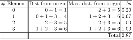
# Element Dist from origin Max. dist. from origin bs 0 1 + 2 + 3 = 6 1 + 2 + 3 = 6 1.00

1 0 + 1 = 1 2 + 3 = 5 0.20

2 0 + 1 + 3 = 4 1 + 2 + 3 = 6 0.67

3 2 + 3 = 5 2 + 3 = 5 1.00

Total 2.87

Table 1.Calculation of banding scores for dimensionx

with the largest number of dots associated with it is nearest to the centre of the data space. The result is as shown in Figure 1(b).

Considering dimensionynext, we calculate banding scores as shown in Table 2. This produces the banding scores 0.20, 0.67, 1.00 and 1.00. The elements iny are more or less already in ascending order ofbs. We only need to swap the last two elements so that the element with the greater number of dots is nearer the centre of the data space. The result is as shown in Figure 1(c).

# Element Dist from origin Max. dist. from origin bs

0 0 + 1 = 1 2 + 3 = 5 0.20

1 0 + 1 + 3 = 4 1 + 2 + 3 = 6 0.67

2 2 + 3 = 5 2 + 3 = 5 1.00

3 1 + 2 + 3 = 6 1 + 2 + 3 = 6 1.00 Total 2.87

Table 2.Calculation of banding scores for dimension y

The global banding score is then the sum of the individual banding scores divided by the total number of elements in the configuration:

gbs=2.87+2₈ .87 = 5.₈73 = 0.72

The process is repeated on the next iteration (not shown here) and the same gbs value produced because we already have a best banding. The rearranged data set D0 arrived at is:

D0 ={h0,0i,h0,1i,h1,0i,h1,1i,h1,2i,h2,1i,h2,2i,h2,3i,h3,2i,h3,3i}.

6

Evaluation

– To determine the effect of data set size and density on the BPM algorithm using artificial data.

– To compare the operation of the BPM algorithm with existing algorithms (MBA and BC) using real data sets.

– To consider the application of the BPM algorithms with respect to a large scale application (the GB cattle movement database).

Each is discussed in further detail in the following three sub-sections.

6.1 Effect of Data Set Size

To determine the efficiency of the proposed BPM algorithm in comparison with the MBA and BC all three algorithms were run using artificial data sets of varying size generated using the LUCS-KDD data generator [6]1_{. Using this}

generator ten data sets measuring 100×100, 141×141, 173×173, 200×200, 224×224, 245×245, 265×265, 283×283, 300×300 and 316×316 were generated, corresponding to numbers of elements approximately increasing from 10,000 to 100,000 in steps of 10,000. A density of 10% was used (in other words 10% of the cells in each row contained a dot). A further five 100×100 data sets were generated using densities from 10% to 50% increasing in steps of 10.

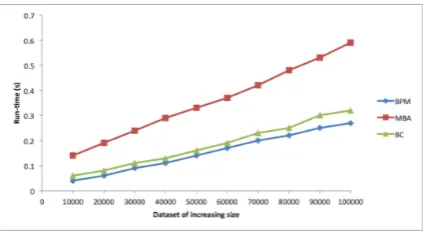
The recorded runtime results obtained by applying the proposed BPM al-gorithm and the MBA and BC alal-gorithms to data sets of increasing size are presented in graph form in Figure 2. From the graph it can be seen that there is a clear correlation between the dataset and the run-time, as the dataset size increases the processing time also increases (this is to be expected).

Fig. 2.Recorded run time (sec.) when the BPM, MBA and BC algorithms are applied to data sets of increasing size (10,000 to 100,000 elements in steps of 10,000)

The recorded runtime results obtained by applying the proposed BPM algo-rithm and the MBA and BC algoalgo-rithms to data sets of increasing density are presented in Figure 3. From the graph it can be seen that there is a correla-tion between the density of the datasets and the run-time as the density of the datasets increases the processing time also increases.

1 _{Available athttp://cgi.csc.liv.ac.uk/frans/KDD/Software/LUCS-KDD-DataGen/}

Fig. 3.Recorded run time (sec.) when the BPM, MBA and BC algorithms are applied to data sets of increasing density (10% to 50% elements in steps of 10)

6.2 Comparison with BPM, MBA and BC

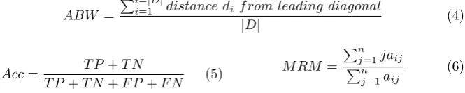
To compare the nature of the bandings produced using BPM, MBA and BC the average width of the banding produced was used as an independent measure (as oppose to global banding score gbs, accuracy Acc and Mean Row Moment M RM). Average Banding Width (ABW) was calculated as shown in Equation 4. Similarly, Acc and Mean Row Moment (M RM) are calculated as shown in Equations 5 and 6:

ABW =

Pi=|D|

i=1 distance di f rom leading diagonal

|D| (4)

Acc= T P +T N

T P +T N+F P+F N (5)

M RM =

Pn

j=1jaij Pn

j=1aij

(6)

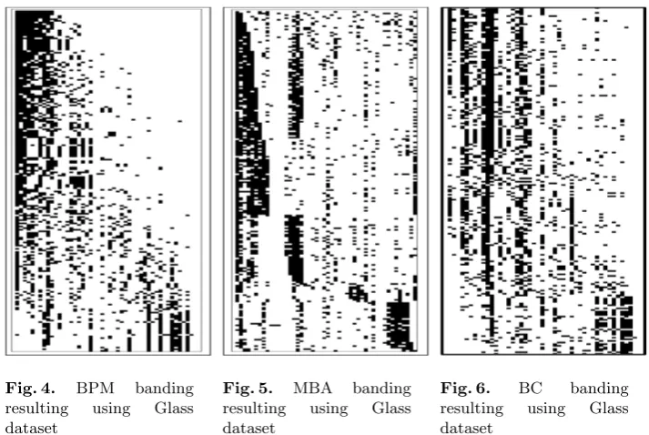
BPM, MBA and BC algorithms respectively. The Figures shows that banding can be identified in all cases. However, considering the banding produced when the MBA algorithm was applied to the glass data sets (Figure 5) the banding result contains dots (“1s”) at top-right and bottom-left corners while the BPM algorithm does not. Similarly, when the BC algorithm was applied to the glass data set (Figure 6) the banding result is less dense than in the case of the proposed BPM algorithm (which features a smaller bandwidth).

Table 3.ABW andgbsresults presented using:BP M,M BAandBCalgorithms

Dataset (column BPM MBA BC BPM MBA BC ×rows) ABW ABW ABW gbs gbs gbs Auto 2050.61250.8182 0.78020.76040.6545 0.6109 Breast 6990.98520.9982 0.99570.88900.7281 0.7423 Car 17280.99160.9983 0.99730.80530.7783 0.7697 Congress 4350.95880.9918 0.98810.88070.8086 0.8018 Cylband 5400.89130.9659 0.94960.84050.7854 0.7417 Dematology 3660.92050.9729 0.97090.81890.7742 0.7553 Ecoli 3360.91490.9908 0.97170.77670.7544 0.7697 Flare 13890.97940.9981 0.99240.80140.7379 0.7807 Glass 2140.83920.9468 0.93910.77440.7503 0.6963 Ionosphere 3510.71520.8295 0.86960.79060.7393 0.6882

Table 4.Acc(%) andM RMresults presented using:BP M,M BAandBCalgorithms

Dataset (column BPM MBA BC BPM MBA BC

×rows ) Acc Acc Acc M RM M RM M RM Auto 205 71.4773.37 73.35 135.64 129.78 130.81 Breast 69952.62 51.25 51.25 437.72 358.75 379.13 Car 1728 61.9762.01 61.13 1168.23 1146.581171.21 Congress 435 55.5255.68 56.34 352.21 348.66 322.72 Cylband 540 62.8663.42 63.32 352.21 348.66 322.72 Dematology 36665.70 65.05 61.79 242.99 238.17 245.77 Ecoli 33661.94 60.36 60.32 254.70 239.50 249.17 Flare 138963.91 63.27 63.211051.571031.53 1015.01 Glass 21474.88 72.68 72.86 149.84 141.35 150.84 Ionosphere 35166.17 65.94 65.90 244.55 243.76 230.42

6.3 Large scale study

Fig. 4. BPM banding resulting using Glass dataset

Fig. 5. MBA banding resulting using Glass dataset

Fig. 6. BC banding resulting using Glass dataset

easting and northing dimensions were divided into ten sub-ranges and the tem-poral dimension divided into 3 intervals (each interval represented a month) was used. Each record comprises: (i) Animal Gender, (ii) Animal age, (iii) the cattle breed type, (iv) sender location in terms of easting and northing grid values, (v) the type of the sender location, (vi) receiver location type and (vii) the num-ber of cattle moved. Discretization and Normalization were undertaken using the LUCS-KDD ARM DN Software2_{to convert the input data into the desired}

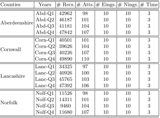
zero-one format. As a result the GB dataset comprised 110 items distributed over five dimensions: records, attributes, eastings, northings and time (months). Some statistics concerning the data sets are presented in Table 5.

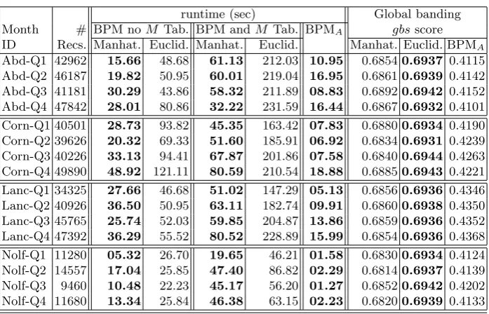
The results obtained are presented in Table 6 (best results highligted in bold font). Note that the table includes results from using and not using a BPM M-table (as considered in Section 4) and results using the BPMA algorithm presented previously in [1]. From the table the following can be noted: (i) using the BPMAalgorithm is more efficient than using BPM (Euclidean and Manhat-tan) (ii) not using BPM M-table requires less runtime than when using such a table (iii) using BPM with Manhattan weighting is more efficient than when using BPM with Euclidean weighting (because the use of Manhattan distances entail less calculation) and (iv) using BPM with Euclidean weighting produces the best bandings (gbsscores). Thus we can conclude that BPM with Euclidean weighting coupled with the use of a M-table is the most effective approach to the banded pattern mining problem. Closer inspection of the table also indicates that, as expected, there is a correlation between the number of records in the

2

data sets and the run-time; as the number of records increases the processing time increases (this is to be expected). Note that the BPMAalgorithm does not necessarily find a best banding but only an approximation because it does not consider the entire data space when calculating bandings (it only consider dimen-sion pairings). The BPM algorithm presented in this paper is designed to find an exact banding, instead of considering only dimension pairings as presented in [1], the bandings are derived with respect to the entire data space.

Table 5.Number of items in each dimension (after discretization) for the 16 5-D GB cattle movement data sets

Counties Years # Recs. # Atts. # Eings. # Nings. # Time

Aberdeenshire

Abd-Q1 42962 98 10 10 3

Abd-Q2 46187 101 10 10 3

Abd-Q3 41181 104 10 10 3

Abd-Q4 47842 107 10 10 3

Cornwall

Corn-Q1 40501 101 10 10 3

Corn-Q2 39626 104 10 10 3

Corn-Q3 40226 107 10 10 3

Corn-Q4 49890 110 10 10 3

Lancashire

Lanc-Q1 34325 97 10 10 3

Lanc-Q2 40926 100 10 10 3

Lanc-Q3 45765 103 10 10 3

Lanc-Q4 47392 106 10 10 3

Norfolk

Nolf-Q1 11526 98 10 10 3

Nolf-Q2 14311 101 10 10 3

Nolf-Q3 9460 104 10 10 3

Nolf-Q4 11680 107 10 10 3

7

Conclusion

Table 6.Runtime (RT) andgbsresults obtained using: (i) Manhattan and Euclidean BPM and no M-Table (ii) Manhattan and Euclidean BMP and M-Table and (iii) BPMA

runtime (sec) Global banding Month # BPM noM Tab. BPM andM Tab. BPMA gbsscore ID Recs. Manhat. Euclid. Manhat. Euclid. Manhat. Euclid. BPMA Abd-Q1 42962 15.66 48.68 61.13 212.03 10.95 0.68540.6937 0.4115 Abd-Q2 46187 19.82 50.95 60.01 219.04 16.95 0.68610.6939 0.4142 Abd-Q3 41181 30.29 43.86 58.32 211.89 08.83 0.68920.6942 0.4152 Abd-Q4 47842 28.01 80.86 32.22 231.59 16.44 0.68670.6932 0.4101 Corn-Q1 40501 28.73 93.82 45.35 163.42 07.83 0.68800.6934 0.4190 Corn-Q2 39626 20.32 69.33 51.60 185.91 06.92 0.68340.6931 0.4239 Corn-Q3 40226 33.13 94.41 67.87 201.86 07.58 0.68400.6944 0.4263 Corn-Q4 49890 48.92 121.11 80.59 210.54 18.88 0.68850.6943 0.4221 Lanc-Q1 34325 27.66 46.68 51.02 147.29 05.13 0.68560.6936 0.4346 Lanc-Q2 40926 36.50 50.95 63.11 182.74 09.91 0.68600.6938 0.4350 Lanc-Q3 45765 25.74 52.03 59.85 204.87 13.86 0.68590.6936 0.4352 Lanc-Q4 47392 36.29 55.52 80.52 228.89 15.99 0.68540.6936 0.4368 Nolf-Q1 11280 05.32 26.70 19.65 46.21 01.58 0.68300.6934 0.4124 Nolf-Q2 14557 17.04 25.85 47.40 86.82 02.29 0.68140.6937 0.4139 Nolf-Q3 9460 10.48 22.23 45.17 56.20 01.27 0.68520.6942 0.4202 Nolf-Q4 11680 13.34 25.84 46.38 63.15 02.23 0.68200.6939 0.4133

References

1. F. B Abdullahi, F Coenen, and R. Martin. A scalable algorithm for banded pattern mining in multi-dimensional zero-one data. In In Proc. Data Warehousing and

Knowledge Discovery (DaWaK’14). Springer, LNAI, pages 391–404, 2014.

2. J. Atkins, E. Boman, and B. Hendrickson. Spectral algorithm for seriation and the consecutive ones problem. SIAM J. Comput., 28:297–310, 1999.

3. A. Banerjee, C. Krumpelman, J. Ghosh, S. Basu, and R. Mooney. Model-based overlapping clustering. In Proceedings of Knowledge Discovery and DataMining, pages 532–537, 2005.

4. F. Coenen. LUCS-KDD ARM DN software. http:// www.csc.liv.ac.uk / frans/KDD /Software / LUCS KDD DN ARM/, 2003.

5. A. E. Cuthill and J. McKee. Reducing bandwidth of sparse symmetric matrices.

InProceedings of the 1969 29th ACM national Conference, pages 157–172, 1969.

6. C. Frans. LUCS-KDD Data generator software. http:// www.csc.liv.ac.uk / frans /KDD /Software / LUCS KDD DataGen Generator.html, 2003.

7. G .C Gemma, E. Junttila, and H. Mannila. Banded structures in binary matrices.

Knowledge Discovery and Information System, 28:197–226, 2011.

8. E. Junttila. Pattern in Permuted Binary Matrices. PhD thesis, 2011.

9. E . Makinen and H. Siirtola. The barycenter heuristic and the reorderable matrix.

Informatica, 29:357–363, 2005.

10. H. Mannila and E. Terzi. Nestedness and segmented nestedness. InProceedings of the 13h ACM SIGKDD international conference on knowledge discovery and data