________________________
New Trends in Stochastic Modeling and Data Analysis (pp. 159-171) Raimondo Manca – Sally McClean – Christos H Skiadas (Eds)
© 2015 ISAST
heterogeneous population composed of
subpopulations following the exponential law
Demetris Avraam1, Joao Pedro de Magalhaes2, Séverine Arnold (-Gaille)3 and Bakhtier Vasiev1
1
Department of Mathematical Sciences, University of Liverpool, Liverpool, UK (E-mail: [email protected] and [email protected])
2
Integrative Genomics of Ageing Group, Institute of Integrative Biology, University of Liverpool, Liverpool, UK
(E-mail: [email protected]) 3
Department of Actuarial Science, Faculty of Business and Economics (HEC Lausanne), University of Lausanne, Lausanne, Switzerland
(E-mail: [email protected])
Abstract. Many features of biological populations can be described in terms of their heterogeneity by taking into account variations among individuals and cohorts in the population. In demography, the heterogeneity of populations can explain various features of age-dependent demographic observations including those related to mortality dynamics. Mortality dynamics is underlined by the Gompertz law stating that the mortality rate increases exponentially between sexual maturity and considerably old ages (i.e. between 20 and 80 years old). Deviations from the exponential increase are observed at early- and late-life intervals. Different models (i.e Heligman-Pollard model) were developed over the past decades to describe and explain these deviations. These models postulate that a few different processes take place in the population and affect its mortality dynamics. In this study we present a model based on an assumption that mortality dynamics is indeed underlined by the exponential law and the irregularities at young and very old ages are due to the heterogeneity of human population. We demonstrate that the model is capable of reproducing the entire pattern of mortality and explaining the deviations from the exponential growth. The model fitted to Swedish age-dependent mortality rates indicates that the population should be composed of four subpopulations each following the exponential law of mortality increase over age. We also expand the idea of heterogeneity to probability density and survival functions, that is we adjust the model to the number of Swedish deaths and survivors instead of mortality rates.
1 Introduction
Analysis of the human mortality dynamics over the life-course is of great importance for many reasons including understanding the mechanisms of ageing and developing ways to control and extend the duration of lifespan. The mathematical modelling of the dynamics of human mortality makes a significant contribution to these studies. A number of studies have been performed to model (Makeham[21]; Siler[20]; Heligman and Pollard[12]; Lee and Carter[15]) and analyse (Gavrilov and Gavrilova[13]; de Magalhaes et al.[7]) mortality data as a function of age. Age-dependent mortality data are tabulated in life tables that contain essential information for the age-structure of a population (Preston
et al.[17]).
Two of the basic quantities of interest tabulated in a human life table are the probability of death and the mortality rate. Probability of death, qi, is the probability for an individual aged i to die before reaching age i+1 and is expressed as the ratio of the number of deaths of people aged ,i ∆Ni, divided by the number of individuals alive at exact age ,i Ni. Death (or mortality) rate
i
m is defined as the number of deaths of people of age i divided by the average number of individuals of age i:
1
(1) 0.5( )
i i
i i
N m
N N+
∆ =
+
where the number of deaths of people aged i is represented as:
1. (2)
i i i
N N N+
∆ = −
The average number of survivors within one-year age interval approximately coincides with the number of survivors at the centre of the interval and therefore the mortality rate is commonly referred as central death rate.
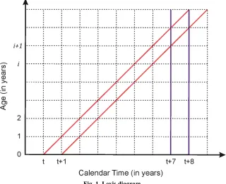
Fig. 1. Lexis diagram
The diagram illustrates demographic events as distributed over age and time. Cohort mortality rates refer to the deaths of a cohort that are occurring in a parallelogram formed by two diagonal lines. Period mortality rates refer to deaths occurring within a period outlined by two vertical lines.
The mortality rate of human populations (and other species as well) advances exponentially with age (i.e. follows the Gompertz law of mortality (Gompertz[1])) for a significant part of the age range starting from the period of reproductive maturity (age ~35) up to extreme old ages (age ~100). Mathematically, the Gompertzian dynamics of mortality is expressed as
0 , (3)
i i
m =m eβ
where m0 is the initial mortality at age i=0 and parameter
β
defines the rate of change of mortality with age (usually called rate of ageing or Gompertz slope).A number of mathematical models have been developed and used to analyse the human mortality dynamics and to clarify the deviations from the exponential growth. Various explanations have been given to the peculiarities of mortality at young and old ages. For example, the proposed explanations for the late-life mortality plateau include an assumption that the Gompertz law (exponential function) is not valid at those ages and that the mortality dynamics should be described by logistic, quadratic or some other mathematical functions (Gavrilov and Gavrilova[14]; Kannisto et al.[18]; Pham[5]). Other explanations take into account the heterogeneity of a population and its impact on the dynamics of mortality (Vaupel et al.[11]; Vaupel and Yashin[8]). The heterogeneity can be explained in different ways and can be described by different models (Lebreton[6]; Steinsaltz and Wachter[3]).
[image:4.595.151.446.305.530.2]
Fig. 2. Mortality rates of the 2010-period Swedish population set in a semi-logarithmic scale
The data are taken from the Human Mortality Database (http://www.mortality.org). The
Gompertz function with parameters m0=8.7 10⋅ −6 and
β
=0.109 fits the data very well after the age of 35. Deviations from the exponential growth are observed at young (before 35) and considerably old (after 100) ages.entire lifespan and are able to explain the deviations from the exponential growth. The model is fitted to Swedish period data and it is shown that a theoretical heterogeneous population composed by four subpopulations can reproduce the actual data fairly well. The model proposed in Avraam et al.[2], is then reformulated for the analysis of the probability density and survival functions of the population.
The remainder of this paper is structured as follows. In Section 2, the theoretical models in discrete and continuous age are introduced and their probability density and survival function for heterogeneous populations developed. Section 3 presents the fitting procedure we used. The models presented in Section 2 are applied to Swedish mortality rates in 2010 in Section 4 and obtained results are discussed in Section 5.
2 Mathematical model
2.1. Discrete model of mortality in heterogeneous populations
The main assumption of the model is that human populations are heterogeneous and composed of a number of subpopulations or individuals, which differ genetically and/or by life style factors (Vaupel et al.[10]; Vaupel[9]). The model that combines the heterogeneity with the Gompertz law of mortality (Avraam et al.[2]) has a further assumption that the mortality rate in each subpopulation grows exponentially (i.e. in the same way as in Gompertz law) with different mortality parameters (m0,β ) for each subpopulation, reflecting the variations in the genotype and life style. The notations Nj0, mj0
and
β
j are used for the initial size, initial mortality rate and rate of ageing of the j-th subpopulation respectively. The mortality or the central death rate of thej-th subpopulation at age i is then expressed by the exponential function:
0 j. (4)
i
ji j
m =m eβ
Using the definition of mortality rate (equation (1)), the mortality of the entire heterogeneous population composed by n subpopulations is given by:
1
, 1
1 1
, (5)
0.5
n
ji j i
n n
ji j i
j j
N m
N N
=
+
= =
∆ =
+
∑
∑
∑
0
1 0
0
1 1 0
1 0.5
. (6) 0.5 1 0.5 j j j j i n ji j i j j
i n n i
ji j
ji i
j j j
N m e m e m
N m e N m e β β β β = = = + = − +
∑
∑
∑
When dealing with period data the number of individuals aged i is constant for a stationary population and therefore the mortality rate is defined as the number of deaths ∆Ni divided by the actual size Ni. Thus, the model of mortality (equation (6)) for period data is simplified and can be expressed as a sum of weighted exponential terms:
1
0
1 1
1
, (7)
j n
ji n n
i j
i n ji ji ji j
j j
ji j
N
m m m e
N β ρ ρ = = = = ∆ = = =
∑
∑
∑
∑
where each weight
ρ
ji represents the proportion of the j-th subpopulation in the whole population at age :i1
with 1.
n ji ji ji i j N N ρ ρ = =
∑
=2.2. Continuous model of mortality in heterogeneous populations
In the continuous model the age is defined by a real number x
(continuous age) rather than by the integer number i. For continuous age, the instantaneous mortality, µx at age x (force of mortality) of a homogeneous population is defined as:
0
1
( ) lim . (8) ( ) ( )
x
N dN
x
N x x N x dx
µ
∆ →
−∆ −
= =
∆
Substituting the Gompertz law in the LHS of equation (8) and solving the differential equation results in:
0
( ) , (9)
x e
N x Ae
β
µ β − =
where the constant of integration A is equal to 0/
0
N eµ β as estimated by the initial condition N x( =0)=N0. This means that the expression for the population size N at age x depends on the initial mortality, µ0, and the mortality coefficient
β
:(
)
0 1
0
( ) . (10)
x e
N x N e
β
µ
β −
With heterogeneous populations, formula (10) is used to describe the size of each subpopulation at age x. Therefore, the subscript j is added in each parameter. As a result, the mortality of the entire population in continuous age is formulated by:
0
0
( / )(1 )
0 0
1 1
( / )(1 ) 0
1 1
( ) ( )
( ) . (11)
( )
x j
j j j
x j
j j
n n
x e
j j j j
j j
n n
e
j j
j j
x N x e N e
x
N x N e
β
β
β µ β
µ β µ µ µ − = = − = = = =
∑
∑
∑
∑
By solving equation (11) at integer values of age (x=i), equation (6) is found, providing then a link between the dynamics of mortality in the continuous and discrete models.
2.3. Probability density and survival function in heterogeneous populations
The consideration of heterogeneity in human population can be used for the derivation of models for other mortality-related variables that exist in human life tables. Such variables are the number of survivors and the number of deaths at age .x In this section, the models of probability density and survival function for heterogeneous populations are developed in continuous time.
In a homogeneous population, S x( + ∆x) denotes the probability of an individual to survive at age x+ ∆x (usually called survival function) and is calculated as the difference between the probability to survive at age x and the probability to die between x and x+ ∆x:
( ) ( ) ( ) ( ) (12)
S x+ ∆ =x S x −S x µ x∆x
( ) ( )
( ) ( ). (13)
S x x S x
x S x
x µ
+ ∆ −
⇒ = −
∆
The limit of LHS of equation (13) when ∆x tends to 0, is the derivative of S x( ) with respect to x:
0
( ) ( ) ( )
lim , (14)
x
S x x S x dS x
x dx
∆ →
+ ∆ − = ∆
and therefore equation (13) can be written as the differential equation ( )
( ) ( ). (15)
dS x
x S x dx = −µ
The solution of the differential equation (15) when the force of mortality µ( )x
follows the Gompertz law, is
0
( ) exp x , (16)
S x A µ eβ
β
= −
where the constant of integration A, is given by the initial condition ( 0) 1
By multiplying the survival function with the initial size of the population N0, we find the number of individuals alive at age x. Therefore, for the heterogeneous population, the theoretical number of survivors at age x is given by:
(
)
0
0 0 0
1
( ) ( ) exp 1 j . (17)
n x j j j j
N x N S x N ρ µ eβ
β = = = −
∑
The probability density function f x( ), of a heterogeneous population is obtained similarly. The probability q x( ) of an individual to die by age x is the complement of the probability to survive at the same age (i.e
( ) 1 ( )
q x = −S x ) and therefore the probability density function is obtained by differentiating the cumulative distribution function q x( ) with respect to x:
(
)
0 0
( ) '( ) exp x 1 . (18)
f x q x µ βx µ eβ
β
= = − −
By multiplying the probability density function with the size of the initial population, we have the theoretical distribution of deaths across the lifespan,
0
( ) ( ).
N x N f x
∆ =
For the case of a heterogeneous population composed by n
subpopulations, the distribution of deaths is given by the sum of the number of deaths of individuals from each subpopulation:
(
)
0
0 0 0 0
1 1
( ) ( ) exp j 1 . (19)
n n
x j
j j j j j
j
j j
N x N f x N ρ µ β x µ eβ
β = = ∆ = = − −
∑
∑
3 Fitting Procedure
The practical and commonly-used Least Squares Method was performed for the estimation of the model parameters that minimize the sum of the squared residuals between the theoretical and observed values. Log-Linear regression was used for the comparison between the logarithm of actual mortality rates and the logarithm of the theoretical mortality rates (logarithm of equation (6) or (11)), while Linear-regression was used to compare the actual number of deaths and survivors with the theoretical number of deaths given by equation (19) and theoretical number of survivors given by equation (17) respectively. In order to select the model with the optimal number of subpopulations, we used the Bayesian Information Criterion (BIC) (Schwarz[4]) which is given by the formula
( )
2( )
ln ln , (20)
d e d
BIC=n σ) +k n
ageing and its size or proportion with respect to the whole population) and also the sum of the subpopulations fractions is equal to unity. Therefore, the model of heterogeneous population composed by n subpopulations contains
3 1
k= n− unknown parameters.
4 Results
The theoretical heterogeneous population model is fitted to three different sets of mortality-related data (mortality rates, number of deaths and number of survivors) for the 2010 period Swedish data for the entire population including males and females. The data come from the website of Human Mortality Database, (http://www.mortality.org). We first fit the model to the mortality rates introduced in Fig. 2.
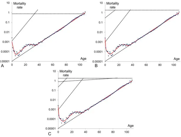
Fig. 3. The model of heterogeneous population fitted to the 2010 Swedish mortality rates
[image:9.595.144.451.317.549.2]The heterogeneous population composed by three (panel A), four (panel B) and five (panel C) subpopulations are presented. The observed mortality rates are denoted by the dot points, the mortality dynamics of the subpopulations are given by the dashed lines and the total mortality of the whole population by the solid curve.
(BIC= −315.73). In the four-subpopulation model (Fig. 3B), the first subpopulation considered as the frailest (the subpopulation with the highest initial mortality) explains the sharp decline of mortality pattern at infant ages. The second subpopulation (with initial mortality closed to 0.3) mainly forms the left part of the local minimum that is observed at young ages (ages 2-7). The third subpopulation with initial mortality around 0.001 forms the local hump that appears over the reproductive period (ages 20-30). This hump is frequently called the accidental hump since it reflects external death factors such as accidents (for both sexes) and maternal mortality (for females). The fourth subpopulation is the most robust (having the lowest initial mortality) and has the biggest initial fraction. It explains the exponential growth of mortality at the period of ageing.
The fitting procedure is then applied to the numbers of deaths and survivors taken for the 2010 Swedish population, with equation (19) and equation (17) respectively. The BIC values indicate that the best fit to the observed numbers of deaths and survivors is obtained in both cases with a model composed by four subpopulations (Fig. 4).
Fig. 4. The model of heterogeneous population fitted to the 2010 Swedish number of deaths and number of survivors
A: The density function of heterogeneous population composed by four subpopulations is fitted to the actual numbers of deaths and B: The survival function of heterogeneous population composed by four subpopulations is fitted to the actual numbers of survivors.
migration where the number of persons alive at age i+1 (Ni+1) in year t are equivalent to the number of persons alive at age i in year t−1 minus the number of persons who died at age i in year t−1, Ni− ∆Ni. However, since we do not fit cohort data but period data and since the Swedish population is subject to migration flows, this relation does not hold, explaining partly the observed differences between the values of the parameters of the three fitted models. The mortality rates of the entire population resulting from the model applied to the three different sets of Swedish data are shown in Fig. 5. The dotted and dashed curves indicate that the parameters obtained by fitting the numbers of deaths and survivors, fail to accurately model the peculiarities of mortality pattern at early and extreme old ages. However they both create a smooth dip at around age 75 and thus better capture the mortality pattern at adult age than the curve of mortality obtained by fitting mortality rates (solid curve in Fig. 5).
[image:11.595.149.447.335.562.2]
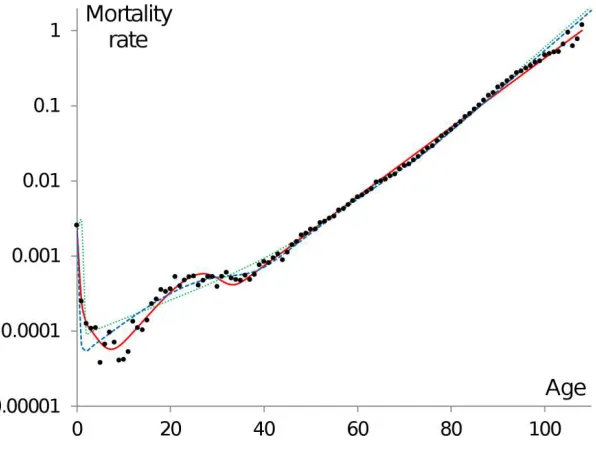
Fig. 5. Different fits of four-subpopulation heterogeneous model to 2010 Swedish mortality data
The solid (red) curve represents the mortality pattern resulting from the heterogeneous model fitted to the mortality rates (same pattern as in Fig. 3B) while the dotted (green) and dashed (blue) curves show the mortality pattern resulting from the model fitted to the numbers of deaths and the numbers of survivors respectively. (For interpretation of the references to colour in this figure legend, the reader is referred to the electronic version of this book.)
Modelling the dynamics of human mortality has long been the focus of various studies aiming an understanding the ageing processes and the causes of mortality at different ages. A number of studies have assessed the impact of heterogeneity on the dynamics of mortality, in particular at young and extremely old ages. The assumption that the population is heterogeneous combined with the assumption that the mortality dynamics of each subpopulation follows the exponential law, have been used to model the observed mortality dynamics and particularly to explain the deviations of mortality dynamics from the exponential growth (Avraam et al.[2]). In this work, we extended the model developed in Avraam et al.[2], from discrete to continuous time and we use it to reproduce and analyse the mortality dynamics across the entire human lifespan. The model contains meaningful demographic parameters and is capable of reproducing the actual data of a human population fairly well. The heterogeneity of a population is also used to derive models reproducing the patterns formed by the numbers of deaths and survivors.
The model reveals that we need to consider only four subpopulations to reproduce with sufficient accuracy the Swedish period mortality-related data (Fig. 3B and 4). The four-subpopulation model appears to be the optimum in all three fitted models we developed, that are 1) fitted model to mortality rates, 2) fitted model to the number of deaths and 3) fitted model to the number of survivors. Even though it probably underestimates the real heterogeneity of human populations, it shows how a simple mathematical model can well represent actual human mortality dynamics. Our analysis indicates that the contribution of heterogeneity differs across ages. The mortality model suggests that a small subpopulation with high initial mortality explains the decline in mortality at young ages as this subpopulation gradually disappears. Generally, the faster-ageing subpopulations are eliminated with increasing age and the entire population starts to act more-and-more homogeneously, as if it was composed by a single (with the lowest mortality) subpopulation.
References
1. B. Gompertz, On the Nature of the Function Expressive of the Law of Human Mortality, and on a New Mode of Determining the Value of Life Contingencies, Philosophical Transactions of the Royal Society of London, 115, 513–585, 1825. 2. D. Avraam, J.P. de Magalhaes and B. Vasiev, A mathematical model of mortality
dynamics across the lifespan combining heterogeneity and stochastic effects, Experimental Gerontology, 48, 801-811, 2013.
3. D.R. Steinsaltz and K.W. Wachter, Understanding mortality rate deceleration and heterogeneity, Mathematical Population Studies, 13, 19-37, 2006.
4. G. Schwarz, Estimating dimension of a model, Annals of Statistics, 6, 461-464, 1978. 5. H. Pham, Modeling US Mortality and Risk-Cost Optimization on Life Expectancy,
IEEE Transactions on Reliability, 60, 125-133, 2011.
6. J.D. Lebreton, Demographic models for subdivided populations: The renewal equation approach, Theoretical Population Biology, 49, 291-313, 1996.
7. J.P. de Magalhaes, J.A.S. Cabral and D. Magalhaes, The influence of genes on the aging process of mice: A statistical assessment of the genetics of aging, Genetics, 169, 265-274, 2005.
8. J.W. Vaupel and A.I. Yashin, The deviant dynamics of death in heterogeneous populations, Sociological Methodology, 15, 179-211, 1985.
9. J.W. Vaupel, Biodemography of human ageing, Nature, 464, 536-542, 2010. 10.J.W. Vaupel, J.R. Carey, K. Christensen, T.E. Johnson, A.I. Yashin, N.V. Holm, I.A.
Iachine, V. Kannisto, A.A. Khazaeli, P. Liedo, V.D. Longo, Y. Zeng, K.G. Manton and J.W. Curtsinger, Biodemographic trajectories of longevity, Science, 280, 855-860, 1998.
11.J.W. Vaupel, K.G. Manton and E. Stallard, Impact of heterogeneity in individual frailty on the dynamics of mortality, Demography, 16, 439-454, 1979.
12.L. Heligman and J.H. Pollard, The age pattern of mortality, Journal of the Institute of Actuaries, 107, 49-80, 1980.
13.L.A. Gavrilov and N.S. Gavrilova, The quest for a general theory of aging and longevity, Science of aging knowledge environment: SAGE KE 2003: RE5, 2003. 14.L.A. Gavrilov and N.S. Gavrilova, The reliability theory of aging and longevity,
Journal of Theoretical Biology, 213, 527-545, 2001.
15.R.D. Lee and L.R. Carter, Modelling and forecasting U.S. mortality, Journal of the American Statistical Association, 87(419), 659-671, 1992.
16.S. Gaille, Forecasting mortality: when academia meets practise, European Actuarial Journal, 2(1), 49-76, 2012.
17.S. Preston, P. Heuveline and M. Guillot, Demography: Measuring and Modeling Population Processes, Blackwell, Oxford, 2000.
18.V. Kannisto, J. Lauritsen, A.R. Thatcher and J.W. Vaupel, Reductions in mortality at advanced ages – several decades of evidence from 27 countries, Population and Development Review, 20, 793-810, 1994.
19.W. Lexis, Einleitung in die Theorie der Bevölkerungs-Statistik, Strassburg: Karl J. Trübner, 1875.
20.W. Siler, Parameters of mortality in human populations with widely varying lifespans, Statistics in Medicine, 2, 373-380, 1983.