Universities of Leeds, Sheffield and York
http://eprints.whiterose.ac.uk/
This is an author produced version of a paper published in Journal of the
Acoustical Society of America.
White Rose Research Online URL for this paper:
http://eprints.whiterose.ac.uk/9167/
Published paper
Zhang, J., Drinkwater, B.W. and Dwyer-Joyce, R.S. Ultrasonic oil-film
thickness measurement: An angular spectrum approach to assess performance
limits. Journal of the Acoustical Society of America, 2007, 121(5), 2612-2620.
Title:
Ultrasonic oil-film thickness measurement: an
angular spectrum approach to assess performance
limits
Authors and Addresses:
Jie Zhang1, Bruce W. Drinkwater1 and Rob S. Dwyer-Joyce2
1Department of Mechanical Engineering, University Walk,
University of Bristol, Bristol BS8 1TR, UK, email: [email protected]
2 Department of Mechanical Engineering, Mappin Street,
University of Sheffield, Sheffield S1 3JD, UK
Short Title:
Ultrasonic oil-film thickness measurement
Keywords:
Abstract
The performance of ultrasonic oil-film thickness measurement is explored. A ball
bearing (type 6016, shaft diameter 80 mm, ball diameter 12.7 mm) is used with a
50 MHz focused ultrasonic transducer mounted on the static shell of the bearing and
focused on the oil film. In order to explore the lowest reflection coefficient and hence
the thinnest oil-film thickness that the system can measure, three kinds of lubricant
oils (Shell T68, VG15 and VG5) with different viscosities were tested. The results
show a minimum reflection coefficient of 0.07 for both oil VG15 and VG5 and 0.09
for oil T68. This corresponds to an oil-film thickness of 0.4 µm for T68 oil. An
angular spectrum approach is used to analyse the performance of this configuration.
The effect of the key measurement parameters (transducer aperture, focal length and
centre frequency) is quantified. The simulation shows that for a focused transducer
the reflection coefficient tends to a finite value at small oil-film thickness. For the
transducer used in this paper the limiting reflection coefficient is shown to be 0.05
and that the oil-film measurement errors increase as the reflection coefficient
approaches this value. The implications for improved measurement systems are then
I. INTRODUCTION
The function of lubricant oil in a machine element such as a bearing is to control
friction and wear and hence provide smooth running and a satisfactory life. A large
amount of recent lubrication research is devoted to the study, prevention and
monitoring of oil degradation [1]. Lubricant degradation in service can lead directly
to machine element damage and machinery failure and so on-line monitoring is
desirable. The oil-film thickness gives information about the operating condition of
the oil and early warning of lubrication failure [2], allowing life prediction or
maintenance scheduling.
When an ultrasonic pulse strikes a very thin layer of lubricant (referred to in this
paper as the oil-film) in a bearing system, the film behaves mechanically as likes a
spring [3]. The reflected ultrasonic pulse is then a function of the oil-film stiffness,
which in turn depends on the oil-film thickness and its elastic properties. In this way
a simple spring-layer model can be used to extract oil-film thickness from the
measured reflection coefficient. Dwyer-Joyce et al. [3] and Zhang et al. [4] used this
technique to monitor the oil-film thickness in bearings such as journal bearings,
thrust-pad bearings and ball bearings. The results were shown to agree well with
models of the bearing performance. The thinnest oil-film thickness measured was
about 0.4 µm (corresponding to a reflection coefficient, R = 0.09) for Shell T68
engine oil in a 6016 ball bearing system [4]. There is significant interest in measuring
even thinner oil-films as much lubrication occurs under boundary lubrication
conditions which leads to oil-film thicknesses in the range 1-100 nm [1]. If very low
reflection coefficients (which correspond to very thin oil-films) could be measured
measurement devices.
In this paper, the angular spectrum technique is used to analyse the ultrasonic
measurement of oil-films. The angular spectrum approach uses a spatial Fourier
transform to decompose an arbitrary ultrasonic field into its component plane waves
[5]. These plane waves, which propagate at different angles, can then be analysed
separately and eventually recomposed into an ultrasonic field by an inverse angular
spectrum. The use of the angular spectrum to model the propagation of acoustic
fields and the output of transducers has been widely considered [6-10]. A number of
authors have also used the angular spectrum approach in conjunction with
multi-layered system models. For example Atalar [11] used the angular spectrum method to
analyse the performance of acoustic microscopes. He used various simple angular
dependent reflection coefficient functions to represent the interaction of the acoustic
microscope beam with a surface. Moidu et al. [12] used a similar approach to model
the inspection of adhesively bonded joints using planar and focused transducers. The
adhesive joint was modelled using a spring model of the interface and showed good
agreement with a number of normal and oblique incidence experiments. Croce et al.
[13] extended this analysis by using a full multi-layered system model.
In this paper, the angular spectrum approach is used to model the output from highly
focused ultrasonic transducers and the interaction of the resultant acoustic fields with
a thin oil-film. The primary aim is to quantify the performance of this measurement
system and assess the effect of transducer parameters such as aperture, focal length
and centre frequency. Experimentally, a minimum measurable oil-film reflection
transducer configuration however it should be noted the approach presented is
generally applicable.
II. BACKGROUND THEORY
II.A Ball bearing lubrication
For a ball bearing, operating in the elastohydrodynamic (EHD) lubrication regime, the
oil-film thickness can be determined numerically from the regression equations of
Dowson and Higginson [14]. They showed that the central film thickness, hc, can be
expressed as,
( )
(
m)
b c e R E n W E R E Uη R
h 0.73
067 . 0 2 ' ' 53 . 0 ' 67 . 0 ' ' 0
' 1 0.61
5 69 . 2 − − − ⎟⎟ ⎠ ⎞ ⎜⎜ ⎝ ⎛ ⎟ ⎠ ⎞ ⎜ ⎝ ⎛
= α (1)
where, U is the mean surface speed, η0is the lubricant viscosity at the contact entry,
and α is the pressure-viscosity coefficient, W is the radial load on the whole bearing
and nb is the number of balls, m is the ellipticity parameter, E′ is the reduced elastic
modulus and R′ is the reduced radius of curvature given by,
⎥ ⎦ ⎤ ⎢ ⎣ ⎡ − + − = ′ b b a a E E E 2 2 1 1 2 1
1 ν ν
,
by ay bx
ax R R R
R R 1 1 1 1 1 + + + =
′ (2)
where E is Young’s modulus, v is Poisson’s ratio. As shown in figure 1, the
subscripts a and b refer to the two rolling elements (i.e. the ball and the raceway) and
x and y refer to the co-ordinate axes. The contact area is elliptical in shape with the
3 1 2 30 / b a E n R nW m r ⎟⎟ ⎠ ⎞ ⎜⎜ ⎝ ⎛ ′ π ′ = , 3 1 30 / b b E m n R nW r ⎟⎟ ⎠ ⎞ ⎜⎜ ⎝ ⎛ ′ π ′
= (3)
where n is a measure of the shape of the contact ellipse. In this paper a 6016 ball
bearing was used and the parameters used in equations 1-3 are given in table 1 and the
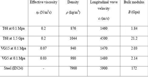
properties of the three oils used (T68, VG15, VG5) are shown in table 2. Note that
the properties at 1.5 GPa are extremely difficult to measure and so are only accurately
available for T68 oil [15].
II.B Reflection coefficient from an oil-film
Figure 2 shows a solid-lubricant layer-solid system, which represents the 3-layer
structure of a rolling element bearing. Surface 1 and 2 represent the bearing raceway
surface and ball surface, respectively. When an ultrasonic plane wave propagates
through this structure, ultrasound will be reflected from both the top and bottom
surfaces of the oil-film. However, as the oil-film is small compared to the wavelength
it is modelled as a boundary condition between the raceway and ball [16]. The
lubricant layer is then described by its normal and tangential stiffness, denoted by KN
and KT respectively. The normal stiffness of the lubricant layer can be simply related
to its thickness, h, and bulk modulus, B (where B = ρfcf2 and ρf is the density of the
lubricant layer and cf is the velocity of the longitudinal wave in the lubricant layer) by
[3],
h B KN =
(4)
respectively, and superscripts 1 and 2 represent the media. Of particular interest to
this paper are A1(l+), the incident longitudinal wave in medium 1 and A1(l-) the reflected
longitudinal wave in medium 1. In this notation the longitudinal wave reflection
coefficient in medium 1 is given by,
( )
[ ]
( ) ( )[ ]
+ − = l l A A R 1 1 ,θω (5)
Assuming that the solid half-spaces either side of the lubricant layer have identical
acoustic properties the amplitudes of the various plane waves are related by [16-18],
( ) ( ) ( ) ( )
[ ] [ ][ ]
( ) ( ) ( ) ( )⎪ ⎪ ⎭ ⎪ ⎪ ⎬ ⎫ ⎪ ⎪ ⎩ ⎪ ⎪ ⎨ ⎧ = ⎪ ⎪ ⎭ ⎪ ⎪ ⎬ ⎫ ⎪ ⎪ ⎩ ⎪ ⎪ ⎨ ⎧ − + − + − − + − + s s l l s s l l A A A A D S D A A A A 1 1 1 1 1 2 2 2 2 (6)where, [D] defines the relationship between the wave amplitudes and the normal and
shear stresses and displacements and [S] describes the spring boundary condition
between the two media. Matrices [D] and [S] are given by,
[ ]
⎥ ⎥ ⎥ ⎥ ⎥ ⎦ ⎤ ⎢ ⎢ ⎢ ⎢ ⎢ ⎣ ⎡ − − − − − − = s c s c C C C C s c s c C C c C C c C C sc C C sc C C sc C C sc C C c C C c D s s l l i s i s i s i s i s i s i l i l 1 1 2 2 2 2 1 2 1 2 2 2 2 2 2 2 2 2 2 2 β β β β (7)[ ]
⎥ ⎥ ⎥ ⎥ ⎥ ⎥ ⎦ ⎤ ⎢ ⎢ ⎢ ⎢ ⎢ ⎢ ⎣ ⎡ = 1 0 0 1 0 1 1 0 0 0 1 0 0 0 0 1 N T K Kwhere
(
)
2 1 2 21 1 c s
C = − l ,
(
)
21 2 2
2 1 c s
C = − s , 2 2
2 1 2c s
C β = − s , Ci =iωρ,
( )
( )
s s l l c cs= sinθ =sinθ
, ω is the centre frequency of the plane wave andθ is its incident
angle, defined with respect to the surface normal.
Note that for the case of a longitudinal wave, normally incident on a lubricant layer,
equations 4-8 can be simplified to calculate film thickness as [3],
2 2 1 2 ) ( R ) ( R Z B h n n ω ω ω −
= (9)
where, Z is the acoustic impedance of the media surrounding the lubricant film and
Rn(ω) is the amplitude of the normal incident plane wave reflection coefficient.
III. BALL BEARING EXPERIMENTAL APPARATUS
Figure 3(a) shows the experimental apparatus used to measure the ultrasonic
reflection coefficient from an oil-film in a 6016 ball bearing system. A rotating shaft
of 80 mm diameter was supported on four 6016 ball bearings lubricated via a total
loss gravity feed system. Bearings 1 and 4 were fitted to the ends of the shaft and
fixed into rigid housings. Vertically upwards radial loads were applied to the central
region of the shaft through bearings 2 and 3 via an arrangement of springs. This
meant that in bearings 1 and 4 the balls at the top of the raceway were the most
heavily loaded. The rotary shaft speed was controllable in the range 100-2900 rpm by
a 7.5 kWatt electric motor. This control of load and speed then enabled control of the
[image:9.595.83.512.72.152.2]An optical sensor was used, both to allow accurate triggering of the ultrasonic
instrumentation and to measure shaft speed. This was triggered by reflective tape
attached to the ball cage (which rotates at half the shaft speed). Bearing 1 was
instrumented with the ultrasonic measurement system that is shown in figure 3(b). A
focused, longitudinal wave piezoelectric ultrasonic transducer was mounted in the
housing such that it was normal to the top surface of the outer raceway. This
transducer acted as both an emitter and receiver (pulse-echo mode), and its parameters
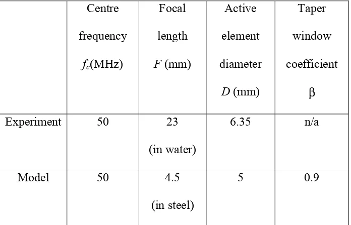
show in table 3. The transducer was focused on the outer raceway (4.5 mm thickness)
and designed to achieve a focal zone size smaller that the width of the lubricated
contact region. An ultrasonic pulser-receiver (Panametrics 5072PR) was used to
excite the ultrasonic transducer, receive and amplify the reflected signals which were
then passed to a digital scope (sampling frequency 5 GHz) and PC for storage and
analysis.
The reflective tape attached to the bearing cage is also shown in figure 3(b). When
this tape passed the optical sensor it generated a 5V positive trigger pulse. This pulse
was used to trigger a signal generator (Agilent 33220A). After the addition of an
adjustable delay the signal generator then triggered the pulser-receiver at its
maximum pulse repetition frequency, which was 20 kHz. By triggering in this way, a
number of ultrasonic pulses were able interrogate the lubricated contact region as it
passed under the transducer.
The reflection coefficient was measured by comparing the signal reflected from the
( ) )
( ) ( )
( ω
ω ω
ω ref
ref
m R
A A
R = (10)
where, Rref(ω) is the reflection coefficient of the reference interface, which in this case
was a steel-air interface obtained before the lubricant was introduced. This reflection
coefficient was then used in equation 9 to obtain the oil-film thickness.
Three oils with different viscosities (Shell T68, VG15, VG5) were used to explore the
minimum measurable oil-film thickness. In general, oils with lower viscosities
generate thinner oil-films for the same operating conditions (i.e. bearing load and
speed). For this reason it was thought that the lowest reflection coefficient would
result from the lowest viscosity oil.
IV. RESULTS
Figure 4 shows measurements of reflection coefficient for the three oils (Shell T68,
VG15, VG5) for a range of different operating speeds (w) and loads (W). From figure
4 it can be seen that the reflection coefficient decreases with increased load for all
oils. It can also be seen that for a given oil the reflection coefficient decreases as
speed decreases and that the lower viscosity oils exhibit lower reflection coefficients.
Qualitatively, all these trends follow the changes in oil-film thickness predicted by
equation 1, bearing in mind that a lower oil-film thickness is the cause of a lower
reflection coefficient. However, it can also be seen that the reflection coefficients
appear to reach a limiting value (of approximately 0.07) rather than tending to zero at
high load and low speed as equation 1 would suggest.
This section considers the effect of the transducer parameters such as aperture, D,
focal length, F, and centre frequency, fc, on oil-film thickness measurement by using
the angular spectrum approach. The spring-layer model (i.e. equations 5-8) is used to
model the wave interactions with the oil-film.
V.A Angular spectrum approach
The geometry of the measurement system used for the modelling is shown in figure 5.
For simplicity, the transducer is modelled as if it were directly coupled to the steel of
the bearing shell. This modelled transducer is then forced to focus on the lubricated
raceway-ball interface and so the need to model the propagation in the water is
removed. The aperture size is adjusted by a simple trigonometric calculation to
account for the small focussing effect in the water. In this way the 6.25 mm diameter
transducer with a focal length of 23 mm in water used experimentally (see table 3)
becomes a 5 mm diameter transducer of focal length in steel of 4.5 mm in direct
contact with the steel (see table 3). In figure 5, the planes labelled 1 and 2 represent
the modelled transducer plane and focal plane respectively and plane 2 is also the
plane of the oil-film. In the discussion that follows, the superscripts + and – refer to
fields propagating in the +z and –z directions, respectively.
The axial pressure of a focused circular transducer is given by [19] as,
⎥ ⎥ ⎥ ⎦ ⎤ ⎢ ⎢ ⎢ ⎣ ⎡ ⎟ ⎟ ⎟ ⎠ ⎞ ⎜ ⎜ ⎜ ⎝ ⎛ − + ⎟ ⎟ ⎠ ⎞ ⎜ ⎜ ⎝ ⎛ − + − −
= z a a D D z
a z p 4 4 sin 1
2 2 2 2
2
λ
π (11)
where, λ is the wavelength, a is the radius of curvature of the transducer, D is the
the distance at which pressure is a maximum then this equation can then used to
calculate the effective radius of curvature which results in the desired focal length (i.e.
4.5 mm in this case and equal to the bearing raceway thickness in general).
The displacement field at plane 1 due to the transducer is then modelled by the
following two dimensional windowing function,
( )
⎪ ⎪ ⎪ ⎪ ⎩ ⎪⎪ ⎪ ⎪ ⎨ ⎧ >= + < + < ⎥ ⎥ ⎦ ⎤ ⎢ ⎢ ⎣ ⎡ + ⎟ ⎟ ⎠ ⎞ ⎜ ⎜ ⎝ ⎛ + × <= + = + 2 0 2 2 1 2 / cos 5 . 0 2 when 1 , 2 2 2 2 2 2 2 2 1 D y x D y x D D y x D y x y x u β β π β (12)where the coefficient β defines the extent of the piston-like region of the transducer
(in this paper β=0.9). This taper was used to better represent a real transducer as well
as reducing the amplitude of the high spatial frequency components that result from
the use of a pure piston source (which is essentially a rectangular windowing
function). Following the approach of [6] the angular spectrum at plane 1 U1+(kx,ky) is
obtained by taking a spatial Fourier transform (denoted by FT) of the displacement
field,
(
)
(
(
)
)
∫ ∫
+∞(
)
(
(
)
)
∞ − +∞ ∞ − + + + = = ⋅ − + 1 1 1 1 1 1 1 1 1 11 k ,k FTu x,y u x,y exp jk x k y dxdy
U x y x y (13)
where kx and ky are the wavenumbers in the x and y directions respectively. In
practice equation 13 is implemented using a Fast Fourier Transform (FFT) routine on
an array of data representing the discretised spatial distribution of displacements.
1 to plane 2 (i.e. the focal plane),
(
)
(
)
⎟ ⎠ ⎞ ⎜ ⎝ ⎛ ⎟ ⎠ ⎞ ⎜ ⎝ ⎛ − + − ⋅ = ++ k ,k U k ,k j k k k F
U x y x y 2 x2 y2
0 1
2 exp (14)
where k0 is the wavenumber in the steel and
steel
c
k0 = ω . If it is assumed that all the
reflected ultrasound comes from the lubricated contact region then the reflected field
can be found from [6 and 12],
U −
(
kx,ky)
=U +(
kx,ky)
⋅R( )
ω,θ2
2 (15)
where, from equation 5, R(ω,θ) is the oil-film reflection coefficient for a plane wave
at an angle, θ, with respect to the normal of plane 2, ⎟⎟
⎠ ⎞ ⎜ ⎜ ⎝ ⎛ + = − 0 2 2 1 sin k k k
θ x y . A further
identical propagation term can then be used to simulate the propagation in the –z
direction back to plane 1 to give,
U
(
kx,ky)
U(
kx,ky)
j k kx ky F⎟⋅R( )
ω,θ⎠ ⎞ ⎜ ⎝ ⎛ ⎟ ⎠ ⎞ ⎜ ⎝ ⎛ − + ⋅ − ⋅ = +
− 2 2 2
0 1
1 exp 2 (16)
The acoustic field reflected back to plane 1 and hence received by the transducer is
then found by an inverse spatial FT of U1-(kx,ky),
( )
(
(
)
)
∫ ∫
+∞(
)
(
(
)
)
∞ − +∞ ∞ − − − − = = ⋅ + 1 1 1 1 1 2 1 1-1 , exp
4 1 ,
FT
,y U k k U k k j k x k y dxdy
x
u x y x y x y
π (17)
The amplitude recorded by the transducer, A, can then be calculated as the weighted
original transducer output, i.e. equation 12.
( ) ( )
( )∑
< + + − ⋅ = 2 2 2 2 x 11 , ,
D y y x u y x u
A (18)
Figure 6 shows a simulation of the measurement system obtained using this approach.
The acoustic properties of the media and transducer characteristics used in the
simulation are shown in table 2 and 3 respectively. A source plane (50×50 mm) was
defined with a spatial sampling interval of 25 µm (i.e. ∆x=∆y=25 µm). Figure 6(a)
shows the amplitude distribution at the focal plane (i.e. plane 2) obtained by equation
14 as well as the size of the lubricated contact region in a 6016 ball bearing for a
15 kN radial load from equation 3. From figure 6(a), it can be seen that the
assumption that the majority of the acoustic field is within the contact ellipse is
reasonable. Figure 6(b) shows the predicted reflection coefficient distribution and
weighted sum reflection coefficient for various oil-films. To generate this figure
equations 17 and 18 were used to calculate the displacement distribution and weighted
sum at the transducer. Simulations were performed for both the thin-film case and the
reference case (i.e. steel-air) and used in equation 10 to compute reflection coefficient
(using Rref = 1.0000). For the reflection coefficient distribution, equation 10 was
performed for each spatial point. In this way the model replicated the experimental
procedure. From figure 6(b) it can be seen that as the thickness of the oil-film
increases, so the reflection coefficient distribution becomes flatter and begins to
approach that of the weighted sum. It can also be seen from figure 6(b) that as the
oil-film thickness decreases so the acoustic field distribution (and hence the sum)
approach plateaux values. For example, oil-films of thickness 0.001 µm and
suggests that, for the particular transducer modelled there is a finite limiting reflection
coefficient below which measurement is not possible. This in turn implies a limiting
thickness as was observed experimentally in figure 4.
Simulations were performed for a range of oil-film thicknesses, and the weighted sum
reflection coefficient shown in figure 7(a), with a zoom of the important low thickness
region shown in figure 7(b). Also shown in these figures is the normal incidence
reflection coefficient (Rn) as a function of oil-film thickness. As the transducer is
mounted at normal incidence it would be standard practice to use the normal
incidence relationship to compute the oil-film thickness. For this reason the relative
difference between the reflection coefficient measured by a focused transducer and
the normal incidence plane wave reflection coefficient is defined as,
( ) ( )
( )
− ×100%=
n n wei
R h
R h R h
ε (19)
where, h(R) is the oil-film thickness obtained from equation 9, the normal incidence
spring model. From figure 7(b) it can be seen that the smallest measurable reflection
coefficient (labelled “Rlim”) for the simulated transducer is 0.05. Figure 7(c) shows
the relationship between the weighted sum reflection coefficient (Rwei) and the normal
incident reflection coefficient (Rn) (labelled “calibration line”). As the calibration line
departs from a line of unity gradient and zero intercept so the error between the
normal incidence plane wave and the focused transducer reflection coefficient
increases. For example, it can be seen from figure 7(c) that for a reflection coefficient
of 0.1 measured with the focused transducer, the resultant oil-film thickness
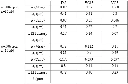
line shown in figure 7(c) could be used to compensate for this difference. As can be
seen from table 4 a reflection coefficient of 0.09 was measured for T68 oil at 15 kN
and 106 rpm and this corresponds to a 0.41 µm oil-film thickness. If the calibration
line in figure 7(c) is used to compensate for the focusing effect then the “effective”
normal incidence reflection coefficient becomes 0.07, which corresponds to a
0.31 µm oil-film thickness. Note that in this case the EHD model value obtained from
equation 1 is hc=0.27 µm. Similar results are shown in table 4 for the other oils. The
VG5 oil has the lowest viscosity of the three oils tested and so resulted in the thinnest
oil films (and therefore the lowest reflection coefficients). The calibration approach
described above has then been applied to the measured reflection coefficient data for
this oil and the result is shown in figure 4. For example from table 4 it can be seen
that at 15 kN and 106 rpm a reflection coefficient of 0.07 was measured which, after
calibration becomes 0.05. Although the acoustic properties of the VG5 oil under high
pressures are not accurately known, if a similar relationship between pressure, density
and bulk modulus is assumed then this minimum reflection coefficient equates to
hc=0.2 µm. This is therefore the thinnest oil-film yet measured using ultrasound and
this approach suggests a possible way forward to measure even thinner films. The
transducer parameters responsible for the effects described in this section are now
considered in more detail. In particular, experimental configurations which would
enable the measurement of even thinner films are considered.
V.B Variation of transducer parameters
For a transducer with F=4.5 mm and fc=50 MHz, figure 8 shows the limiting
levels of oil-film thickness error, Rε, (ε =2%, 5%, 10%) as a function of transducer
aperture. From figure 8, it can be seen that both Rlim and Rε increase with transducer
aperture, D. This is because a focused transducer with a large aperture size can be
thought of as emitting plane waves over a wide range of angles. Some of these plane
waves are then obliquely incident on the oil-film and are hence sensitive to a different
reflection coefficient than the normal incident plane waves. This implies that for
oil-film thickness measurement, the smaller aperture of the transducer, the better the
measurement. However, the aperture must be such that the focal zone size is smaller
than the lubricated contact.
For a given transducer aperture, D=5 mm and fc=50 MHz, figure 9 again shows Rlim
and Rε for various error cases (ε =2%, 5%, 10%), this time as a function of focal
length. From figure 9, it can be seen that both Rlim and Rεdecrease as the focal length
increases. As for the aperture the reason for this effect is that a focused transducer
with a long focal length emits plane waves over a smaller range of angles. This
implies that a large focal length is beneficial however, at 50 MHz the requirement for
a small focal zone size forces the choice of a focal length to be as small as possible
and hence equal to the bearing thickness.
For a given F=4.5 mm and D=5 mm, figure 10 shows Rlim and Rε for various error
cases (ε =2%, 5%, 10%) as function of centre frequency. From figure 10, it can be
seen that Rlim is almost constant (0.05). However it should be noted that according to
the spring-layer model (equation 9), a given reflection coefficient corresponds a
smaller film thickness at a higher frequency. Hence, the smallest measurable
From the analysis in this section, it can be seen that the ideal transducer for oil-film
thickness measurement would have a high centre frequency, a small aperture size and
long focal length. Figure 11 shows the performance of a possible transducer with
these features i.e. fc=150 MHz, D=1 mm and F=4.5 mm focal length. From this figure
it can be seen that it is possible to measure a reflection coefficient of 0.08 with 2%
error. This corresponds to a 0.12 µm oil-film thickness for T68 oil in a 6016 bearing
at 15 kN and 106 rpm.
VI. CONCLUSIONS
The use of a focused transducer to measure oil-film thickness has been shown to
generate errors if not approached with care. These errors increase as oil film
thickness decreases, potentially limiting the ability of ultrasound to measure very thin
oil-films. The angular spectrum approach has been used to model the measurement
system and the interaction of the resultant plane waves with a spring-layer. The
analysis showed that oil-film thickness measurement errors decrease as centre
frequency and focal length increase and transducer aperture decreases. For a specific
focused transducer (50 MHz centre frequency, focal length of 4.5 mm and aperture of
5 mm) the theoretical thickness measurement error was predicted to be 17% when the
measured reflection coefficient was 0.1, and a finite reflection coefficient limit was
reached at 0.05. This compared well with the experimentally observed reflection
coefficient limit of 0.07. A calibration approach was described which allowed an
oil-film thickness of 0.2 µm to be measured, thinner than had previously been possible.
For the T68 oil which has well known acoustic characteristics the experimental results
improved performance on very thin oil-films.
ACKNOWLEDGEMENTS
This work has been funded by the UK Engineering and Physical Sciences Research
Council under Grant No. GR/S046956/01.
REFERENCES
1. G.W. Stachowiak and A.W. Batchelor, Engineering Tribology (Butterworth
Heinemann, Woburn, MA, 2001).
2. J. Zhang, B.W. Drinkwater and R.S. Dwyer-Joyce, “Monitoring of lubricant film
failure in a ball bearing using ultrasound,” J. Tribol.-Trans. ASME 128, 622-618
(2006).
3. R.S. Dwyer-Joyce, B.W. Drinkwater and C.J. Donohoe, “The measurement of
lubricant-film thickness using ultrasound,” Proc. R. Soc. Lond. A. 459, 957-976
(2003).
4. J. Zhang, B.W. Drinkwater and R.S. Dwyer-Joyce, “The measurement of
lubricant-film thickness in rolling element bearings using ultrasound,” J. Acoust. Soc. Am.
119, 863-871 (2006).
5. J.W. Goodman, Introduction to Fourier optics, (McGraw Hill, New York, 1978).
6. P.R. Stepanishen and K.C. Benjamin, “Forward and backward projection of
acoustic fields using FFT methods,” J. Acoust. Soc. Am. 71, 803-812 (1994).
acoustic fields,” J. Acoust. Soc. Am. 90, 507-521 (1991).
8. D.P. Orofino and P.C. Pedersen, “Efficient angular spectrum decomposition of
acoustic sources – part I: theory,” IEEE Trans. Ultrason. Ferr. Freq. Cont. 40, 238-249
(1993).
9. C.J. Vecchio and P.A. Lewin, “Finite amplitude acoustic propagation modelling
using the extended angular spectrum method,” J. Acoust. Soc. Am. 94, 2399-2408
(1994).
10. P. Wu, R. Kazys and T. Stepinski, “Optimal selection of parameters for the
angular spectrum approach to numerically evaluate acoustic fields,” J. Acoust. Soc.
Am. 101, 125-134 (1997).
11. A. Atalar, “An angular-spectrum approach to contrast in reflection acoustic
microscopy,” J. Appl. Phys. 49, 5130-5139 (1978).
12. A.K. Moidu, A.N. Sinclair and J.K. Spelt, “Nondestructive characterization of
adhesive joint durability using ultrasonic reflection measurements,” Res. Nondestr.
Eval. 11, 81-95 (1999).
13. R. Croce, P. Calmon and L. Paradis, “Modeling of propagation and echo
formation in a multilayered structure,” Ultrasonics 38, 537-541 (2000).
14. D. Dowson and G.R. Higginson, Elasto-Hydrodynamic Lubrication (Pergamon
Press, New York, 1977).
15. O.B. Jacobson and A.P. Vinet, “Model for the influence of pressure on the bulk
lubricants,” J. Tribol.-Trans. ASME 109, 709-714 (1987).
16. T.P. Pialucha and P. Cawley, “The detection of thin embedded layers using
normal incidence ultrasound,” Ultrasonics 32, 431-440 (1994).
17. M.J.S. Lowe, “Matrix techniques for modelling ultrasonic waves in multilayered
media,” IEEE Trans. Ultrason. Ferr. Freq. Cont. 42, 525-542 (1995).
18. S.I. Rokhlin and Y.J. Wang, “Analysis of boundary conditions for elastic wave
interaction with an interface between two solids,” J. Acoust. Soc. Am. 89, 503-515
(1990).
19. H.T. O’Neil, “Theory of focusing radiators,” J. Acoust. Soc. Am. 21, 516-526
Tables
Table 1. Parameters used to calculate the theoretical oil-film thickness in a 6016 ball
bearing via equation 1 [14].
Reduced modulus
E′ (GPa)
Reduced radius
R′(m)
Pressure viscosity coefficient for T68
α(Gpa-1)
Ellipticity parameter
m
Simplified Elliptical Integrals
n
Effective viscosity for
T68
η0 (N/m2s)
Table 2. Acoustic properties of lubricant oils and steel.
Effective viscosity
η0(N/m2s)
Density
ρ (kg/m3)
Longitudinal wave velocity
cl (m/s)
Bulk modulus
B (Gpa)
T68 at 0.1 Mpa 0.2 876 1460 1.84
T68 at 1.5 Gpa 0.2 1044 4500 21.2
VG15 at 0.1 Mpa 0.07 940 1470 2.03
VG5 at 0.1 Mpa 0.03 980 1480 2.14
Table 3. Experimental and modelled transducer parameters.
Centre
frequency
fc(MHz)
Focal
length
F (mm)
Active
element
diameter
D (mm)
Taper
window
coefficient
β
Experiment 50 23
(in water)
6.35 n/a
Model 50 4.5
(in steel)
Table 4. Reflection coefficient and oil-film thicknesses for various oils and operating
conditions. Also shown are oil-film thickness values from EHD theory [14].
T68 VG15 VG5
R (Meas) 0.09 0.07 0.068
hc(µm) 0.41 0.31 0.3
R (Calib) 0.07 0.05 0.046
hc(µm) 0.31 0.22 0.2
w=106 rpm, L=15 kN
EDH Theory hc (µm)
0.27 0.14 0.07
R (Meas) 0.18 0.112 0.11
hc(µm) 0.81 0.5 0.49
R (Calib) 0.177 0.099 0.097
hc (µm) 0.8 0.44 0.43
w=506 rpm, L=15 kN
EDH Theory hc(µm)
List of Figures
Figure 1. Geometry of the contact between the outer-raceway of the bearing and ball.
Figure 2. Three-layer system model of the oil-film.
Figure 3. (a) Schematic diagram of the experimental apparatus made up of four 6016
ball bearings, (b) Transducer attachment and bearing geometry.
Figure 4. Experimentally measured reflection coefficients for three oils (T68, VG15
and VG5) at various operating condition Also shown is the calibrated reflection
coefficient for oil VG5.
Figure 5. Geometry of the focused transducer used for the angular spectrum
simulation.
Figure 6. Simulation results for the modelled transducer (defined in table 3). (a)
Amplitude distribution at the focal plane. (b) Reflection coefficient distribution along
the x-axis for a number of oil-film thicknesses.
Figure 7. Simulated reflection coefficient results from a range of oil-film thicknesses
by using the modelled transducer (defined in table 3). (a) Reflection coefficients as a
function of oil-film thickness. (b) Zoom in the left corner area in Figure 7(a). (c)
Calibration line.
Figure 8. Reflection coefficient as a function of transducer aperture, F=4.5 mm and
fc=50 MHz are assumed.
D=5 mm and fc=50 MHz are assumed.
Figure 10. Reflection coefficient as a function of centre frequency of the transducer,
F=4.5 mm and D=5 mm are assumed.
Figure 11. Theoretical error from a focused transducer with 1 mm aperture, 150 MHz