Proper Orthogonal Decomposition Analysis and Modelling of the
wake deviation behind a squareback Ahmed body
B´ereng`ere Podvin, St´ephanie Pellerin, and Yann Fraigneau LIMSI, CNRS, Universit´e Paris-Saclay
Antoine Evrard ENSTA
Olivier Cadot University of Liverpool (Dated: October 1, 2019)
Abstract
We investigate numerically the 3-D flow around a squareback Ahmed body at Reynolds
num-ber Re = 104. Proper Orthogonal Decomposition (POD) is applied to a symmetry-augmented database in order to describe and model the flow dynamics. Comparison with experiments at a
higher Reynolds number in a plane section of the near-wake at mid-height shows that the
simula-tion captures several features of the experimental flow, in particular the antisymmetric quasi-steady
deviation mode. 3-D POD analysis allows us to classify the different physical processes in terms
of mode contribution to the kinetic energy over the entire domain. It is found that the dominant
fluctuating mode on the entire domain corresponds to the 3-D quasi-steady wake deviation, and
that its amplitude is well estimated from 2-D near-wake data. The next most energetic flow
fluctu-ations consist of vortex shedding and bubble pumping mechanisms. It is found that the amplitude
of the deviation is negatively correlated with the intensity of the vortex shedding in the spanwise
direction and the suction drag coefficient. Finally, we find that despite the slow convergence of the
decomposition, a POD-based low-dimensional model reproduces the dynamics of the wake
devia-tion observed experimentally, as well as the main characteristics of the global modes identified in
the simulation.
I. INTRODUCTION
A surprisingly generic feature of the flow around symmetric bodies at high Reynolds numbers is the presence of permanent symmetry-breaking structures in the wake. These have been observed for the sphere [9], bullet [24] , the flat plate [2], as well as academic models for ground vehicles such as the Ahmed body [10] and the Windsor body [18]. The origin and dynamics of these structures has not been entirely elucidated, although they have been the object of several experimental and numerical studies. They appear to be connected to the first bifurcation observed at much lower Reynolds number (see [7], [8]). At higher Reynolds numbers, rapid switches between different quasi-stable states can be observed, as described by [22] and [1].
the Ahmed body that was able to reproduce the steady wake deviation. However switches were not observed in Pasquetti and Peres’s simulation, since the typical time separating two switches is on the order of 1000 U/H where U is the incoming flow speed and H the body characteristic height (see [14]). In more recent work Dalla Longa et al. [4] were able to integrate over sufficiently long times to capture the switch in the wake deviation. However they could only observe one switch, due to the still longer time scale separating two switches. They also applied Proper Orthogonal Decomposition and Dynamic Mode Decomposition (DMD, [25]) to extract the dynamics of the flow. Interaction of the near-wake recirculation zone with the surrounding shear layers is expected to play a part in the occurence of switches. They proposed that the switch is triggered by large hairpin vortices. Volpe et al. [28] carried out a spectral analysis of the wake behind the squareback Ahmed body. Three low frequencies were identified in their experimental data: vortex-shedding modes with Strouhal numbers of 0.13 and 0.19 in the far wake, and wake pumping motion at a Strouhal number of 0.08 in the recirculation zone. Paviaet al. [17] have applied POD to both the experimental pressure and velocity field of a Windsor body to identify structures corresponding to the bi-stable modes and the dynamics of the switch. They identified pumping motion in the wake with a bi-stable vortical structure in the streamwise direction and derived a phase-averaged model that describes the switch between the quasi-stable states. They confirmed the observation made by Evrard et al. [5] and Cadot et al. [2] that the symmetric state corresponds to a lower drag.
Drag reduction through control of the flow asymmetry has been the object of several passive and active control strategies [14], [29], [1], [13], [27], [6], [23]. An important question is to determine how the different structures present in the flow contribute to the drag. A low-dimensional description and modelling of the large-scale structures could be beneficial for understanding, predicting and ultimately controlling the flow dynamics. Reduced-order models were developed by [1], [22] in order to control the deviation of the wake.
How-ever, reflection symmetry was enforced artificially, so that we provide a description of the structures of the flow as a superposition of reflection-symmetric and reflection-antisymmetric modes.
The paper is organized as follows: section 2 presents the 3-D numerical configuration, while section 3 describes the specifics of Proper Orthogonal Decomposition. Section 4 presents a 2-D comparison of the numerical simulation and an experimental configuration corresponding to the same geometry but a higher Reynolds number, section 5 presents a 3-D POD analysis of the structures in the full configuration; a POD-based low-dimensional model is constructed in section 6 and compared with experimental and numerical results. A conclusion is given in section 7.
II. NUMERICAL CONFIGURATION
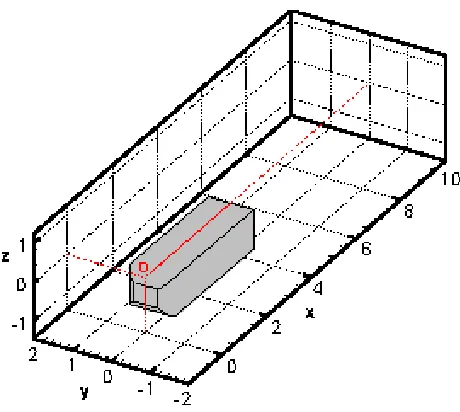
Figure 1 presents the numerical configuration. The dimensions of the squareback Ahmed body are the same as the experimental configuration of Evrard et al. [5] i.e. L = 1.124m, H = 0.297m, W = 0.35m. The ground clearance (distance from the body to the lower boundary of the domain) is 0.3H in the simulation. The Reynolds number based on the incoming velocity U, body height H and fluid viscosity is 104. The foremost and upper part body defines the reference position (x= 0, z = 0). The plane y= 0 corresponds to the mid-plane of the body. The domain extent in the streamwise (x), spanwise (y) and vertical (z) directions is [−1,10]H×[−2,2]H×[−1.3,1.2]H.
FIG. 1. Numerical configuration. The Ahmed body and the recirculation zone behind it are idenfied
by a surface of zero streamwise velocity. The streamwise, spanwise and wall-normal positions are
referred to as x, y, z. The length, width and height of the body are respectively L, W and H.
The origin of the axes is taken at the top and foremost position of the Ahmed body in the vertical
symmetry plane.
convergence to be reached. We note that all times will be expressed in those units in the remainder of the paper. All lengths will be made nondimensional with the body height H.
III. PROPER ORTHOGONAL DECOMPOSITION
The main tool of analysis used in this paper is Proper Orthogonal Decomposition (POD) [15]. The field on a domain Ω is written as a superposition of spatial modes
u(x, t) =X n
˜
an(t)φn(x) (1)
where the modes are orthogonal (and can be made orthonormal), i.e
Z
φn(x).φm(x)dx=δnm.
The modes can be ordered by decreasing energy λ1 ≥ λ2 ≥ . . . ≥ λn =< ˜an˜an >, where
< . > represents a time average. The amplitudes ˜an can be obtained by projection of the velocity field onto the spatial modes:
˜ an(t) =
Z
Ω
u(x, t).φ
In the remainder of the paper we will consider normalized amplitudes an= ˜an/ √
λn.
In all that follows POD is implemented following the method of snapshots [26] which is based on computing the autocorrelation between the different samples of the field obtained at timesti, i= 1, . . . , N:
Cij = 1 N
Z
Ω
u(x, ti).u(x0, tj)dx,
and extracting the eigenvalues λn and temporal eigenvectors Ain =an(ti) such that
CA=λA. (3)
The spatial modes can then be reconstructed using
˜ φ
n(x) =u(x, ti)Ain (4) and renormalizingφ
n(x) =
1
Nn
˜ φ
n(x) where
Nn2 =
Z
˜
φn(x).φ˜n(x)dx. (5)
Different spatial domains, as well as different quantities will be considered in the decom-position. In section 4, we will limit the analysis to 2-D velocity fields in the near-wake region in order to match the data of Evrard et al. [5]. In section 5, we will apply POD to the full 3-D velocity field to the full numerical domain.
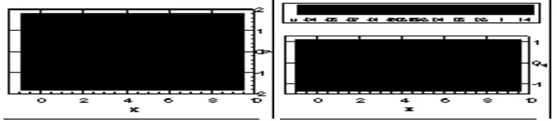
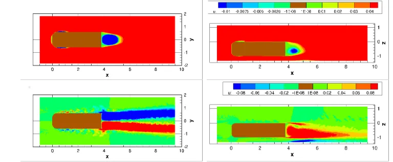
FIG. 2. Streamwise velocity contours of the mean flow; left) horizontal plane at mid-height
z=−0.5; right) vertical mid-plane atz= 0.
We emphasize that individual POD modes are different from coherent structures. A coherent structure typically corresponds to local patterns identified in a realization. POD modes are defined over the full domain chosen for decomposition, and every single realiza-tion contains a combinarealiza-tion of modes. A coherent structure will therefore correspond to a combination of a few POD modes, which may be restricted to a portion of a spatial domain. As a consequence of the data enlargement procedure we have adopted, the mean flow of the simulation does not correspond to one single mode but to the sum of the first two modes representing respectively the symmetric and the antisymmetric part of the mean flow.
IV. 2-D POD: COMPARISON WITH THE EXPERIMENT
In this section we apply POD analysis in the near-wake to the same variables defined over the same domain in both the experiment and the numerical simulation, i.e. the streamwise and the spanwise velocity components u et v defined over the domain L ≤ x ≤ L+ 1.2H, −0.6≤y≤0.6H. Details are indicated in table I. The main differences are
(i) the Reynolds numbers considered, as Re= 4 105 in Evrard’s experiment and Re= 104 in our numerical simulation
(ii) the time resolution - which is 25H/U in the experiment versus 0.5H/U in the simulation.
Type Re ∆T snapshot number (original data set)
Simulation 103 0.5 150
Experiment 4 105 25.25 400
TABLE I. Comparison between model and experiment
the experiment and the simulation. The second mode represents about 35% of the total fluctuating horizontal kinetic energy in the wakeP
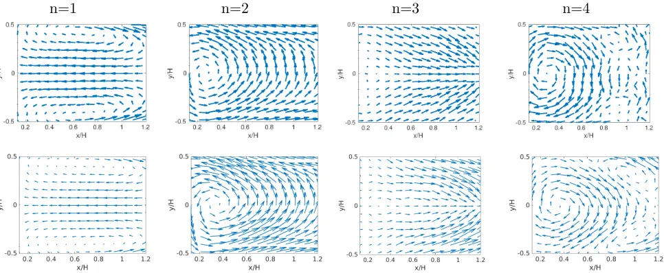
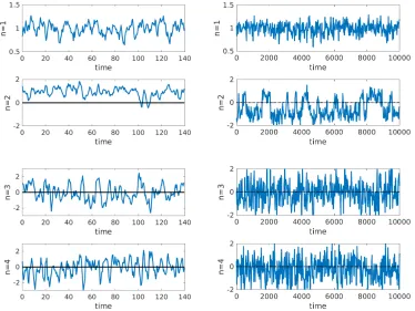
p≥2λp and the first eight modes capture more than 50%. Figure 4 compares the first four POD modes for the experiment and the simulation. The first mode represents a cross-section of a toroidal-like structure constituting the recirculation bubble. The second mode corresponds to a single vortical structure located in the recirculation bubble close to the rear of the body and sweeping fluid from one side of the wake to the other. It represents the wake deviation. Overall a good agreeement is observed between all the modes found in the experiment and those found in the simulation. Figure 5 shows for both the experiment and the simulation the corresponding amplitudes (normalized by the square root of the eigenvalue) of the modes represented in figure 4. The amplitudes of the first two modes in the simulation (figure 5 right) display small oscillations around a constant positive value. In the experiment (figure 5 left), the amplitude of the first mode oscillates near a constant positive value, while the amplitude of the second mode changes sign several times, which corresponds to a switch in the wake asymmetry.
We can also see from figure 4 that mode 3 is symmetric and mode 4 is antisymmetric. Mode 3 consists of a longitudinal converging (or diverging, depending on the sign of the amplitude) motion at the extremity of the recirculation bubble, which could be associated with wake pumping i.e successive enlargment and shrinking of the recirculation region. Mode 4 consists of three vortical structures - one larger structure extending across the wake and located close to the rear of the body, and two smaller ones, both rotating in the opposite direction, on each side of the recirculating bubble. Its action is therefore to distort the recirculation bubble in the spanwise direction. Since the PIV results are not resolved in time and the simulation total time is relatively short, it is difficult to compare directly time evolutions. However histograms of the amplitudes can be compared in figure 6 (we note that only the amplitudes corresponding to the original set of snapshots are shown). We can see that there is a relatively good agreement between the experiment and the simulation.
sug-FIG. 3. Near-wake 2-D POD spectrum in the simulation and experiment.
[image:9.612.201.445.77.270.2]n=1 n=2 n=3 n=4
FIG. 4. 2-D wake POD modes 1 to 4; top row: simulation; bottom row: experiment.
gests that the most energetic structures have common features over a wide range of Reynolds numbers.
[image:9.612.52.535.328.527.2]FIG. 5. Amplitudes of 2-D POD modes 1 to 4 (from top to bottom); left) simulation; right)
experiment.
mixture of frequencies.
V. 3-D POD
To investigate the flow structure and dynamics in more detail, POD is applied to the full 3-D velocity field over the entire computational domain. The eigenvalue spectrum is shown in figure 9. The first 3-D mode, which coincides with the mean flow, is much more energetic than the other modes compared with 2-D analysis (figure 3) since the entire domain contains a large steady contribution of the kinetic energy outside the wake. Due to the extent of the spatial domain, the convergence of the fluctuations is much slower than in the 2-D wake measurements. The second mode represents only 8% of the total fluctuating kinetic energy
P
[image:10.612.158.532.78.359.2]n=1 n=2 n=3 n=4
FIG. 6. Histogram comparison of 2-D POD modes 1 to 4 (from left to right); top row: simulation;
bottom row: experiment.
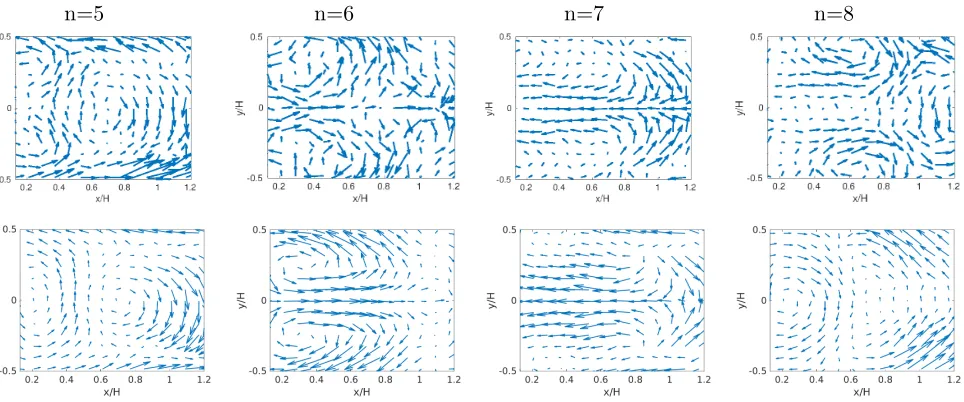
[image:11.612.97.557.78.274.2]n=5 n=6 n=7 n=8
FIG. 7. 2-D wake POD modes 5 to 8; top row: simulation; bottom row: experiment.
wake. Figure 10 shows the projection of an instantaneous velocity field on the first ten modes and the difference between the full field and its projection. It is clear that only the large scales are captured by the projection. One can see that most of the unresolved modes (which represent the major portion of the total kinetic energy) are located in the boundary layers, the shear layers and the far wake.
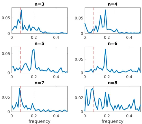
[image:11.612.55.537.345.546.2]FIG. 8. 2-D POD amplitude power spectral density |ˆan|2 for modes 3 to 8 - the red and black
dashed lines respectively correspond to the frequencies 0.08 and 0.2.
FIG. 9. 3-D POD eigenvalue spectrum.
[image:12.612.199.434.385.574.2]FIG. 10. Streamwise velocity contours on mid-height plane z =−0.5; top : projection of an
in-stantaneous fielduonto the first ten modesurecons=P10n=1an(t)φ(x) wherean=Ru(x, t).φ(x)dx.;
bottom: difference field |u−urecons|.
the 2-D POD results, which is not entirely surprising since they are expected to represent the symmetric and antisymmetric part of the time-averaged velocity field.
One can see in figure 12 that the temporal evolution of the first two 3-D POD modes is slightly different from that of the 2-D POD coefficients. Unlike its 2-D counter part (figure 5 right), the amplitude of the first 3-D POD mode is essentially constant, which shows the statistical convergence of the database. Moreover, the amplitudes of the second 2-D and 3-D mode present some discrepancies, but the correlation between the mean deviation co-efficient a2d
a local planar measure may indicate otherwise. In both cases, their corresponding spectrum indicates fluctuations at low frequencies thus confirming their very long-time dynamics evo-lution. In addition to its permanent asymmetry, the POD mode 2 corresponds to the very low frequency global mode as reported in [22, 23] for an axisymmetric body and responsible for the bistable dynamics found in [9] for the Ahmed body. To get a better insight into the action of the global deviation mode, figure 13 compares streamlines in the recirculation zone for the symmetrized mean field (mode 1) and the mean field (modes 1 and 2). We can see that the effect of the global deviation is to gather the streamlines around one of the base diagonals.
n=1
[image:14.612.136.520.268.426.2]n=2
FIG. 11. Streamwise velocity contours of 3-D POD modes 1 (top row) and 2 (bottom row); left)
horizontal section at mid-height z=−0.5; right) vertical section aty =−0.4.
FIG. 12. Left) amplitudes of the first two POD modes; right) power spectral density of the
quasi-steady deviation mode|ˆa2|2 - the red and black lines respectively correspond to the two frequencies 0.08 and 0.2.
FIG. 13. Streamlines of the field viewed from downstream left) mode 1√λ1φ1; right) combination of mode 1 and mode 2 √λ1φ1+
√
λ2φ2 .
[image:15.612.100.526.77.244.2]Rigas et al. [24], Volpe et al. [28] and Pavia et al. [17].
Modes 9 and 10, which are antisymmetric (figure 14), are more difficult to interpret. As noted earlier, there is no guarantee that an individual POD mode corresponds to a well-defined physical mechanism. The spectra in figure 15 (right) show that modes 9 and 10 are characterized by a mixture of frequencies in an intermediate range 0.08-0.2, with a peak for both modes around 0.15. It is therefore likely that these modes correspond to a superposition of different physical processes.
As a summary, we find a clear correspondance between the POD modes and the main global modes that contribute to the wake dynamics reported in the literature: POD mode 2 is related to the very low frequency asymmetric or deviation global mode, modes 3 and 4 to vortex shedding with oscillation in the horizontal direction, modes 5 and 6 to vortex shedding with oscillations in the vertical direction, and modes 7 and 8 to (symmetric) wake pumping.
The POD decomposition allows to investigate quantitatively the correlations between the global modes during the wake dynamics. We first compare the intensity of the deviation global mode given by (a2
2) with the magnitude of vortex shedding in the horizontal (spanwise) and the vertical direction which can respectively be obtained with the sums of the amplitudes r2
Kh =a23+a24 andrKv2 =a25+a26. We can see in figure 16 that minima ofa2 are associated with high energy in spanwise vortex shedding. The correlation coefficient between |a2| and |a3|2+|a4|2 is strongly negative (-0.6). Due to the three-dimensional nature of vortex shedding, spanwise and vertical shedding motions are correlated (0.48), so that a negative correlation is also obtained between |a2| and a25 +a26 (-0.33). The negative correlation is consistent with the idea that a reduced asymmetry is accompanied by an increase in vortex shedding, which was observed in control experiments of [1] and [13].
The next step is to compare the evolution of the POD amplitudes with the base suction coefficient CB =−Cpb where the pressure coefficient Cpb corresponds to the integral of the pressure over the base of the body, which is shown in figure 17 (left). Figure 17 (right) shows that the base suction coefficient is positively correlated with the amplitude of the wake deviation a3d
2 with a positive delay of ∆tU/H ∼2.5 and with a maximum correlation coefficient of 0.55 ( we note that the correlation coefficient with the 2-D deviation mode a2d
the drag follow those of the mean deviation amplitude. This is in agreement with the idea that a drag reduction corresponds to a decrease in the quasi-steady wake asymmetry, as was observed by [2] and [17]. Figure 17 also shows that a correlation coefficient of -0.55 with a negative delay of ∆tU/H ∼ −1.5 is observed between the pressure and the amplitude of a7. Unlike the previous case, the correlation remains about the same without no time delay (-0.51), so it is not possible to assign a physical relevance to the small time delay observed. As seen above, a7 is associated with wake pumping: from figure 14 one can see in the near-wake that when a7 > 0 there are more negative fluctuations within the zone, so that the size of the recirculation actually increases. This is consistent with the observation that the base suction coefficient decreases as the recirculation length increases.
In contrast, the correlation of the drag with the intensity of vortex shedding appears to be weaker (and negative).
The observations made above suggest the following picture: the flow is characterized by a quasi-steady wake deviation, vortex shedding modes and low-frequency wake pumping modes. The drag coefficient depends on the global (symmetric) size of the bubble, which is associated with wake pumping, as a longer bubble corresponds to a lower drag. It also depends on the magnitude of the quasi-steady wake asymmetry: a lower drag corresponds to a decrease of asymmetry, and to an increase in the intensity of vortex shedding, a negative correlation of vortex shedding in spanwise and vertical directions with both the quasi-steady deviation and the base suction coefficient.
VI. LOW-DIMENSIONAL MODEL
We now examine whether it is possible to model the behavior of the largest scales using a POD-based model, even if the scales considered represent only a fraction of the total fluctuating kinetic energy. Following the approach described in [19], [21], we build a low-dimensional model to reproduce the dynamics. We use a Galerkin approach to project the Navier-Stokes equations onto the basis of spatial modes for a selected truncation, and obtain a set of ordinary differential equations for the normalized amplitudes an(t). The model is of the form
˙
where
• the linear terms contain the viscous dissipation
Lnm =
Z
ν∆φm.φndx. (7)
For the ten-mode truncation they form a diagonal matrix L∼ −0.05I as indicated in table II.
• Tnis a closure term representing the contribution of the unresolved stresses (associated with the modes excluded from the truncation) to the evolution of the amplitudean.
• the quadratic termsQnmp can be written in symmetric form as
Qnmp =
q
λmλp
λn 1
2(2−δmp)
Z
(φ
p.∇φm) +φm.∇φp).φndx. (8) For the evolution equation of the amplitude an, 1< n ≤ 10, shown in equation ( 6), the interaction coefficient of an with the mean mode, Qnn1, is essentially independent of n and its value is about 0.2. A physical interpretation of this is that each of the modes interacts directly and equally with the mean mode, in particular its strong shear layers.
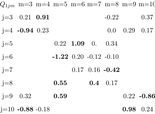
Generally speaking, the magnitudes of the quadratic coefficients Qnmp provide insight into the interactions between the different modes. Table III contains the values of the quadratic coefficients Qnm1 for 3≤n, m≤ 10. The dominant values which will be kept for the model are indicated in bold.
A. Simplified model
We first consider a simplified version of the model by making the following assumptions:
• we assume that the first two modesa1 and a2 are constant.
• we neglect quadratic terms of small magnitude.
• we model the energy transfer to the unresolved modes by assuming that their effect is to compensate for the production term i.e the interaction with the mean shear (mode 1). This means that
This leads to the following form for the model, which we will refer to as M0:
˙
a1 = 0 (10)
˙
a2 = 0 (11)
˙
a3 = 0.91a4 (12)
˙
a4 =−0.94a3 (13)
˙
a5 =−1.09a6+ 0.49a9 (14) ˙
a6 = 1.22a5 (15)
˙
a7 =−0.42a8 (16)
˙
a8 =−0.55a5+ 0.44a7 (17) ˙
a9 =−0.6a4−0.86a10 (18) ˙
a10 =−0.88a3+ 0.98a9 (19)
We can see that there are only interactions between modes with the same parity: (3,4,9,10) on the one hand and (5,6,7,8) on the other hand. The interactions between the normalized amplitudes (a2i−1, a2i),2 ≤ i ≤ 5 are of the form a2i−1 = −ωi(λλ2i2−1i )1/2a2i,
a2i =ωi(λ2λi−1
2i )
1/2a
2i−1, which correspond to propagative oscillatory solutions for the ampli-tudes √λnan, in agreement with the convective dynamics expected for the corresponding K´arm´an modes.
The averaged frequencies |ωi|= 2πfi identified for the pairs (3,4), (5,6), (7,8) and (9,10) are 0.92, 1.15, 0.43, 0.9, which correspond to frequencies (or Strouhal numbers) of 0.15, 0.18, 0.07 and 0.14. This is in good agreement with the main frequencies identified in the simulation. We emphasize that this prediction of the relevant time scales is based exclusively on the spatial structure of the modes, which are extracted from a set of samples arbitrarily separated in time. Since the computation is based on the derivatives of the spatial modes, some uncertainty exists in the determination of the time scales.
modes, even if the snapshots are obtained with large separations, which is evidence of the predictive abilities of the POD-based model.
B. Switches
We now examine if and how switches can be reproduced by a more complex version of the model, which we derive by relaxing the assumptions of the simplified model as follows:
• the second mode is allowed to vary.
• feedback is provided between the unresolved terms and the modes of the truncation.
As shown in [21], we assume that the rate of energy transferred to the small scales depends on the energy available in the largest scales. If more energy is available in the large scales, then more energy is extracted by the small scales and conversely. This leads to us to introduce a time-varying viscosity term, so that the effect of the unresolved terms is modelled as
Tn=Anan+n (20)
where
1. the time-averaged value < An> satisfies
< An>=−Ln−Qnn1, (21)
2. An contains a linear part and a quadratic part
An =< An>−αn
10
X
p=2
λp+αn
10
X
p=2
λp|ap|2, (22)
As has been shown in [21], we have
Tn= (< An >+αn N
X
p≥1
λp−αn N
X
p≥1
|ap|2)an+n (23)
where
αn=−
< An> 2PN
p≥2λp
.
of αi = α = 0.5 was used for all modes for the sake of simplicity. Examination of equation (20) and of the POD eigenvalues shows that about 50% of the turbulent viscosity is dependent on the amplitude of modea2. In that sense the structure of the model displays similarities with both [22] and [3]’s model, which includes a cubic term ina2. However it is derived from entirely different physical arguments.
3. n represents Gaussian noise. The amplitude of the noise used to integrate the model was determined using n ≈ |An|. We used 2 = 0.09 and i = 0.04 for 3 ≤ i ≤ 10. [A Gaussian variable was generated every 2.5 convective time units and linearly interpolated was used for the integration].
The modified model reads:
˙
a1 = 0 (24)
˙
a2 = (L2−α 10
X
2
a2pλp)a2 +2 (25)
˙
a3 = (L3−α 10
X
2
a2pλp)a2 + 0.71a4+3 (26)
˙
a4 = (L4−α 10
X
2
a2pλp)a2 −0.74a3+4 (27)
˙
a5 = (L5−α 10
X
2
a2pλp)a2 −1.09a6+5 (28)
˙
a6 = (L6−α 10
X
2
a2pλp)a2 −1.2a5+6 (29)
˙
a7 = (L7−α 10
X
2
a2pλp)a2 −0.42a8+7 (30)
˙
a8 = (L8−α 10
X
2
a2pλp)a2 −0.55a5+ 0.44a7+8 (31)
˙
a9 = (L9−α 10
X
2
a2pλp)a2 −0.6a4−0.86a10+9 (32)
˙
a10= (L10−α 10
X
2
a2pλp)a2−0.88a3+ 0.98a9 +10. (33)
The quadratic terms in the expression for a2 are not included in the model as their magnitude was small (we checked that including these terms in the equations did not change the dynamics reported below).
n 1 2 3 4 5 6 7 8 9 10
Li -0.05 -0.05 -0.05 -0.05 -0.05 -0.05 -0.05 -0.05 -0.05
< a2
n>M0 1 1 0.93 0.93 0.86 0.86 1.45 1.51 1.05 1.05
< a2n>M 1 1.05 0.29 0.29 0.18 0.18 1.01 1.03 2.05 2.33
TABLE II. Model linear coefficients and predicted energy
grow. Conversely, if mode a2 becomes too large, the energy transfer to the higher-order modes will be increased, which will in turn affect the energy of mode a2.
Figures 19 and 20 shows results of the model integration for a noise amplitude of about 0.15. Figure 19 (left) shows the 3-D coefficient a32d predicted with the model M along with the 2-D coefficient a2d
2 in the experiment, which appears a relevant comparison since, as shown in the previous section, there is a reasonably good correlation between a2 in 3-D and 2-D (0.6). The model displays time scales of O(1000) between switches, in agreement with experimental observations. Figure 19 (right) shows that the histogram of the amplitude is similar to that observed in the experiment in figure 6. This shows that the model is able to reproduce deviations in a way that is consistent with experiments. As figure 20 indicates, modes 3 to 10 are characterized by relatively fast oscillating time scales and slower amplitude variations. The frequencies of the amplitudes are shown in figure 20 (right) and compare relatively well with those measured in the simulation, given the crudeness of the truncation. Table II (last line) shows that the magnitude of the normalized POD amplitudes is relatively well estimated by the model with values of about 0.2 to 2 for the last modes of the truncation (we emphasize that the model contains only 20% of the total fluctuating energy). The main dynamics of the largest scales are therefore captured by the model.
VII. CONCLUSION
Q1jm m=3 m=4 m=5 m=6 m=7 m=8 m=9 m=10
j=3 0.21 0.91 -0.22 0.37
j=4 -0.94 0.23 0.0 0.29 0.17
j=5 0.22 1.09 0. 0.34
j=6 -1.22 0.20 -0.12 -0.10
j=7 0.17 0.16 -0.42
j=8 0.55 0.4 0.17
j=9 0.32 0.59 0.22 -0.86
[image:23.612.177.432.77.265.2]j=10 -0.88 -0.18 0.98 0.24
TABLE III. Quadratic interaction coefficients with the main mode Qj1m; Only coefficients larger
than 0.1 are indicated; only coefficients larger than 0.4 (indicated in bold) are included in the
model.
deviation, the effect of which is to gather flow streamlines around one of the base diagonals. 2-D POD analysis was performed in the near-wake in the simulation and compared with experimental results obtained for the same geometry. Despite the discrepancy in Reynolds number between the simulation and the experiment, an excellent agreement was observed for both the spatial structure and temporal statistics of the POD modes.
2-D results were then confronted with a 3-D approach. The energetic importance of the quasi-steady wake deviation was established. The evolution of this global 3-D deviation mode was relatively well captured by 2-D measurements in the near-wake. The next most energetic patterns are associated with vortex shedding and wake pumping. Characteristic frequencies were identified for each type of structure. Structures associated with wake pump-ing were characterized by a low frequency of about 0.08. Both symmetric and antisymmetric structures associated with vortex shedding in respectively the vertical and spanwise direc-tion were characterized by dominant frequencies of 0.19 and 0.23 in the far wake. A strong negative correlation was noted between the intensity of the vortex shedding modes and the magnitude of the quasi-steady deviation. In addition, increases in the base drag were found to correspond to an increase of the quasi-steady deviation, along with a shrinkage of the recirculation zone associated with wake pumping.
flow. The energy content of the modes was correctly captured by the model. A simplified model was able to single out the main frequencies of the POD amplitudes observed in the simulation from the spatial modes, regardless of the time separation between the snapshots used to compute POD. This predictive ability of the model is remarkable in view of the slow convergence of the decomposition, which reflects the complexity of the flow. A more elaborate version of the model was also considered. The approach is consistent with Rigas et al.’s model [22] and in particular the structure of the model would be the same if the POD truncation was limited to two modes. By accounting for the effect of the unresolved modes with a feedback term, the POD-based model was able to reproduce the characteristics of the switches in the wake deviation. The success of the model supports the idea that wake switching is triggered by higher-order modes.
[1] R.D. Brackston, J.M. Garci De La Cruz, A. Wynn, G. Rigas, and J.F. Morrison. Stochastic
modelling and feedback control of bistability in a turbulent bluff bodywake. J. Fluid Mech.,
802:726–749, 2016.
[2] O. Cadot. Stochastic fluid structure interaction of three-dimensional plates facing a uniform
flow. J. Fluid Mech., 794:726–749, 2016.
[3] O. Cadot, A. Evrard, and L. Pastur. Imperfect supercritical bifurcation in a three-dimensional
turbulent wake. Phys. Review E., 91(6), 2015.
[4] L. Dalla Longa, O. Evstafyeva, and A. S. Morgans. Simulations of the bi-modal wake past
three-dimensional blunt bluff bodies. Journal of Fluid Mechanics, 866:791809, 2019.
[5] A. Evrard, O. Cadot, V. Herbert, D. Ricot, R. Vigneron, and J. Delery. Fluid force and
symmetry breaking modes of a 3d bluff body with a base cavity. Journal of Fluids and
Structures, 61:99–114, 2016.
[6] O. Evsafyeva, A. Morgans, and L. Dalla Longa. Simulation and feedback control of the ahmed
body flow exhibiting symmetry breaking behaviour. J. Fluid Mech., 817, 2017.
[7] D. Fabre, F. Auguste, and J. Magnaudet. Bifurcations and symmetry breaking in the wake
of axisymmetric bodies. Phys. Fluids, 20(0517), 2017.
[8] M. Grandemange, O. Cadot, and M. Gohlke. Reflectional symmetry breaking of the separated
[9] M. Grandemange, M. Gohlke, and O. Cadot. Turbulent wake past a three-dimensional blunt
body. part 1 - experimental sensitivity analysis. J. Fluid Mech., 752:439–461, 2013.
[10] M. Grandemange, M. Gohlke, and O. Cadot. Turbulent wake past a three-dimensional blunt
body. part 1 - global modes and bi-stability. J. Fluid Mech., 722:1–26, 2013.
[11] P. Holmes, J.L. Lumley, and Gal Berkooz. Turbulence, Coherent Structures, Dynamical
Sys-tems and Symmetry. Cambridge University Press, 1996.
[12] M. Kiya and Y. Abe. Turbulent elliptic wakes. J. Fluids Struct., 13:1041–1067, 1999.
[13] R. Li, D. Barros, J. Bor´ee, O. Cadot, B.R. Noack, and L. Cordier. Feddback control of bimodal
wake dynamics. Exp Fluid, 51(4):158, 2016.
[14] J.M. Lucas, O. Cadot, V. Herbert, S. Parpais, and J. D´elery. A numerical investigation of the
asymmetric wake mode of a squareback ahmed body - effect of a base cavity. J. Fluid Mech.,
831:675–697, 2017.
[15] J.L. Lumley. The structure of inhomogeneous turbulent flows. In A.M Iaglom and V.I
Tatarski, editors, Atmospheric Turbulence and Radio Wave Propagation, pages 221–227.
Nauka, Moscow, 1967.
[16] R. Pasquetti and N. Peres. Simulation and feedback control of the ahmed body flow exhibiting
symmetry breaking behaviour. Computers and Fluids, 114:203–217, 2015.
[17] G. Pavia, M. Passmore, and C. Sardu. Evolution of the bi-stable wake of a square-back
automotive shape. Exp. in Fluids, 59:2742, 2018.
[18] A.K. Perry, G. Pavia, and M. Passmore. Influence of short rear end tapers on the wake of a
simplified square-back vehicle: wake topology and rear drag. Experiments in Fluids, 57(11),
2016.
[19] B. Podvin. A pod-based model for the wall layer of a turbulent channel flow. Phys. Fluids,
21(1):015111, 2009.
[20] B. Podvin and Y. Fraigneau. A few thoughts on proper orthogonal decomposition in
turbu-lence. Physics of FLuids, 29:020709, 2017.
[21] B. Podvin and A. Sergent. Precursor for wind reversal in a square rayleigh-b´enard cell. Phys.
Rev. E, 95:013112, 2017.
[22] G. Rigas, A.S Morgans, R.D. Brackston, and J.F. Morrison. Diffusive dynamics and stochastic
models of turbulent axisymmetric wakes. J. Fluid Mech., 778(R2), 2015.
axisymmetric bluff bodies. Fluid Mechanics and its Applications, 107:143–148, 2015.
[24] G. Rigas, A.R. Oxlade, A.S Morgans, and J.F. Morrison. Low-dimensional dynamics of a
turbulent axisymmetric wake. J. Fluid Mech., 755:159, 2014.
[25] P.J. Schmid. Dynamic mode decomposition of numerical and experimental data. J. Fluid
Mech., 656:5–28, 2010.
[26] L. Sirovich. Turbulence and the dynamics of coherent structures part i: Coherent structures.
Quart. Appl. Math., 45(3):561–571, 1987.
[27] E. Varon, Y. Eulalie, S. Edwige, P. Gilotte, and J.L. Aider. Chaotic dynamics of large-scale
structures in a turbulent wake. Phys. Review Fluids ., 2(034604), 2017.
[28] R. Volpe, P. Devinant, and A. Kourta. Experimental characterization of the unsteady natural
wake of the full-scale square back ahmed body: flow bi-stability and spectral analysis. Exp.
in Fluids, 56(5):1–22, 2015.
[29] E. Wassen, S. Eichinger, and F. Thiele. Simulation of active drag reduction for a square-back
vehicle. Notes on Numerical Fluid Mechanics and Multidisciplinary Design, 108:241–255,
mode u contour atz=−0.5 u contour aty=−0.4
n=3
n=4
n=5
n=6
n=7
n=8
n=9
[image:27.612.113.559.74.686.2]n=10
FIG. 14. Streamwise velocity contours of 3-D POD spatial modes 3 to 10 (from top to bottom);
FIG. 15. Left) amplitudes of the modesan, n=3, 5, 7, 9; right) power spectral density of the 3-D
POD mode amplitudes in the simulation |ˆan|2 - the red and black lines respectively correspond to
[image:28.612.131.552.76.243.2]the two frequencies 0.08 and 0.2.
FIG. 16. Left) energy of POD modes corresponding to quasi-steady deviation a22, spanwise (r2Kh=a23+a24) and vertical (r2Kv=a25+a26) vortex shedding intensities - vertical lines correspond
[image:28.612.87.542.406.630.2]FIG. 17. Left) base suction coefficient CB =−Cp obtained by integrating the pressure over the
rear of the body; right) correlation between the base suction coefficient and the POD amplitudes
FIG. 18. Power spectral density of the 3-D POD mode amplitudes 3 to 10|ˆa3D,M0
n |2in the simplified
model - the red and black lines respectively correspond to the two frequencies 0.08 and 0.2.
[image:30.612.121.520.483.624.2]FIG. 20. Left) amplitudes of 3-D POD amplitudes of modes 3, 5 , 7 and 9 in the model;
right) power spectral density of POD amplitudes in the model |aˆ3nd,M|2 - the red and black lines