Structural Dynamic Analysis and Model
Updating for a Welded Structure made from
Thin Steel Sheets
Thesis submitted in accordance with the requirements of
the University of Liverpool for the degree of Doctor in
Philosophy
by
Muhamad Norhisham Abdul Rani
To my dear mother , father and sister
Abstract
Modern large, complex, engineering structures normally encompass a number of substructures which are assembled together by several types of joints. Despite, the highly sophisticated finite element method that is widely used to predict dynamic behaviour of assembled complete structures, the predicted results achieved, of assembled structures are often far from the experimental observation in comparison with those of substructures. The inaccuracy of prediction is believed to be largely due to invalid assumptions about the input data on the initial finite element models, particularly those on joints, boundary conditions and also loads. Therefore, model updating methods are usually used to improve the initial finite element models by using the experimentally observed results.
This thesis is concerned with the application of model updating methods to a welded structure that consists of several substructures made from thin steel sheets that are assembled together by a number of spot welds. However, the welded structure with a large surface area is susceptible to initial curvature due to its low flexible stiffness or manufacturing or assembling errors and to initial stress due to fabrication, assembly and welding process of substructures. Nevertheless, such initial stress is very difficult to estimate by theoretical analysis or to measure. This thesis puts forward the idea of including initial curvature and/or initial stress (which have a large effect on natural frequencies) as an updating parameter for improving the performance of the finite element model of a structure made from thin steel sheets.
where the confidential and proprietary issues of modelling work are of concern between the collaborating companies, in which the finite element models of the substructures could not be revealed and only the condensed matrices of the substructures are used instead, the areas of the substructures having fewer number of interface nodes would always be the first choice as the interface nodes. For welded structures, the nodes in the vicinity of spot weld element models are few and hence are usually taken as the interface nodes for connecting substructures. However, the present MSC. NASTRAN superelement model reduction procedures are known not to allow the nodes of CWELD elements to be the interface nodes of substructure.
Prior to the present study, no work appears to have been done to use the nodes of CWELD elements as the interface nodes of substructures in the investigation of dynamic behaviour of welded structures. In this work, the application of branch elements as the interface elements of substructure are proposed and tested. Prior to the present study, it also appears that there has been no work done concerning the adjustment of the finite element model of the welded structure by including the effects of initial curvatures, initial stress and boundary conditions that are contributing to the modelling errors, via the combination between the Craig-Bampton CMS and model updating.
Acknowledgements
With this opportunity, I would like to extend my gratitude and appreciation to my dearest supervisor Prof. Huajiang Ouyang who I knew two years before I decided to pursue my PhD. During that period I often emailed to him seeking his expertise in the issues of structural dynamics. His highly responsive attitude to every question that I emailed and his intellectual approaches to the issues I brought forward were the chief reasons that I decided on doing a PhD under his supervision. On top of that, I would like to record my sincerest thankfulness to him for his many helpful suggestions, excellent discussions, supervision and also encouragement throughout this research. I also would like to thank my second supervisor Dr. T. Shenton for his helpful inputs and generosity in his time.
I would like to acknowledge Prof. John E. Mottershead for his work on model updating, his valuable textbook and papers have become very good resources, not only for my research but for other scientific and engineering communities. I also would like to thank him for his willingness to lend me all his paper references and to take a photo with me for the sake of my Malaysian friends.
I owe a debt of gratitude to Dr. Simon James for his expertise and invaluable advice in ensuring my experimental work was successfully carried out. I would also like to express my appreciation to Mr. Tommy Evans from the Core Services Department for his readiness to fabricate the weld structure and his special attention to my project. This research would not have been completed without their great support.
Special appreciation to Mr. Ir. John, Dr. Dan. Stancioiu, Dr. Huaxia Deng and Dr. Ruiqiang for their valuable advice and great suggestions and with whom I have always been working, having coffee and generally hanging out together.
In addition, thank you to the following people: Mr. M.S. Mohd Sani, Dr. Weizhuo Wang, Ms. N. Hassan, Mr. M. Y. Harmin, Mr. A. S. Omar and Mr. R. Samin who have aided me in my research and through difficult times; and to K. Zhang and Q. Ouyang who have often spent time together with me having coffee and discussing the technical and global economic issues.
I am also grateful to my dearest sister Ms. Norhayati who has always cheered me up in times of trouble and to my best friends Dr. Bob Kana, Mr. Herry Yunus, Mr. Syaiful and Mr David Paul Starbuck for their kindness , great continuous support and encouragement.
Lastly, it would not have been possible for me to complete my research without the outstanding moral support from my loving parents, my dearest wife Azurina Hj Zainal Ratin and son, Umar Haziq. My future son Mansor Haziq and daughter Sarah Haziq are certainly not to be omitted from my acknowledgements.
Table of Contents
Abstract ... iii
Acknowledgements ... v
Content ... vii
List of Figures ... xi
List of Tables ... xv
List of Symbols and Abbreviations ... xxi
Chapter 1 - Introduction ... 1
1.1 Introduction ... 1
1.1.1 Superelement ... 3
1.1.2 Residual structure ... 3
1.1.3 Boundary nodes ... 3
1.1.4 Bending moment of inertia ratio (12I/T3) ... 3
1.1.5 Interior nodes ... 4
1.1.6 CEFE ... 4
1.1.7 Branch elements ... 4
1.1.8 SEMU ... 4
1.2 Research goal and objectives ... 5
1.3 Research scope ... 6
1.4 List of publications ... 7
1.5 Thesis outline ... 7
Chapter 2 - Literature Review ... 11
2.1 Introduction ... 11
2.2 Structural modelling ... 13
2.3 Finite element model updating ... 15
2.3.1 Direct methods of finite element model updating ... 18
2.4 Structural joint modelling ... 21
2.4.1 Bolted joint modelling ... 22
2.4.2 Welded joint modelling ... 24
2.5 Dynamic substructuring and component mode synthesis ... 37
2.6 Conclusions ... 44
Chapter 3 - Experimental Modal Analysis of the Substructures and the Welded Structure ... 47
3.1 Introduction ... 47
3.2 Experimental modal analysis ... 48
3.2.1 Introduction ... 48
3.2.2 Basics of experimental modal analysis ... 48
3.2.3 Modal testing ... 49
3.2.4 Force and vibration transducers ... 52
3.2.5 Acquisition and analysis systems ... 53
3.2.6 Method of support ... 53
3.2.7 Method of excitation ... 54
3.2.8 Measuring points (degrees of freedom) ... 57
3.3 Modal test of the substructures of the welded structure ... 58
3.3.1 Thin steel sheets ... 60
3.3.2 Modal test of side wall 1 and side wall 2 ... 61
3.3.3 Modal test of stopper 1 and stopper 2 ... 65
3.3.4 Modal test of the bent floor ... 69
3.4 Modal test of the welded structure ... 73
3.5 Conclusions ... 78
Chapter 4 - FE Modelling and Model Updating of Substructures ... 89
4.1 Introduction ... 89
4.1.1 FE method and model updating ... 91
4.1.2 FE model updating ... 94
4.1.3 Iterative methods of FE model updating ... 96
4.1.4 FE model updating via MSC NASTRAN (SOL200) ... 96
4.3 FE modelling and model updating of the substructures ... 99
4.3.1 FE modelling and model updating of side wall 1 and side wall 2 ... 99
4.3.2 FE modelling and model updating of stopper 1 and stopper 2 ... 112
4.3.3 FE modelling and model updating of the bent floor ... 122
4.4 Conclusions ... 132
Chapter 5 - FE Modelling and Model Updating of the Welded Structure ... 133
5.1 Introduction ... 133
5.2 FE modelling of the welded structure ... 135
5.2.1 CWELD elements ALIGN format (CEAF) ... 137
5.2.2 CWELD elements ELPAT format (CEEF) ... 139
5.2.3 Results and discussion of CEAF and CEEF ... 141
5.3 FE model updating of the welded structure ... 141
5.4 FE model updating of the welded structure considering initial stress and the effect of boundary conditions ... 150
5.5 Conclusions ... 162
Chapter 6 - Substructuring Scheme based Model Updating ... 163
6.1 Introduction ... 163
6.2 Component mode synthesis (CMS) ... 165
6.3 CMS-Fixed boundary method based substructures ... 167
6.4 Description of the superelements and analysis ... 186
6.5 Results and discussion of the superelements ... 192
Chapter 7 - Conclusions and Future Work ... 211
7.1 Introduction ... 211
7.2 Main contributions of this thesis ... 212
7.3 Experimental modal analysis ... 213
7.4 Substructure modelling and model updating ... 214
7.5 Welded structure modelling and model updating ... 215
7.6 The Craig-Bampton CMS based model updating ... 216
7.7 Suggestions for future work ... 218
Appendix A ... 221
Appendix B ... 223
List of Figures
Chapter
2
2
.1 Illustration of resistance spot welding process ... 252
.2 Unique grid point normal for adjacent shell elements ... 292.3 The size of mesh for CWELD element ... 34
Chapter
3
3.1 Typical modal analysis test ... 513.2 Accelerometer (Kristler 8728A) ... 52
3.3 Schematic diagram of shaker excitation test set up ... 55
3.4 Schematic diagram of hammer excitation test set up ... 55
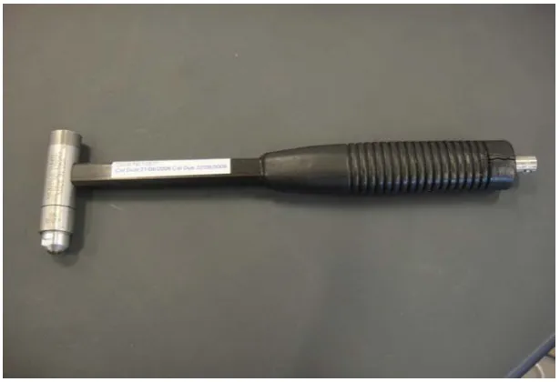
3.5 PCB impact hammer ... 56
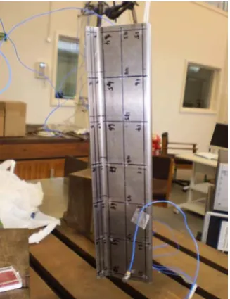
3.6 The welded structure ... 58
3.7 A truncated body-in-white ... 59
3.8 Schematic diagram of the side wall test set up ... 61
3.9 Side wall 1 and side wall 2 test set up ... 63
3.10 Schematic diagram of the stopper test set up ... 66
3.11 Stopper 1 test set up ... 67
3.12 Stopper 2 test set up ... 67
3.13 Schematic diagram of the bent floor test set up ... 69
3.14 Bent floor test set up ... 70
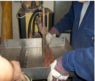
3.15 Spot welding process ... 74
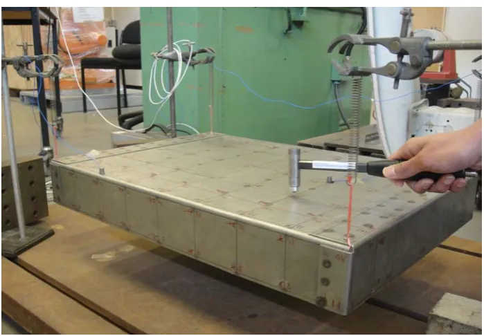
3.16 Schematic diagram of the welded structure test set up ... 75
3.17 The test set up of the welded structure ... 75
3.18 1st, 2nd and 3rd pair of measured modes of side wall 1 ... 79
3.19 4th and 5th pair of measured modes of the side wall 1 ... 80
3.20 1st, 2nd and 3rd pair of measured modes of the side wall 2 ... 81
3.21 4th and 5th pair of measured modes of the side wall 2 ... 82
3.22 1st, 2nd and 3rd measured modes of the stopper 1 ... 83
3.23 1st, 2nd and 3rd measured modes of the stopper 2 ... 84
3.25 4th and 5th pair of measured modes of the bent floor ... 86
3.26 1st, 2nd and 3rd pair of measured modes of the welded structure .... 87
3.27 4th and 5th pair of measured modes of the welded structure ... 88
Chapter 4
4.1 FRFs of the substructure (a) and the welded structure (b) ... 924.2 Visual models of side wall 1 (SW1) and side wall 2 (SW2) ... 100
4.3 The convergence of the updating parameter of side wall 1 ... 100
4.4 The convergence of the updating parameter of side wall 2 ... 102
4.5 1st, 2nd, 3rd, 4th and 5th pair of experimental (EXP) and updated FE modes of side wall 1 (SW1) and side wall 2 (SW2) ... 110
4.6 6th, 7th, 8th, 9th and 10th pair of experimental (EXP) and updated FE modes of side wall 1 (SW1) and side wall 2 (SW2) ... 111
4.7 Visual models of stopper 1 (S1) and stopper (S2) ... 112
4.8 Backbone of stopper 1 and stopper 2 ... 115
4.9 The convergence of the updating parameter of stopper 1 ... 117
4.10 The convergence of the updating parameter of stopper 2 ... 118
4.11 1st, 2nd and 3rd pair of the experimental (EXP) and the 2nd updated FE modes of stopper 1 (S1) and stopper 2 (S2) ... 121
4.12 Visual models of the bent floor ... 123
4.13 FE modelling of the bent floor considering the effect of boundary conditions ... 126
4.14 The convergence of the updating parameters of the bent floor .... 129
Chapter 5
5.1 Visual models of the welded structure ... 136
5.2 Point to point connection defined with ALIGN format ... 137
5.3 Patch to patch connection defined with ELPAT format ... 139
5.4 The results of sensitivity analysis of CWELD properties ... 143
5.5 The measurement of the diameter of physical spot weld ... 145
5.6 FE model of patches from the truncated FE model of the Welded structure ... 146
5.7 The results of sensitivity analysis of CWELD properties and the Young’smodulus of patches ... 147
5.8 The results of sensitivity analysis of CWELD properties, the Young’s modulus of patches and the boundary conditions (BC) ... 148
5.9 Characterization of initial stress on the FE model of the welded structure ... 154
5.10 The results of sensitivity analysis of CWELD properties and the Young’smodulus of patches and the boundary conditions (BC) ... 155
5.11 The convergence of the updating parameters of the 5th updated FE model of the welded structure ... 159
5.12 1st, 2nd, 3rd, 4th and 5th pair of mode shapes of the welded structure calculatedfrom experiment (EXP), initial FE model (IFEM) and updated FE model (UFEM) ... 160
Chapter
6
6.1 Schematic diagram of substructuring process ... 167
6.2 Schematic diagram of reduced model ... 170
6.3 CWELD element connecting to branch elements (patches) ... 183
6.4 Superelement models of the welded structure ... 186
6.5 Residual structure and branch element sets ... 189
6.6 Superelement of side wall and branch element leftover ... 190
6.7 Superelement of stopper and branch element leftover ... 191
6.8 The combination of analysis results of the augmentation effect .. 195
6.9 The convergence of the updating parameters of case study 3 ... 204
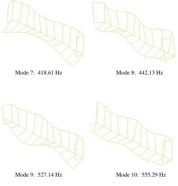
6.10 1st, 2nd, 3rd, 4th and 5th triplets of mode shapes of welded structure calculated from experiment (EXP), full FE model (FFEM) and SEMU ... 207
List of Tables
Chapter
3
3.1 Nominal values of mild steel material properties of side wall 1 and side wall 2 ... 60
3.2 Number of measuring points and measuring directions of side wall 1 and side wall 2 ... 64
3.3 Experimental and numerical frequencies of side wall 1 and side
wall 2 ... 65
3.4 Number of measuring points and measuring directions of stopper 1 and stopper 2 ... 68
3.5 Experimental and numerical frequencies of stopper 1 and
stopper wall 2 ... 68 3.6 Experimental and numerical frequencies of the bent floor ... 71 3.7 Number of measuring points and measuring directions of the bent
floor ... 72
3.8 Number of measuring points and measuring directions of the welded structure ... 76
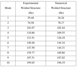
3.9 Experimental and numerical frequencies of the welded structure . 77
Chapter 4
4.1 Nominal values of mild steel material properties of side wall 1 and side wall 2 ... 101 4.2 Comparison of results between the tested and initial FE model of
side wall 1 ... 102 4.3 Comparison of results between the tested and initial FE model of
the side wall 2 ... 102 4.4 Summarised results of the sensitivity analysis of side wall1 and
4.5 Three comparisons of results between the tested and FE models of side wall 1 ... 104 4.6 Updated value of parameter of side wall 1 ... 105 4.7 Three comparisons of results between the tested and FE models
of side wall 2 ... 106 4.8 Updated value of parameter of side wall 2 ... 106 4.9 The comparisons of results calculated from different number of measured frequencies (NoMF) of side wall 1 - 1st to 5th ... 108
4.10 The comparisons of results calculated from different number of measured frequencies (NoMF) of side wall 1 - 6th to 10th ... 108
4.11 The comparisons of results calculated from different number of measured frequencies (NoMF) of side wall 2 - 1st to 5th ... 109
4.12 The comparisons of results calculated from different number of measured frequencies (NoMF) of side wall 2 - 6th to 10th ... 109
4.13 Comparison of results between the tested and initial FE model of
stopper 1 ... 113 4.14 Comparison of results between the tested and initial FE model of
stopper 2 ... 113 4.15 Comparison of results between the tested and 1st updated FE
model of stopper 1 ... 114 4.16 Comparison of results between the tested and 1st updated FE
model of stopper 2 ... 114 4.17 The details of the two different collectors of the FE models of
stopper 1 and stopper 2 ... 116 4.18 The FE results of stopper 1 and stopper 2 due to the change in the
backbone thickness (BT) ... 116 4.19 The updated value of the updating parameter of stopper 1 ... 117
4.20 The updated value of the updating parameter of stopper 2 ... 118 4.21 Three comparisons of results between the tested and FE models
of stopper 1 ... 119 4.22 Three comparisons of results between the tested and FE models
4.23 The comparisons of results calculated from different number of measured frequencies (NoMF) of stopper 1 - 1st to 3rd ... 120 4.24 The comparisons of results calculated from different number of
measured frequencies (NoMF) of stopper 2 - 1st to 3rd ... 120 4.25 Comparison of results between the tested and initial FE model of the bent floor ... 124
4.26 Comparison of results between the tested and updated Young's modulus (UYM) based FE model of the bent floor ... 125 4.27 The updated value of the updating parameter of the bent floor ... 125 4.28 Summarised results of the sensitivity analysis of the bent floor .. 127 4.29 Three comparisons of results between the tested, the initial FE and theupdated Young’s modulus and PELAS (UYMP) based FE
model of the bent floor ... 128 4.30 The updated values of the updating parameters of the bent floor 128 4.31 The comparisons of results calculated from different number of
measured frequencies (NoMF) of bent floor - 2nd to 5th ... 130 4.32 The comparisons of results calculated from different number of
measured frequencies (NoMF) of bent floor - 6th to 10th ... 130
Chapter 5
5.1 Comparison of results between the tested and the CEAF FE
model of thewelded structure ... 138 5.2 Comparison of results between the tested and the CEEF FE
model of thewelded structure ... 140 5.3 Summarized results of the sensitivity analysis of the welded
structure using the updating parameters of the CWELD element properties ... 142
5.5 Updated value of parameter of CWELD diameter ... 145 5.6 Updated values of parameter of the 2nd updated FE model of the
welded structure ... 146 5.7 Comparison of results between the tested and the 2nd updated FE
model of the welded structure ... 147 5.8 Comparison of results between the tested and the 3rd updated FE
model of the welded structure ... 149 5.9 Updated values of the updating parameters of the 3rd updated FE
model of the welded structure ... 150 5.10 Comparison of results between the tested and the 4th updated FE
model of the welded structure ... 156 5.11 Updated values of the updating parameters of the 4th updated FE
model of the welded structure ... 156 5. 12 Comparison of results between the tested and the 5th updated FE
model of the welded structure ... 157 5.13 Updated values of the updating parameters of the 5th updated FE
model of the welded structure ... 159
Chapter 6
6.1 Description of superelement and residual structure ... 186 6.2 The set up of the superelements for case study 1 ... 194 6.3 Percentage frequency error between the superelement model and the full FE model ... 197
6.4 The set up of the superelement model updating for case studies 2 and 3 ... 199
6.5 The results of case study 2 for the full FE and superelement model
updating ... 200 6.6 The results of case study 3 for the full FE and superelement model
6.8 The comparisons of results calculated from different number of measured frequencies (NoMF) of SEMU - 2nd to 5th ... 206 6.9 The comparisons of results calculated from different number of
List of Symbols and Abbreviations
E Young's modulus
G shear modulus
mass density
Poisson's ratio
frequency in rad/sec
FE i
th
i numerical eigenvalue
EXP i
th
i experimental eigenvalue
Zm vector of measured data involving eigenvalues or eigenvectors Zj vector of analytical response
vector of structural updating parameters
S eigenfrequency sensitivities
M mass matrix
C damping matrix
K stiffness matrix
f t vector of applied forces
q vector of displacements
q vector of velocities
q
vector of accelerations
vector of eigenvectors
MS th
S substructure’s mass matrix vector
KS Sth substructure’s stiffness matrix vector XS Sth substructure’s displacement matrix vector FS Sth substructure’s force vector
ˆ
MSBB reduced mass matrix ˆ
KSBB reduced stiffness matrix
B constraint modes or boundary node functions
F inertia-relief modes
B boundary degrees of freedom
I interior degrees of freedom
r rigid body
BC boundary conditions
CEAF CWELD element ALIGN format CEEF CWELD element ELPAT format CMS component mode synthesis CWELD weld element connection EMA experimental modal analysis
EXP experimental
FE finite element
FFEM full finite element model IFEM initial finite element model MAC modal assurance criteria NGV natural gas vehicle
NoMF number of measured frequencies NVH noise vibration and harshness PELAS scalar elastic property
RSW resistance spot weld
S1 stopper 1
S2 stopper 2
SEMU substructuring or superelement based model updating SW1 side wall 1
SW2 side wall 2
UFEM updated finite element model UYM updated Young's modulus
Chapter 1
Introduction
1.1 Introduction
Structural dynamic analyses continue to present a major concern for a very wide range of engineering products today. This concern has constantly demanded and challenged engineers who need efficient and practical methods for accurately predicting and investigating structural dynamic problems. Numerical methods have become preferable and extremely powerful for understanding the dynamic characteristics of structures in comparison with the experimental modal analysis in which the number of testing scenarios are limited.
The ability to investigate the dynamic characteristics of structures numerically allows structures to be designed economically and competitively. However, the accomplishment must not be at the expense of safety, reliability and durability which highly depend on the dynamic characteristics of structures. Numerical models, particularly the finite element models, are, in fact, constructed based on assumptions about the model and material properties of structures. The best way to develop confidence in the numerical models is to compare its predicted results with measured results on actual hardware. The discrepancies between the numerical results and experimental results drive a process in which the numerical models are systematically adjusted to become a closer representation of the tested structures. The chief expectation from the systematic adjustment process is a better reconciliation between both models.
difficulties in obtaining a satisfactory level of accuracy of the results are the complexity of joint types, the uncertainties in boundary conditions, the presence of initial stress and also the inaccurate description of the interactions between substructures.
The configuration of structures as described in the preceding paragraph, for example a car body-in-white is an assembly of a number of substructures which are formed from many components. The components are made from thin metal sheets and are assembled together by thousands of joints. Resistance spot weld (RSW) is one of the joint types that are widely used in automotive engineering. As the paramount contributors of a car’s dynamic characteristics, spot welds are highly required to be properly modelled. However because many automotive components are designed and analysed in parallel, different CAE engineer teams supply components with dissimilar meshes. This has lead to a difficulty in modelling the spot welds which is cumbersome, time-consuming and error prone. As a result, the confidence in the correlation between the numerical and experimental results of the global assembled structures is questionable.
In this work, several unfamiliar technical and non-technical terms have been used
for describing certain modelling scenarios. The following items account for the
definition of:
1.1.1 Superelement
Superelement is a combination of several particular regular finite elements into a
single unit form of element in which part of the degrees of freedom is condensed
out for computational and modelling purposes. Superelement and substructure are
interchangeable terms in this work.
1.1.2 Residual structure
Residual structure is, by definition, the substructure in which the condensation of matrices is not performed. It is the substructure in which the condensed matrices of superelements are combined and solved. The substructure which is totally represented in physical coordinates. Furthermore the residual structure is also the substructure in which the design space such as model updating and optimization process are carried out.
1.1.3 Boundary nodes
Boundary nodes are the interchangeable term for interface nodes. They are best
described as those that are retained for further analysis and those to which the
matrices of superelements are reduced and also those that connect a superelement
with another superelement or a residual structure.
1.1.4 Bending moment of inertia ratio (12I / T3)
Bending moment of inertia ratio is the ratio of the actual bending moment inertia of the shell element, I , to the bending moment of inertia of a homogeneous shell
element, T 3/12. MSC NASTRAN is a unit less code, however, if SI system of units is used then 12I T/ 3 would have the units of meters. The I is the second moment of area of the cross section of the shell, which is by definition rectangular
if the thickness at all GRID points is the same. T is the thickness of the shell and
has units of meters. The default value of 12I / T3 is 1.0 for a homogeneous shell
312
/
I = WT
Where:
W = section width (the width of the element)
T = section height ( the thickness of the element)
The unit of 12I / T3is meter.
1.1.5 Interior nodes
The nodes that can be thought of as those that are condensed out during the
superelement processing. All nodes that are not boundary nodes can be regarded as
interior nodes.
1.1.6 CEEF
It stands for CWELD elements in ELPAT format. This is the format that is used to
represent the eighty spot welds on the welded structure after CWELD elements in
ALIGN format have failed to demonstrate good predictive models for the spot
welds.
1.1.7 Branch elements
Branch elements, in context of this work, are a group of elements surrounding CWELD elements in ELPAT format (CEEF). Using ELPAT format, additional support nodes are automatically generated and evenly positioned on different
elements, up to 3x3. The surrounding elements namely branch elements may be
included into the modelling spot weld, instead of only one element.
1.1.8 SEMU
Superelement based model updating or SEMU is a combination of two methods
between superelement and model updating. It is an efficient method for
substructuring and model updating for large, complex structures in which spot
welds are used to join their substructures. SEMU is chiefly constructed and used
for efficiently assisting in the development of reliable predictive models of
structures, in particular involving very large complex structures and also spot
1.2 Research goal and objectives
The chief goal of this research is to present an efficient method for the identification and reconciliation of the dynamic characteristics of finite element model. The proposed method is effectively valuable for large, complex structures in which spot welds are the joint interfaces. Four objectives are identified and they are:
1. To perform finite element modelling and modal testing on a structure which is an assembly of substructures made from thin metal sheets and joined by a number of spot welds
2. To perform model updating of the above-mentioned welded structure in order to improve the accuracy of finite element model.
3. To construct and apply superelement based model updating to the welded structure
4. To validate the accuracy and efficiency of superelement based model updating
Performing modal testing on the tested substructures and welded structure
Performing comparative study for identifying the most
reliable CWELD elements in modelling physical spot welds Performing normal modes analysis on finite element models
of substructures and welded structure
Performing sensitivity analysis for identifying the most potential updating parameters
Performing model updating on the full finite element models
of substructures and welded structure
Performing superelement based model updating on welded
structure
Performing comparison of finite element derived modal
1.3 Research scope
The scope of this research includes the following steps:
1. Finite element modelling and modal testing are performed on substructures and the welded structure. The first ten modes are investigated numerically and experimentally.
2. Model updating is divided into two phases. The first phase is performed on finite element models of substructures. The Young Modulus, thickness and boundary conditions are among the updating parameters used. The second phase is carried out on finite element model of the welded structure in which a parameter (bending moment of inertia ratio), CWELD elements and boundary conditions are used as the updating parameters. In this work, updating boundary conditions refer to updating the properties of NASTRAN CELAS elements used to represent the four sets of suspension springs and nylon strings to approximate free-free boundary conditions of the modal tests of the bent floor and the welded structure (see Figure 3.14 page 70 and Figure 3.17 page 75).
3. Construction of superelement based model updating is based on the Craig-Bampton fixed interface methods and the application of NASTRAN Optimizer SOL 200 and also of specially designed branch elements. While application of superelement based model updating is to show the efficiency of the method in the reconciliation of the finite element model with the tested structure and also to assist effectively in the development of a reliable predictive model for structural dynamic investigations.
1.4 List of publications
ABDUL RANI, M. N. A., STANCIOIU, D., YUNUS, M. A., OUYANG, H., DENG, H. & JAMES, S. 2011. Model Updating for a Welded Structure Made from Thin Steel Sheets. Applied Mechanics and Materials, vol. 70, pg. 117-122.
YUNUS, M. A., RANI, M. N. A., OUYANG, H., DENG, H. & JAMES, S. 2011. Identification of damaged spot welds in a complicated joined
structure. Journal of Physics: Conference Series, vol. 305, no.1, pg. 1-10.
1.5 Thesis outline
This thesis consists of seven chapters covering introduction, literature review, experimental modal analysis of structure, finite element modelling and model updating of the substructures, finite element modelling and model updating of the welded structure, substructuring method based model updating of the welded structure, conclusions and future work.
Chapter 1 gives an overview of the introduction, the goal, objectives and scope of research.
Chapter 2 reviews previous work in the field of finite model updating, substructuring modelling schemes, superelement model updating, modelling spot welds, model updating of spot welds and also the effect of initial curvatures and initial stress towards the accuracy of natural frequencies.
Chapter 3 covers comprehensive experimental modal analyses of substructures and the welded structure in which experimentally derived results, natural frequencies in particular are used for updating the finite element models. These include addressing the problems encountered in characterising the natural frequencies and modes shapes of substructures and of the welded structure and also highlighting several important factors in ensuring the accuracy of the results calculated such as the number of measuring points and accelerometers, the weight
of accelerometers, method of support and method of excitation have been briefly
Chapter 4 presents the finite element modelling and model updating procedures. These include elaborating the formulation used in finite element method, model updating and the description of Design Sensitivity and Optimization SOL200 provided in NASTRAN. This chapter also covers the development of finite element models of the substructures through which model updating methods are performed to minimise the errors introduced in the finite element models. Iidentifying the source of discrepancies is the most challenging aspect of the updating process. This chapter reveals that the inclusion of the PELAS as one of the updating parameters could result in a dramatic reduction in the first frequencies of the bent floor. This chapter also discusses that the consideration of the thickness reduction in the backbone leading to more representative models of the stoppers for model updating process.
Chapter 5 discusses the work of finite element modelling and model updating of the welded structure. The construction of the finite element model of the welded structure is based on the updated finite element models of the substructures (structural components). This chapter also discusses how the combination between the sensitivity analysis, the inputs of the technical observation and engineering judgment has proved to be a powerful tool for localizing the main sources of the errors which are the boundary conditions and initial stress. The combination has led to the significant reduction in the discrepancies, dropping from 26.44 to 7.30 percent in total error, between measured and predicted frequencies. The outstanding capability of CWELD elements in ELPAT format over ALIGN format in representing spot welds is elaborated and demonstrated in this chapter. Another significant finding in this chapter is that a methodology which is using bending moment of inertia ratio is proposed for model updating in the presence of initial stress and initial curvatures on the structure.
substructure or a residual structure, a process which gives modal solution for the structure. This chapter also stresses that the use of normal procedure for assembling superelements together via the nodes of CWELD elements in ELPAT format as the boundary nodes fails in arriving at a satisfactory solution. On top of that this chapter reveals that SEMU has been successfully used for the reconciliation of the finite element model with the tested structure of the welded structure and stresses the use of branch elements, the efficient settings and the augmentation (using residual vectors) in SEMU is of the essence of the success. Another outstanding findings in this chapter is that SEMU has proven capability of accurately minimizing the uncertainties in the finite element model in comparison with the full finite element model and SEMU has also shown better efficiency in dealing with the analysis involving a large number of iterations.
Chapter 2
Literature Review
2.1 Introduction
The efficient methods for the numerical prediction of dynamic characteristics of large, complex structures have been the subject of much investigation in the scientist and engineer communities. The finite element method has become the predominant method for numerically predicting structural behavior and the results obtained are very useful for virtual product development. Nonetheless, constructing accurate finite element models for modern structures which are usually large and complex is not an easy task (Friswell and Mottershead, 1995). This is because the sort of structures requires a very large number of degrees of freedom to be accurately modeled and the accuracy of the methods improves as more elements are used (Cook, 1989).
For the predicted results of finite element models to correlate as closely as possible with the measured results, systematic adjustments must be made to minimise the errors introduced to the models. The finite element model updating method has become the accepted method for the reconciliation. Structural model updating methods ( Mottershead and Friswell, 1993) have been proposed to reconcile the finite element results with the measured results. There are many different methods of model updating, and the most predominant one is the iterative method so is the direct method.
The method has the advantage of allowing the updating parameters of finite element models to be updated during the reconciling process at every iteration. However, the optimisation algorithm (which is a gradient based method) used in the model updating in this project requires repeated computations of the finite element models. Using these conventional methods, the number of reanalyses during the solution process may be reduced but it is necessary to calculate repeatedly the response derivatives or the sensitivity coefficients. Therefore, when these conventional methods are applied to a modern engineering structure which is in the form of an assembly of several large substructures that consists of a very large number of components, with many unknowns, obviously, these methods are often perceived to be inefficient and computationally burdensome.
The substructuring schemes are obviously outstanding in a situation in which optimisation is merely required for a particular substructure. This distinct advantage is clearly seen when modifications are only performed on the particular substructure. Only the system matrices of the affected substructure are to be reanalysed while other substructures' system matrices remain intact ( Perera and Ruiz, 2008). This leads to tremendous reduction in the expenditure of computational time in comparison with the conversional method of optimization in which full finite element models are used.
In this chapter, previous works in the domains of structural modelling, finite element model updating methods, structural joint modelling and substructuring schemes are reviewed and discussed especially those associated with the most popular methods for model updating, substructuring and spot weld modelling. At the end of this chapter the type of model updating, spot weld modelling and substructuring that have been studied in this work are drawn with concise conclusions.
2.2 Structural modelling
An approximate approach involving discretisation of structures into a potentially large number of elements, whose behaviour is known, came to prominence in the late fifties (Kamal et al., 1985). The approach which is so called the finite element method (FEM) allows the stiffness and mass distribution of a structure to be described in matrix terms with rows and columns representing the active degrees of freedom. The term finite element was firstly used by Clough (1960) in 1960. The finite element method has become the predominant method of analysing structural performance. However, this method offers many choices that require engineers to make the decision in the construction of finite element models.
The estimation of the properties of material and geometric performed by engineers usually has a high tendency towards the use of textbook values and the initial design rather than the measured data. As such, therefore, the predictions of structural performance based on the finite element models are not flawless. In fact Maguire (1995) discovered that large variations in the predicted results of structural dynamic behaviour obtained from a number of finite element models of the same structure constructed by different engineers. The same issue of the inaccuracy of the predictions was elaborated by Ewins and Imregun (1986). Actually there are several factors that can be identified as being responsible for the inaccuracy of predictions in structural dynamic behaviour. These principally include:
mis-estimation of structural material properties inaccurate modelling of structural geometry
inaccurate modelling boundary conditions and loads poor choice of element type and quantity required
difficulty in modelling complex structural systems, the most common and
widespread being the pitfalls in the modelling of structural joints
2.3 Finite element model updating
The elimination of some errors in the finite element models seems to be impossible even though well rounded selection of data including the use of practical and measured parameters in the process of constructing the finite element models is used. For the success of construction of reliable finite element models, comparative evaluation of both the predicted results and measured results is vital because the results of the comparison provides some insights into the likely sources of errors in the finite element models. The requirement to improve the finite element models derived results with respect to those obtained from the tested models is a part of the model correlation process. There are many techniques that have been developed through which the finite element models of structures are adjusted by varying the parameters of numerical models to fit the experimentally measured data.
In an era dominated by high technology, demands on the accuracy in predicting structural dynamic performance of large and complex structures, in particular in automotive and aerospace industry for safety and economic benefits, are surging. With increasing size and complexity of the structures involved, as a result, model updating has become more difficult to efficiently perform. Therefore systematic and efficient approaches are necessary. In the past few decades, vigorous effort has been made in order to improve the correlation between analytical model of structures and measured data through the application of modal data. One of the earliest attempts was published by Rodden (1967) who identified the structural influence coefficients via the application of measured natural frequencies and mode shapes of an effectively free-free ground vibration test. While Berman and Flannelly (1971) were among the first authors who presented a systematic approach through which the improvement of stiffness and mass characteristics of a finite element model was performed. The improvement was only achieved through the mass matrix, but not through the stiffness matrix because in this case it did not resemble a true stiffness matrix.
The initiation of the development of model updating algorithms began in the 1970s as a results of increasing reliability and confidence in measurement technology. The iterative methods through which analytical models can be reconciled with measured data have become of interest to researchers since. Collins et al. (1974) formulated and demonstrated a method for the statistical identification of a structure. Through the proposed method they maintained the specific finite element character of the model and used values of the structural properties originally assigned to model by the engineer as the starting point. The original property values were modified to make the model characteristics conform to the experimental data.
Chen and Garba (1980) considered more measurements than parameters in computing the new eigenvalues and eigenvectors of the spacecraft structure by introducing extra constraints to turn the parameter estimation problem into an over-determined set of equations. Dascotte and Vanhonacker (1989) discussed and demonstrated the results of the updated analytical model that achieved through the application of the eigensensitivity approach using weighted least square solutions. The drawback of the suggested approach is that engineering intuition and judgement are required to determine the proper value of the weights.
For example Zabel and Brehm (2009) suggested that the selection of appropriate optimization algorithm for particular analysis problem is essential. This is to avoid presenting the issue of local extrema in the objective function defined. On top of that, they also concluded that the objective function has to be sensitive to updating parameters which requires a certain smoothness. Model updating based optimisation scheme was tested by Bakira et al. (2007) on a finite element model of actual residential multi-storey building in Turkey and successfully used the scheme to detect and localise the damage on the building.
Generally, frequency-domain model updating can be mathematically categorised in two groups, firstly direct methods and secondly iterative methods. Usually the former tends to have low computational expenditure, however, the updated models do not always represent physically meaningful results (Friswell and Mottershead, 1995). On the other hand, the latter requires higher computational effort due to repeated solutions. The updated models via iterative methods will always represent physically meaningful if their convergence is achieved (Caesar, 1987). A good introduction on the subject was presented by Imregun, (1992), including a discussion of practical bounds of the algorithms in general terms. Furthermore mathematical approach and comprehensive surveys, were presented by Natke (1998), Imregun and Visser (1991), Mottershead and Friswell (1993); Natke et al. (1995). The latest survey was given by (Mottershead et al., 2010). Meanwhile a comprehensive textbook on finite element model updating is available in Friswell and Mottershead (1995).
2.3.1 Direct methods of finite element model updating
happens because the updated system matrices lose their original characters from being sparse and only contain non zero elements in a band along the leading diagonal to a fully populated and also reflected little physical meaning. None of the direct methods, however, gives particularly satisfactory results as the updated structural system matrices have little practical value. Baruch (1978) and Berman and Nagy (1983) are the first advocates who employed these methods. However, Mottershead and Friswell (1993) in their survey mentioned that Berman concluded that it is impossible to identify a physically meaningful model through a direct approach.
On top of that, these methods require a very high quality of experimental data which seems to be completely difficult to achieve for complex structures. Therefore iterative methods or optimization methods have great advantages that outweighs all the drawbacks of direct methods. The following section outlines iterative methods which are the methods used in this research work. None of direct methods have received general acceptance, due to certain shortcomings, although many have been successfully applied to specific problems. A review of the previous research and existing procedures can be found in Allemang and Visser (1991); Maia and Silva (1997) and Dascotte (2007).
2.3.2 Iterative methods of finite element model updating
The main idea of iterative methods is to use sensitivity based methods in improving the correlation between the predicted and measured eigenvalues and eigenvectors. This is because sensitivity based methods have capability of reproducing the correct measured modal parameters. Almost all sensitivity based methods compute a sensitivity matrix by considering the partial derivatives of modal parameters with respect to structural parameters via truncated Taylor's expansion (Imregun and Visser, 1991). The variation of analytical response due to parameter variations can be expressed as a Taylor's series expansion limited to the first two terms
1
ZmZjSj j j (2.1)
where Zm is the vector of measured data involving eigenvalues or eigenvectors, Zj is the vector of analytical response at jth iteration and is the vector of
structural updating parameters which probably belong to one of these: geometrical and material properties or boundary conditions. The application of structural updating parameters has been thoroughly discussed and demonstrated in chapter 4, chapter 5 and chapter 6. S in Equation (2.1) are the eigenfrequency sensitivities which can be calculated from Equation (2.2).
T
i
i i i
j j j
(2.2)
The solution vector in Equation (2.1) is obtained by solving the vector of structural updating parameters . The resulting parameter changes are used to calculate the structural system matrices of mass and stiffness yielding a new eigensolution which matches the measured data more closely. The calculation is iteratively carried out until the target modal properties are satisfactorily achieved.
Joints, that are used for joining structural components of a body-in-white are not only important for the integrity and rigidity of the assembled structural system but they are also highly susceptible to damage because of operational and environmental issues. The capability of iterative methods based model updating in damage identifications was demonstrated by Fritzen et al. (1998), Abu Husain et al. (2010a) and Yunus et al. (2011) . However, uncertainties in finite element models and measured data could limit the success of the method (Friswell et al., 1997). Model updating of joints was studied by Palmonella et al. (2003); Abu Husain et al. (2010b) and also Abdul Rani et al. (2011) in which the results and discussion of the latest updated model can be referred from chapter 4, 5 and 6.
It is imperative to stress that the structure identification and damage detection of joints require updating local information. Therefore, whatever type of design parameters representing local features, especially those of large, complex structures, the conventional iterative methods are very difficult to be utilised to reconcile the finite element model with tested structure. In these particular problems, Component Mode Synthesis (CMS) has always superseded the conventional model updating methods that use, in practice, full finite element models.
2.4 Structural joint modelling
Experience has shown (Maloney et al., 1970 and Ewins et al., 1980) that many of the joints commonly used on structures to serve design requirements can result in substantial and often unpredictable reductions in the stiffness of the primary structure. On top of that, in the absence of reliable analysis methods for estimating joint effects on structural stiffness and dynamics, a common practice is to rely on experimental data for definition of the joint properties. The shortcoming of this approach, however, is that data obtained for a particular type of joints on a given structure often cannot be confidently extrapolated in different structure designs or even, in many cases, to a different location on the same structure. Therefore, simple and reliable modelling of joints that are be able to deliver accurate results of any analysis interest is necessary.
A recent advancement in technological changes has made the automotive component modelling easier and faster. However, developing a simple and reliable model of joints is one of the chief difficulties in constructing a concept model of a vehicle. A simple and reliable model of joints is crucially required by engineers in order to construct complex structures that usually have a large number of joints. Realising this issue which has been of central important since 1970, a large effort has been made either by creating new methods or improving and enhancing theoretically the existing methods or applying the available methods with the combination of other methods systematically.
2.4.1 Bolted joint modelling
have tried to understand the characteristics of joints and to simulate their findings into analytical modelling. Whatever findings they have made so far, in fact, one point is certain that, joints are the important components on assembled structural systems because they significantly affect, in some cases or even dominate the static and dynamic behaviour of structures.
Attempts to understand and investigate the behaviour of joints have been carried out by several authors. Among them, Chang (1974) demonstrated and discussed the importance of joint flexibility on the structural response analysis. Through the static analysis, he discovered that the structural response was significantly sensitive to the level of joint stiffness. On the modelling work, Rao et al. (1983) had improved modelling techniques and determined joint stiffness based on an instantaneous centre of rotation approximation. While Moon et al. (1999) developed a method for modelling joints and calculating the stiffness value of joints by using static load test data. In the investigation carried out by Rao et al. (1983) and Moon et al. (1999) they used rigid and rotational spring joints, however, good dynamic analysis results were achieved through the latter. Friction behaviour that is inherent in bolted joints is complicated and is a nonlinear phenomenon. To try to have understanding of the phenomenon at reasonable computational work load, Oldfield et al. (2005) used Jenkins element or the Bouc-Wen model to represent the dynamic response of finite element model. The results calculated from the proposed simplified models showed very good agreement with those calculated from a detailed 3D finite element model.
structural dynamics with bolted joints, such as the energy dissipation of bolted joints, linear and non-linear identification of the dynamic properties of the joints, parameter uncertainties and relaxation, and active control of the joint preload were reviewed by Ibrahim and Pettit (2005). On top of that, they also covered the issues relating to design of fully and partially restrained joints, sensitivity to variations of joint parameters, and fatigue prediction for metallic and composite joints.
A common observation made in the studies of bolted joints was that the complexities of behaviour that are inherent in joints such as frictional contact, damping, energy dissipation, etc have made it difficult to ascertain and replicate them in finite element modelling. As a result, bolted joints are not always practical. The size and shape make them unsuitable for some structures for example a body-in white.
2.4.2 Welded joint modelling
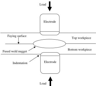
Figure 2.1: Illustration of resistance spot welding process
The dominance of RSW in the automotive structural assemblies can be seen on a typical body-in-white which contains a very large number of spot welds. Therefore, the reliability of the spot welds hence determines the structural performance of a body-in-white. Nevertheless, liked bolted joints, thorough characterization of spot weld behaviour is important and always of concern owing to the fact that the inherent behaviour of spot welds such as geometrical irregularities, residual stresses, material inhomogeneity and defects are difficult to replicate in finite element modelling (Mottershead et al., 2006). However, because of a large number of spot welds in automobile structures, it is often impractical to model each or every spot weld joint in details. Therefore reliable procedures and methods that could be used to represent spot weld joints in automobile structures in the simplest way have been of interest for the last few decades. In other words the simplified models should be able to deliver reliable results of any analysis interest.
Faying surface
Fused weld nugget Bottom workpiece
Top workpiece
Indentation
Load
Electrode
In years before the 1980s, theoretical modelling of spot weld was not mature. For example, publications of theoretical modelling of the resistance spot welding in the decade of 1967 to 1977 were sparse (Nied, 1984). Consequently, most of research work on spot welded structures was carried out experimentally. By and large, the work was mainly focused either on the fatigue and the static strength of spot welds (Jourmat and Roberts, 1955 ; Orts, 1981 and Rossetto, 1987). However, since early 1990s numerous attempts have been progressively made to improve the previous approach by adopting numerical techniques for modelling spot welds. There is a large number of people who worked on this subject and some of them are Lim et al. (1990); Vopel and Hillmann (1996); Blot (1996); Heiserer et al. (1999); Palmonella et al. (2003); De Alba et al. (2009); Abu Husain et al. (2010b) and etc.
Modelling work associated with spot welds can be categorised into two major groups. The first category belongs to models for limit capacity analysis (Deng et al., 2000) and the second one belongs to models for dynamic analysis (Fang et al., 2000) which the application of ACM2 and CWELD model was reported to be the predominant approach for dynamic analyses in automotive industry (Palmonella et al., 2004). Due to the fact of the complexity of spot weld behaviour, the former requires a very detailed models which are important to capture stress concentrations and hence particular emphasis is placed on modelling sudden geometry changes.
Study of dynamic characteristics of structures is usually treated as a global issue rather than a local issue owing to the fact that eigenproblem is typically a function of the structural mass and stiffness and of the boundary conditions as well. However, when it comes to investigating eigenproblem of welded structures, emphasis should not only be on modelling work of the structure but also be on spot weld modelling. This is because the properties and characteristics of spot welds play a significant role in the dynamic behaviour of welded structures. In other words, dynamic characteristics of numerical models of welded structures highly depend on the quality and reliability of spot weld model. The well accepted alternative method for modelling spot welds in the past few decades was to use coincident nodes approach through which the nodes were coincident at boundary between the welded components (Lardeur et al., 2000). However, since early 1990s single beam models have been commonly used in modelling spot welds in industries. Rigid bar and elastic rod element are categorised into these single beam models. They are used to connect between two nodes of adjoining meshed sheets and their descriptions of connection and usage are available in (MSC.2., 2010).
Further demonstration of the application of single beam elements in representing resistance spot welds was performed by Vopel and Hillmann (1996) and Blot (1996). It was then followed by Lardeur et al. (2000) who also used single beam elements in studying the best predictive spot weld model for vibrational behaviour of automotive structure. The Investigation on spot weld modelling using single beam elements was continued by Fang et al. (2000). They demonstrated the numerical problems with spot weld connections modelled with single beam elements.
Meanwhile, Donders et al. (2005) particularly in one of the sections of their paper, discussed the accuracy of results calculated from spot weld connections modelled as single beam elements. However, none of the aforementioned attempts to use single beam elements to model spot welds had produced satisfactory results of dynamic behaviour of welded structures. Common conclusions made in their studies were that spot weld connections modelled as single beam elements would only produce unsatisfactory results in comparison with those experimentally observed and the drawbacks of single beam elements representing the physical spot welds lie in several factors. The factors were summarised by Heiserer et al. (1999) as follows:
Shell elements with rotational stiffness are not strong enough to resist the
rotations introduced by elements such as beams or springs. A singularity is introduced in the shell area. The model does not run without PARAM, K6ROT and PARAM, SNORM.
Beam elements, or even worse, bar elements are used whose diameter is
CQUAD4 and CTRIA3 shell elements, only have five degrees of freedom, the sixth degree of freedom which is the rotational degree of freedom (R3) about a
vector normal to the shell element at each GRID point (sometimes called the
drilling degree of freedom), has zero stiffness. Therefore, PARAM, K6ROT
defines a multiplier to a fictitious stiffness to be added to the out of plane rotation
stiffness of CQUAD4 and CTRIA3 elements. For linear solutions (all solution
sequences except SOLs 106 and 129), the default value for K6ROT is equal to zero
and it can be defined in NASTRAN as PARAM, K6ROT, 0. In most instances, the
default value should be used.
Figure 2.2: Unique grid point normal for adjacent shell elements
PARAM, SNORM defines a unique direction for the rotational degrees of freedom
of all adjacent elements (CQUAD4 and CTRIA3). A shell normal vector is created
by averaging the normal vectors of the attached elements. In this example, shell
normals are used if the actual angle, , between the local element normal and the
unique grid point normal is less than 20 degrees (see Figure 2.2).
In linear solution sequences, the values of PARAM, K6ROT, 0 and PARAM,
SNORM, 20 are recommended (MSC.5., 2004).
Shell 1 Shell 2
Grid point normal
Shell 2 normal Shell 1 normal
The pitfalls had attracted attention of a number of people to come out better ways of representing numerically physical spot welds. Heiserer et al. (1999) proposed another type of spot weld model namely Area Contact Model 2 (ACM2). The surface contact model was constructed based on HEXA solid element and RBE3 interpolation elements that were used to link the HEXA model with the nodes of shell elements. The advantages of this spot weld model is that it can be used for both limit capacity analysis and dynamic analysis. Another beneficial gain from the model is that it allows the model to be used for congruent and non-congruent component meshes.
The advantages of the model in several aspects have caused an attention to a large number of the people either from academia or industry to use it in their research and development work. For example, Lardeur et al. (2000) successfully used ACM2 to represent physical spot welds and predicted the dynamic behaviour of both academic welded structure and automotive welded structure in comparison with the measured results. Another good example of using ACM2 in predicting the dynamic behaviour of welded structure was performed by Palmonella et al. (2003). Apart from using ACM2 to represent the spot welds, they also demonstrated model updating work on the spot weld model and the effect of considering patch as updating parameter on the accuracy of the updated model. Meanwhile a compressive overview of ACM2 in term of the application of the model in NVH and durability analysis in automotive industry was give by Donders et al. (2005) and Donders et al. (2006). The effect of refinement of the welded structure meshes on the accuracy of the analysis results calculated from ACM2 was elaborated and presented by Torsten and Rolf (2007).
welding process, therefore the Young's modulus of parent material is used for that of CWELD element. Apart from being able to be used for connecting both congruent and non-congruent meshes, CWELD element also can be defined in three types of connections with five different formats:
A Point to Point connection, where an upper and lower shell grid are
connected. This type of connection can be defined with ALIGN format
A Point to Patch connection; where a grid point of a shell is connected to a
surface patch. This connection can be defined with format in ELEMID and GRID
A Patch to Patch connection, where a spot weld grid GS is connected to an
upper and lower surface patch. It can be defined with PARTPAT, ELPAT, ELEMID and GRID. However, ELPAT or PARTPART is the most flexible format in comparison with the other two.
of patch which is normally 3x3 elements per patch. The same spot weld modelling technique was used by Palmonella et al. (2003) ; Palmonella et al. (2004) and Palmonella et al. (2005) for investigating and improving dynamic behaviour of a welded beam that is comprised of a hat and a plate welded together by twenty spot welds. CWELD elements with the type of connection of patch to patch were used to model the spot welds. The discrepancies between the initial model of the welded beam and the tested structure were assumed to be due to the invalid assumptions of the parameters of spot welds. In the investigation, they concluded that CWELD modelling technique showed a high capability of and the simplest method for representing spot welds. On top of that, the optimum size and also the Young's modulus of patch of CWELD element had play a significant role in improving the accuracy of the predicted results through the application of model updating.
The requirement of detailed finite element models highly depends on the type of analysis concerned. The more detailed the finite element models are the more elements on the models would there be and the much longer computational time is required. Therefore, the detail of finite element models is a trade-off between accuracy and expenditure of computational time. Owing to the fact, it is always to be a high desire for CAE engineers in automotive industry to have the same finite element model mesh for durability, crashworthiness and NVH analysis. However, the sort of the analyses, in practice, requires different finite element model meshes, especially crashworthiness analysis that needs detailed finite element models.