Bivariate random-effects meta-analysis and the estimation of between-study correlation

(1)

BioMed Central

Page 1 of 15 (page number not for citation purposes)

BMC Medical Research

Methodology

Open Access

Research article

Bivariate random-effects meta-analysis and the estimation of

between-study correlation

Richard D Riley*

1

_{, Keith R Abrams}

2

_{, Alexander J Sutton}

2

_{, Paul C Lambert}

2

and John R Thompson

2

Address: 1_{Centre for Medical Statistics and Health Evaluation, School of Health Sciences, University of Liverpool, Shelley's Cottage, Brownlow} Street, Liverpool, L69 3GS, UK and 2_{Centre for Biostatistics and Genetic Epidemiology, Department of Health Sciences, University of Leicester, 2nd} Floor, Adrian Building, University Road, Leicester, LE1 7RH, UK

Email: Richard D Riley* - [email protected]; Keith R Abrams - [email protected]; Alexander J Sutton - [email protected]; Paul C Lambert - [email protected]; John R Thompson - [email protected]

* Corresponding author

Abstract

Background: When multiple endpoints are of interest in evidence synthesis, a multivariate meta-analysis can jointly synthesise those endpoints and utilise their correlation. A multivariate random-effects meta-analysis must incorporate and estimate the between-study correlation (ρ_B).

Methods: In this paper we assess maximum likelihood estimation of a general normal model and a generalised model for bivariate random-effects meta-analysis (BRMA). We consider two applied examples, one involving a diagnostic marker and the other a surrogate outcome. These motivate a simulation study where estimation properties from BRMA are compared with those from two separate univariate random-effects meta-analyses (URMAs), the traditional approach.

Results: The normal BRMA model estimates ρB as -1 in both applied examples. Analytically we show this

is due to the maximum likelihood estimator sensibly truncating the between-study covariance matrix on the boundary of its parameter space. Our simulations reveal this commonly occurs when the number of studies is small or the within-study variation is relatively large; it also causes upwardly biased

between-study variance estimates, which are inflated to compensate for the restriction on B. Importantly, this

does not induce any systematic bias in the pooled estimates and produces conservative standard errors and square errors. Furthermore, the normal BRMA is preferable to two normal URMAs; the mean-square error and standard error of pooled estimates is generally smaller in the BRMA, especially given data missing at random. For meta-analysis of proportions we then show that a generalised BRMA model is better still. This correctly uses a binomial rather than normal distribution, and produces better estimates than the normal BRMA and also two generalised URMAs; however the model may sometimes not converge due to difficulties estimating ρ_B.

Conclusion: A BRMA model offers numerous advantages over separate univariate synthesises; this paper highlights some of these benefits in both a normal and generalised modelling framework, and examines the estimation of between-study correlation to aid practitioners.

Published: 12 January 2007

BMC Medical Research Methodology 2007, 7:3 doi:10.1186/1471-2288-7-3

Received: 4 September 2006 Accepted: 12 January 2007

This is an Open Access article distributed under the terms of the Creative Commons Attribution License (http://creativecommons.org/licenses/by/2.0), which permits unrestricted use, distribution, and reproduction in any medium, provided the original work is properly cited.

ˆ

(2)

Background

Traditionally, meta-analysis models combine summary measures of a single quantitative endpoint, taken from different studies, to produce a single pooled result. How-ever, multiple pooled results are required whenever there are multiple outcomes [1] or multiple treatment groups [2]. A multivariate meta-analysis model uses the correla-tion between the endpoints and obtains the multiple pooled results collectively [3,4]. For example, Reitsma et al. [5] have suggested a bivariate random-effects meta-analysis (BRMA) to jointly synthesise logit-sensitivity and logit-specificity values from diagnostic studies. Multivari-ate meta-analysis has been quite widely used, including application to genetic associations [6], surrogate end-points [7,8], psychological findings [9] and prognostic markers [10].

Often the advantage of a multivariate random-effects meta-analysis lies in its ability to use the between-study correlation of the multiple endpoints of interest. For example, in diagnostic studies the sensitivity and specifi-city are usually negatively correlated across studies due to the use of different thresholds [5]. Van Houwelingen et al. [4] use the between-study correlation to describe the shape of the bivariate relationship between the true log-odds in a treatment group and the true log-log-odds in a con-trol group (baseline risk). Riley et al. [10] algebraically assess BRMA and show that the correlation allows a 'bor-rowing of strength' across endpoints. This leads to pooled estimates that have a smaller standard error than those from corresponding univariate random-effects meta-anal-yses (URMAs), especially when some endpoints are miss-ing at random across studies.

Some recent articles have indicated the between-study cor-relation may often be estimated at the end of its parameter space, as +1 or -1. Thompson et al. [6] apply a normal BRMA model to genetic studies of coronary heart disease and report that the between-study correlation was 'poorly estimated' with the likelihood peaking at +1, and an esti-mate of +1 has also been reported in other applications [4,11]. To aid practitioners, in this paper we analytically consider why this occurs, and then explore the impact, if any, this has on the pooled estimates and between-study variance estimates. This investigation also allows us to examine the general benefits of BRMA over URMA, to build on a number of other recent articles [5,10], and encourage a greater use and appreciation of BRMA in prac-tice.

The outline of the paper is as follows. We begin by intro-ducing the general normal model for BRMA and discuss analytically why the between-study correlation can be estimated at the edge of its parameter space. We then apply the model to two real examples from the literature,

one involving a diagnostic marker and one involving a surrogate outcome, and these both give a between-study correlation estimate of -1. This then motivates a realistic simulation study to examine how the estimate of between-study correlation affects the statistical properties of the pooled and between-study variance estimates. It also allows us to compare the performance of the normal BRMA model to two separate URMAs, the more common approach in practice [10]. We then extend our work to consider meta-analysis of proportions, and highlight why a generalised model for BRMA is preferred to the general normal BRMA model [12], and also two separate general-ised URMA models. We conclude by summarising the broad benefits of BRMA for practitioners, and discuss future research priorities.

Methods

In this section we introduce a hierarchical normal frame-work for BRMA and URMA. We describe how the BRMA normal model is estimated, and analytically consider the estimation of between-study correlation. We then describe the rationale and methodology for our simula-tion study of BRMA versus URMA. To ensure a real world context, this section also includes two motivating exam-ples from the medical literature where a BRMA is poten-tially important.

Motivating example 1 – the telomerase data

Glas et al. [13] systematically review the sensitivity and specificity of tumour markers used for diagnosing primary bladder cancer. One of these markers was telomerase, a ribonucleoprotein enzyme, evaluated in 10 studies as shown in Table 1. Rather than applying a URMA inde-pendently for sensitivity and specificity, the authors jointly synthesise the logit-transformed sensitivity and the logit-transformed specificity in a normal BRMA model as described below and recently proposed elsewhere [5].

A general normal model for bivariate random-effects meta-analysis (BRMA)

(3)

BMC

Med

ical Rese

arch Me

th

odol

ogy

200

7,

7

:3

http://www.bi

omedcen

tr

al

.co

m

/14

71-22

88/7/3

Pa

ge 3 of

1

5

(page nu

mber not

for

cit

a

tion pur

[image:3.612.52.753.85.503.2]

poses)

Table 1: The telomerase data taken from the bladder cancer review of Glas et al. [13]

Study Number of patients with bladder cancer

Number of patients with bladder cancer

and a positive test result

Sensitivity Logit-sensitivity Y_i₁ Standard error of logit-sensitivity S_i₁

Number of patients without bladder cancer

Number of patients without

bladder cancer and a negative

test result

Specificity Logit-specificity Y_i₂ Standard error of logit-specificity S_i₂

Within-study correlation ρ_Wi

1 33 25 0.758 1.139 0.406 26 25 0.962 3.219 1.020 0

2 21 17 0.810 1.447 0.556 14 11 0.786 1.299 0.651 0

3 104 88 0.846 1.705 0.272 47 31 0.660 0.661 0.308 0

4 26 16 0.615 0.470 0.403 83 80 0.964 3.283 0.588 0

5 57 40 0.702 0.856 0.290 138 137 0.993 4.920 1.004 0

6 47 38 0.809 1.440 0.371 30 24 0.800 1.386 0.456 0

7* 43 23.5 0.547 0.187 0.306 13 12.5 0.962 3.219 1.442 0

8 33 27 0.818 1.504 0.451 20 18 0.900 2.197 0.745 0

9 17 14 0.824 1.540 0.636 32 29 0.906 2.269 0.606 0

10 44 37 0.841 1.665 0.412 29 7 0.241 -1.145 0.434 0

(4)

assumed normally distributed then the BRMA can be specified as:

This model is the general normal model for BRMA [4], where δ_iand Ω are the within-study and the between-study covariance matrices respectively. Usually of key interest from the analysis are the pooled estimates of β₁ and β₂, although sometimes an estimated function of these may be desired; for instance in the telomerase exam-ple an estimate of the log of the diagnostic odds ratio is given by 1 + 2. The BRMA differs from two independ-ent URMAs by the inclusion of the within-study correla-tions (i.e. the ρWi s) and the between-study correlation (ρ_B). Equation (2) is equivalent to two independent URMAs when ρWi = ρB = 0 for all i, i.e. there is zero corre-lation:

In equation (1) it is common to assume the s and ρ_Wi

s are known [1,4]. Including the uncertainty of the s is unnecessary for URMA [14], but whether the uncertainty of the s and ρ_Wis should be incorporated in BRMA is yet to be examined. This issue is outside the scope of this paper but we note that a Bayesian framework is particu-larly flexible for incorporating such uncertainty [15].

Within- and between-study correlation

The within-study correlation, ρ_Wi, indicates whether Y_i₁and

Y_i₂are correlated within a study, and these ρ_Wis are usu-ally assumed known. For the telomerase data the ρ_Wis might be assumed to be zero because sensitivity and spe-cificity values are calculated independently in a study using different sets of patients. In other BRMA applica-tions the ρ_Wis can be non-zero, for example where the two endpoints are overall and disease-free survival [10]. In practice it may be difficult to obtain the value of non-zero

ρ_Wis, although it can be done as evident in Berkey et al. [1] and the 'motivating example 2' below [7]. Suggestions for limiting the problem of unavailable ρ_Wis have been proposed [15-17], and this issue is considered further in the discussion.

The between-study correlation, ρB, is not generally known

and has to be estimated when fitting the BRMA. It indi-cates how the underlying true values, i.e. the θ_i₁s and the θ_i₂s, are related across studies. It may be caused by differ-ences across studies in patient-level characteristics, such as age and stage of disease, or changes in study-level charac-teristics, such as the threshold level in diagnostic studies

Motivating example 2 – the CD4 data

Daniels and Hughes [7] assess whether the change in CD4 cell count is a surrogate for time to either development of AIDS or death in drug trials of patients with HIV. They consider between-treatment-arm log-hazard ratios of time to onset of AIDS or death (Yi1), and between-treatment-arm differences in mean changes in CD4 count (Y_i₂) from pre-treatment baseline to about six months. Fifteen rele-vant trials were identified. Some of the trials involved three or four treatment arms, but to enable application to BRMA here we only consider outcome differences between the control arm and the first treatment arm in the reported dataset [7]. All fifteen trials provided complete data, including the within-study correlations which were quite small, varying between -0.22 and 0.17 with a mean of -0.08.

Estimation

In our analyses of equation (1) in this paper the between-study parameters (i.e. , and ρ_B) and the two pooled values (β₁and β₂) are estimated iteratively using restricted maximum likelihood (REML) in SAS Proc Mixed, as described elsewhere [4]. Unless otherwise stated, we also use Cholesky decomposition [18] of Ωto ensure that this matrix is estimated to be positive semi-definite and there-fore that the between-study correlation estimate, _B, is in the range [-1,1]. Cholesky decomposition of Ωalso helps ensure convergence when _Bis very close to 1 or -1.

Analytic consideration of the between-study covariance parameters

Estimation and inference in classical linear mixed models are based on the marginal model, which for equation (1) is the bivariate normal model with variance-covariance δ_i + Ω. Assume for the sake of simplicity that the within-study covariance matrix δ_i= δfor all studies. Then the cov-ariance matrix of the observed Yi1 s and Yi2 s is given by V = δ+ Ω, where δis known. Now, this puts (severe) restric-Y

Y N

s s s

s s i

i

i i i

i i i wi

i i 1 2 1 2 1 2 1 2 1 ⎛ ⎝ ⎜ ⎞ ⎠ ⎟ ⎛ ⎝ ⎜ ⎞ ⎠ ⎟ ⎛ ⎝ ⎜⎜ ⎞_⎠⎟⎟ =

~ θ ,

θ

ρ δδ δδ

2

2 22

1

2

1

2

12 1

ρ θ θ β β τ τ wi i i i s N ⎛ ⎝ ⎜ ⎜ ⎞ ⎠ ⎟ ⎟ ⎛ ⎝ ⎜ ⎞ ⎠ ⎟ ⎛ ⎝ ⎜ ⎞ ⎠ ⎟ ⎛ ⎝ ⎜⎜ ⎞_⎠⎟⎟ =

~ ,ΩΩ ΩΩ ττ ρ

τ τ ρ τ

2

1 2 22

1 B B ⎛ ⎝ ⎜ ⎜ ⎞ ⎠ ⎟ ⎟

( )

ˆ

β _βˆ

Y Y N s s i i i

i i i i i 1 2 1 2 1 2 2 2 0 0 ⎛ ⎝ ⎜ ⎞ ⎠ ⎟ ⎛ ⎝ ⎜ ⎞ ⎠ ⎟ ⎛ ⎝ ⎜⎜ ⎞_⎠⎟⎟ =⎛ ⎝ ⎜ ⎜ ⎞ ⎠ ⎟ ⎟

~ θ ,

θ δδ δδ

θθ θ β β τ τ i i N 1 2 1 2 12 22 0 0 2 ⎛ ⎝ ⎜ ⎞ ⎠ ⎟ ⎛ ⎝ ⎜ ⎞ ⎠ ⎟ ⎛ ⎝ ⎜⎜ ⎞_⎠⎟⎟ =⎛ ⎝ ⎜ ⎜ ⎞ ⎠ ⎟ ⎟

( )

~ ,ΩΩ ΩΩ

s_ij2

τ12 τ22

ˆ

ρ

ˆ

(5)

BMC Medical Research Methodology 2007, 7:3 http://www.biomedcentral.com/1471-2288/7/3

tions on V, namely that V - δis a covariance matrix, that is non-negative definite. If the estimated V does not satisfy this restriction, the maximum likelihood estimate of Ω will be truncated on the boundary of its parameter space. This means that if Ωis diagonal (as for URMA) the maxi-mum likelihood estimate on the boundary will have one or both of the between-study variances equal to zero; else if Ω is non-diagonal (as for BRMA) then either one or both of the between-study variances equals zero or else the between-study correlation equals -1 or +1. In meta-analysis a between-study variance estimate of zero is wellunderstood, but a betweenstudy correlation estimate of -1 or +-1 is likely to be less familiar to practitioners. Thomp-son et al. [6] refer to this issue as 'poor estimation' but it perhaps should rather be considered a natural conse-quence of the sensible restrictions imposed on V, and one that prevents a variance estimate < 0 or a correlation esti-mate > +1 or < -1, as might otherwise be obtained.

Rationale for the research in this paper

In this paper, to aid practitioners we will further assess the normal BRMA model and the role of between-study corre-lation. In particular, we aim to identify the situations when _Bis likely to be +1 or -1 and examine the impact this has on the pooled and between-study variance esti-mates. We will also evaluate the benefits of BRMA over two separate URMAs, the more common approach in

practice, and explore extensions to a generalised BRMA model for meta-analysis of proportions. To achieve these goals we firstly apply the normal BRMA of equation (1) to the two motivating examples. We then perform a simula-tion study of the normal BRMA model, as described below. The generalised BRMA model is then introduced and assessed in relation to the normal BRMA model and two separate generalised URMAs (see Results).

A simulation study to assess BRMA and the between-study correlation

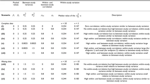
We carried out a simulation study of the general normal model for BRMA in 11 scenarios, labelled (i) to (xi) (Table 2). Each of scenarios (i) to (xi) relates to a different but realistic specification of equation (1). Scenarios (i) to (vi) consider complete data, as in the telomerase example, whereas scenarios (vii) to (vi) consider when some data are missing at random across studies, as assumed in the BRMA of Thompson et al. [6]. The scenarios also vary in the relative sizes of the within- and between-study corre-lations, and also the within- and between-study variation. For example, scenarios (i) to (iv) involve within-study var-iances similar in size to the between-study varvar-iances, as observed in prognostic studies [10], and in scenario (vi) there is one relatively low and one relatively high between-study variance, as for the CD4 dataset. The sizes of the meta-analysis were either n = 5 or n = 50 studies for complete data, and either n = 10 or n = 50 for missing ˆ

[image:5.612.54.551.447.726.2]

ρ

Table 2: Scenarios used in the simulations based on equation (1)

Pooled values

Between-study variances

Within- and between-study

correlation

Within-study variation

Scenario β1 β2 ρWi ρB Median value of the s: Description

Complete data n = 50 n = 5

(i) 0 2 0.25 0.25 0 0 0.254 0.147 Zero correlation; within-study variation similar to between-study variation

(ii) 0 2 0.25 0.25 0 0.8 0.254 0.147 No within-study correlation but high between-study correlation; within-study variation similar to between-study variation

(iii) 0 2 0.25 0.25 0.8 0 0.254 0.147 High within-study correlation but no between-study correlation; within-study

variation similar to between-study variation

(iv) 0 2 0.25 0.25 0.8 0.8 0.254 0.147 High within- and between-study correlation; within-study variation similar to between-study variation

(v) 0 2 0.0025 0.0025 0.8 0.8 0.254 0.147 High within- and between-study correlation; within-study variation large relative to between-study variation

(vi) 0 2 0.0025 1.5 0.8 0.8 0.254 0.147 High within- and between-study correlation; within-study variation large (for endpoint 1) and small (for endpoint 2) relative to between-study variation

(vii) 0 2 1.5 1.5 0.8 0.8 0.254 0.147 High within- and between-study correlation; within-study variation small

relative to between-study variation

Missing data n = 50 n = 10

(viii) 0 2 1.5 1.5 0 0.8 0.244 0.183 No within-study correlation but high between-study correlation; within-study

variance small relative to between-study variance

(ix) 0 2 0.25 0.25 0 0.8 0.244 0.183 No within-study correlation but high between-study correlation; within-study variance similar to between-study variance

(x) 0 2 1.5 1.5 0.8 0.8 0.244 0.183 High within- and between-study correlation; within-study variance small relative to between-study variance

(xi) 0 2 0.25 0.25 0.8 0.8 0.244 0.183 High within- and between-study correlation; within-study variance similar to between-study variance

(6)

data. Our method of simulation was deliberately chosen to be similar to that previously used by Berkey et al. [1] and Sohn [19]. As an example, we now describe the simu-lation procedure for scenario (i) with n = 50.

Description of the simulation procedure for scenario (i) with n = 50

Generation of a dataset of 1000 meta-analyses

We chose β₁= 0 in order to reflect little clinical benefit (e.g. a sensitivity of 50%) and in contrast β₂= 2 (e.g. a spe-cificity of 88%). The within study variances required, i.e. the 50 s and 50 s, were each found by sampling from a N(0.25,0.50) distribution and squaring the value obtained. This produced a median of 0.25 and an interquartile range of 0.7, values similar to those for the telomerase data (median = 0.21) and for the BRMA of

Thompson et al. [6] (median = 0.28, interquartile

range = 0.76). The between-study variances, and , were chosen to be 0.25 in scenario (i), which meant that they were similar in size to the median within-study vari-ances. The within and between-study correlations were both set to zero for this scenario. All these choices were substituted into equation (1) and 1000 meta-analyses each of 50 studies were generated. Calculations were per-formed in S-Plus using the 'rmvnorm' function for gener-ating bivariate normal values (code available upon request).

Estimation using the dataset of 1000 meta-analyses

Each of the 1000 meta-analyses in scenario (i) were ana-lysed separately by:

• fitting two separate URMAs as in equation (2) (where ρ_B = 0) using REML to estimate β₁, β₂, and

• fitting a BRMA as in equation (1) using REML to esti-mate β1, β2, , , and ρB

The 1000 BRMA estimates and the corresponding 1000 URMA estimates from scenario (i) were then compared by calculating:

• average parameter estimates across all the simulations (to check for bias)

• coverage of the 95% confidence intervals for β₁and β₂

• average standard error and mean-square error (MSE) of β₁and β₂

• the number of occasions _Bwas equal to +1 or -1 in the BRMA

To assess coverage, the 95% confidence intervals for β_j were calculated using:

with n_jthe number of studies providing endpoint j. This t -distribution is commonly used in the meta-analysis liter-ature, although it is only an approximation [20].

Description of the simulation procedure for scenarios (ii) to (xi)

Simulations in the other scenarios followed in the same manner as described above but with the data generated from the parameter values specific to each scenario as given in Table 2. For those missing data simulations of scenarios (viii) to (xi) we simulated data as described for complete data, except that for each generated meta-analy-sis we removed the data for the second endpoint in a ran-domly selected 50% of studies. So, for example, with n = 50 in scenario (viii) each of the 1000 simulated meta-analyses contained 25 studies with complete data and 25 studies with data for the first endpoint only.

Results

Application to the telomerase and CD4 data

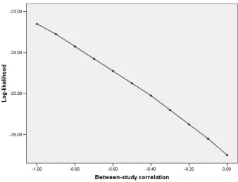
The normal model for BRMA (equation (1)) and then two separate URMAs (equation (2)) were applied to the tel-omerase data. Both approaches gave a pooled sensitivity of about 76% and a pooled specificity of about 88% (Table 3). The BRMA gave a between-study correlation estimate of -1 but the profile likelihood reveals that there is little information regarding ρ_Bwith the log-likelihood gradually increasing as _Bapproaches -1 (Figure 1), the end of its parameter space. Interestingly, the between-study variances were estimated to be somewhat larger in the BRMA than the URMA, and the standard errors of the pooled estimates were also slightly larger in the BRMA; just the opposite of what one might expect from a bivari-ate analysis utilising large correlation [10]. A similar find-ing was observed upon application of BRMA and URMA to the CD4 data. The BRMA again gave a between-study correlation estimate of -1 and both between-study vari-ances were estimated somewhat larger in the BRMA than the URMA, as were the standard errors of the pooled esti-mates.

s_i2₁ s_i2₂

sij2

s_ij2

τ12 τ22

ˆ

ρ

ˆ _{( .} ₎ _{( ˆ ) ,}

βj±

(

tn_j−10 05 ∗ var βj

)

ˆ

(7)

The question is thus posed: is the estimation of ρ_Bat the boundary of its parameter space adversely influencing the other BRMA parameter estimates and, if so, how (e.g. does it introduce bias)? Also, in terms of the individual pooled estimates, the telomerase and CD4 examples indicate lit-tle benefit of BRMA over two separate URMAs, despite the utilisation of correlation; but is this generally true and in what situations should a BRMA be preferred? To under-stand the answers to these important questions, it is help-ful to now consider the results from our simulation study.

We note at this point that, for both telomerase and CD4, we also tried estimation of BRMA using an unstructured form of Ω, rather than using Cholesky decomposition of

Ω as previously. Interestingly, this approach produced non-sensical between-study correlation estimates of -1.12 and -1.074 for the telomerase and CD4 datasets respec-tively. This emphasises the importance of a boundary con-straint on ρ_Bas imposed by the Cholesky decomposition.

Profile log-likelihood for the between-study correlation from the general normal BRMA of the telomerase data Figure 1

[image:7.612.134.473.422.681.2]

Profile log-likelihood for the between-study correlation from the general normal BRMA of the telomerase data.

1

Table 3: URMA and BRMA results for the telomerase and CD4 datasets

Dataset Model _{Pooled value}

endpoint 1 1

(s.e.)

Between-study variance endpoint

2

Pooled value

endpoint 2 2

(s.e.)

Between-study variance endpoint

2

Between-study

correlation B

Telomerase Normal URMA 1.155 (0.186) 0.186 1.964 (0.541) 2.386 NA

Normal BRMA 1.166 (0.186) 0.202 2.058 (0.554) 2.584 -1.0

Generalised URMA

1.182 (0.176) 0.155 2.215 (0.578) 2.680 NA

CD4 Normal URMA -0.049 (0.0695) 0.025 17.300 (5.561) 379.73 NA

Normal BRMA -0.109 (0.0748) 0.048 18.314 (5.740) 412.96 -1.0

s.e. = standard error; NA = not applicable; 95% confidence interval calculated using t-distribution with 9 degrees of freedom. Restricted maximum likelihood estimation was used for the normal models, whereas maximum likelihood estimation was used for the generalised model.

ˆ

β

ˆ

τ12

ˆ

β

ˆ

τ22

ˆ

(8)

Simulation results

Table 4 includes the simulation results for scenarios (i), (ii), (viii) and (ix). The results for all other scenarios are provided in Appendix 1 (see Additional file 1). We now discuss the key findings.

Between-study correlation

One can see from Table 4 that the normal model for BRMA often estimates the between-study correlation, ρ_B, as either +1 or -1, especially when the number of studies in the meta-analysis is small. For example, with n = 5 in scenario (ii), where the true ρ_Bwas 0.8, 605 of the 1000 simulations (60.5%) gave _Bequal to +1 and 103 simu-lations (10.3%) gave _Bequal to -1. This led to a mean value of _Bequal to 0.639, a downward bias of about 20%. However, this downward bias is not in itself a con-cern because it is simply caused by the maximum likeli-hood estimator sensibly truncating _Bat +1 and -1, which improves the mean-square error of _B. Further-more, _Bis clearly asymptotically unbiased, with the occurrence of _Bequal to -1 or +1 and thus the bias in mean _Bbecoming increasingly less as the number of studies in the meta-analysis increases (Table 4). Interest-ingly though, the number of studies required to reduce the occurrence of _Bequal to -1 or +1 was far greater when the within-study variation was large relative to the between-study variation. For example, even with a large n

= 50 studies in scenario (v), where the within-study

varia-tion was relatively large, 58% of the simulavaria-tions gave a between-study correlation of -1 or +1.

These findings indicate why _Bequals -1 in the BRMAs of the telomerase and CD4 datasets. For the telomerase data there are 10 studies; the simulations show that this mag-nitude of studies will often provide little information about ρ_B, causing _Bto often be constrained at -1 or +1 so that the restrictions imposed on V are met. For the CD4 data, even though there are five more studies than telom-erase, the mean within-study variance for endpoint j = 1 is 0.15 and this is large relative to the between-study varia-tion ( = 0.048). In such situations where the within-study variation dominates, the simulations again show that _Bwill often require truncation at the end of its parameter space to ensure V is non-negative definite.

Between-study variance estimates

Our simulation results show that the between-study vari-ance estimates were less frequently truncated at zero in the BRMA than the URMA (Table 4). For example, in scenario (ii) with n = 5 was zero for 104 of the URMA simula-tions and none of the BRMA simulasimula-tions. Furthermore, in those scenarios where the between-study correlation was often +1 or -1 (e.g. scenario (ii) with n = 5), the normal BRMA model produces a noticeable upward bias in the between-study variance estimates. For example, in sce-nario (ii) with n = 5 there was an upward bias of 0.024 in and , about 10% above their true value. To under-stand analytically why this occurs, we need to consider that the between-study covariance (τ12) is formulated by τ₁₂= ρ_Bτ₁τ₂. Now, if _Bis constrained at -1 or +1, then to obtain the necessary solution for ₁₂the maximum like-lihood estimator can only increase the j s, which do not have an upper bound constraint. Thus the between-study variance estimates are inflated to compensate for the con-straint on _B. This explains why the BRMAs of the telom-erase and CD4 data, where _Bwas truncated at -1, give _j s that are noticeably larger than those from two separate URMAs. Practitioners need to be aware of this issue; how-ever, we do not consider it a major concern as the maxi-mum likelihood estimator for is still asymptotically unbiased (the bias decreases as the number of studies increases) and the inflation is simply caused by the sensi-ble and necessary constraint on _B. Furthermore, the inflation is essentially conservative, leading to a larger standard error and mean-square error of pooled estimates as now discussed.

Pooled estimates

For all complete and missing data scenarios, the pooled estimates were approximately unbiased for both BRMA and URMA. Even in those scenarios where _Bwas often + 1 or -1 it is encouraging that, despite the upward bias in between-study variances, there was no systematic bias in the pooled estimates from the BRMA (Table 4 and Appen-dix 1 – see Additional file 1). The main affect on the pooled estimates was an inflated standard error and mean-square error. This is a conservative property, but meant that in some complete data scenarios the BRMA performed slightly worse than URMA, despite the utilisa-tion of correlautilisa-tion in the BRMA that might be expected to improve efficiency [10]. For example, in the n = 5 results ˆ

ρ

ˆ

ρ

ˆ

ρ

ˆ

ρ

ˆ

ρ

ˆ

ρ

ˆ

ρ

ˆ

ρ

ˆ

ρ

ˆ

ρ

ˆ

ρ

ˆ

τ12

ˆ

ρ

ˆ

τ22

ˆ

τ12 τˆ22

ˆ

ρ

ˆ

τ

ˆ

τ

ˆ

ρ

ˆ

ρ _τˆ

τj2

ˆ

ρ

ˆ

(9)

BMC

Med

ical Rese

arch Me

th

odol

ogy

200

7,

7

:3

http://www.bi

omedcen

tr

al

.co

m

/14

71-22

88/7/3

Pa

ge 9 of

1

5

(page nu

mber not

for

cit

a

tion pur

[image:9.612.65.746.79.532.2]

poses)

Table 4: Simulation results of the normal BRMA and URMA models for scenarios (i), (ii), (viii), and (ix)

Meta-analysis model

n No. of the 1000 simulations

that converged

Bias of mean

1

Mean s.e. of

1

MSE of

1

Coverage of the

95% CIs for 1

2

MSE of

2

Coverage of the 95%

CIs for 2

Bias of mean

(no. of = 0)

Bias of mean

(no. of = 0) Bias of

mean

B

% of B = -1 % of B = 1

Scenario (i): Complete data – zero correlation; within-study variance similar to between-study variance

URMA 50 1000 -0.005 0.102 0.010 94.8% 0.001 0.107 0.0108 95.4% -0.003 (0) 0.005 (1) - -

-BRMA 50 1000 -0.005 0.101 0.010 94.7% 0.001 0.106 0.0108 95.5% -0.003 (0) 0.005 (0) -0.001 0.2% 0.4%

URMA 5 1000 -0.002 0.267 0.081 96.0% -0.006 0.267 0.0887 94.0% -0.006 (89) 0.015 (81) - -

-BRMA 5 998 -0.002 0.274 0.081 96.7% -0.006 0.269 0.0894 95.3% 0.008 (10) 0.024 (0) -0.027 29.6% 29.0%

Scenario (ii): Complete data – no within-study correlation, high between-study correlation; within-study variance similar to between-study variance

URMA 50 1000 -0.004 0.102 0.010 95.6% 0.001 0.106 0.0114 94.4% 0 (0) -0.004 (1) - -

-BRMA 50 1000 -0.004 0.100 0.010 95.3% 0 0.104 0.0107 95.4% 0.001 (0) -0.001 (0) -0.005 0% 25.2%

URMA 5 999 -0.002 0.271 0.077 97.3% -0.005 0.263 0.0826 94.2% 0.004 (80) 0.005 (104) - -

-BRMA 5 1000 -0.002 0.279 0.077 98.1% -0.008 0.268 0.0819 95.7% 0.024 (15) 0.024 (0) -0.161 10.3% 60.5%

Scenario (viii): Missing data – no within-study correlation, high between-study correlation; within-study variance smaller than between-study variance

URMA 50 1000 -0.004 0.071 0.005 94.9% 0 0.099 0.0101 95.0% -0.006 (0) -0.005 (0) - -

-BRMA 50 1000 -0.004 0.071 0.005 94.9% 0 0.082 0.0068 95.2% -0.006 (0) -0.007 (0) -0.001 0% 0%

URMA 10 1000 -0.002 0.154 0.028 94.1% -0.003 0.209 0.0576 93.7% -0.006 (0) -0.006 (0) - -

-BRMA 10 1000 -0.002 0.154 0.028 94.1% -0.001 0.174 0.0427 93.3% -0.006 (0) 0.006 (0) -0.040 0% 3.9%

Scenario (ix): Missing data – no within-study correlation, high between-study correlation; within-study variance similar to between-study variance

URMA 50 1000 -0.004 0.102 0.010 95.6% -0.001 0.145 0.0228 94.2% 0 (0) -0.003 (6) - -

-BRMA 50 1000 -0.004 0.101 0.010 95.8% -0.003 0.137 0.0203 94.7% 0.001 (0) 0.003 (0) -0.012 0.1% 35.6%

URMA 10 1000 -0.001 0.218 0.045 93.9% -0.005 0.263 0.0825 94.2% 0.006 (45) 0.005 (84) - -

-BRMA 10 997 -0.001 0.222 0.045 96.5% -0.007 0.255 0.0797 95.6% 0.020 (0) 0.025 (0) -0.164 10.1% 60.2%

MSE = mean-square-error, n = number of studies in each meta-analysis, CIs = confidence intervals, s.e. = standard error;

ˆ

β _βˆ _βˆ βˆ _βˆ _βˆ _βˆ _βˆ τˆ12 τˆ12 τˆ22 τˆ22 _ρ_ˆ

ˆ

(10)

for scenario (iii), where about 56% of simulations gave B equal to +1 or -1 and there was an upward bias in between-study variances, the standard error/mean-square error of ₁was larger in the BRMA (0.272/0.083) than the URMA (0.268/0.081). This explains the BRMA results for telomerase and CD4, where the standard errors of pooled estimates were larger in the BRMA than the URMA due to the inflated between-study variances.

The coverage of β1 and β2 was between 93% and 98% in most scenarios assessed, and was often similar in URMA and BRMA. It is hard, though, to make general conclu-sions regarding coverage, as those situations where _Bis often +1 or -1 are the same situations where the t -distribu-tion with n-1 degrees of freedom is a poor approximation to the true sampling distribution. The true degrees of free-dom to use here are complex and account for the within-study variances [12]; however this is rarely done in meta-analysis and is beyond the scope of this paper.

BRMA versus URMA for estimating the pooled values

For complete data, in most scenarios the BRMA was mar-ginally superior to URMA as the pooled estimates had slightly smaller standard errors and mean-square errors, especially given large correlations (Table 4 and Appendix 1 – see Additional file 1). However, the URMA sometimes performed equally well, and occasionally even better in those scenarios where _Bwas often +1 or -1 as discussed above. We also compared the subset of BRMA results where _Bdid not equal +1 or -1 with the corresponding URMA results, and again found that BRMA was generally slightly superior to URMA. This finding agrees with previ-ous algebraic results [10], that given complete data there is generally a very small benefit of BRMA over URMA for estimating β₁and β₂themselves. Our focus here is on the individual pooled estimates, but we note that there are also broader reasons why a BRMA may be preferred over URMA for complete data. These are summarised in the Discussion to ensure a more complete picture for practi-tioners considering BRMA.

For the missing data simulations, the pooled estimate for endpoint j = 2 was of particular interest because of the missing data for this endpoint. Encouragingly, the mean-square error and mean standard error of ₂were much smaller in the BRMA than the URMA, although the cover-age was comparable (Table 4 and Appendix 1 – see

Addi-tional file 1). For example, in the n = 10 simulations of scenario (xi) the mean standard error was 0.225 in the BRMA compared to 0.262 in the URMA, and the MSE was 0.0708 in the BRMA compared to 0.0921 in the URMA. The reduction in standard error and MSE was larger when both the within- and between-study correlations were high. Even when ρ_Wiwas zero there was still a reasonable benefit if ρ_Bwas high; for example, in the n = 10 simula-tions of scenario (viii) the mean standard error of ₂was 0.174 in the BRMA compared to 0.209 in the URMA. This finding agrees with algebraic work regarding the benefits of BRMA for when there are data missing at random [10]. Practitioners should again consider this benefit alongside the other broader reasons for using BRMA rather than URMA (see Discussion).

Extended simulations of the normal BRMA model

In our above simulations of the normal BRMA model we used non-negative within- and between-study correla-tions; however, in reality negative correlations may arise as in the telomerase and CD4 examples. Also, our simula-tions took the within-study correlasimula-tions to be the same in each study, while in reality their value may vary. Further simulations were thus performed to assess negative corre-lation and discrepant within-study correcorre-lations. These gave findings consistent with those identified previously (Appendix 2 – see Additional file 2); the BRMA was still beneficial over URMA for estimating the pooled end-points, and where the between-study correlation estimate was often +1 or -1 there was again an upward bias in the BRMA between-study variance estimates.

For simplicity, in all our simulations and were gen-erated independently but in reality they are likely to be correlated due to the sample size being similar for both endpoints. We also generated the s independent to the

Y_ijs, yet in many situations, such as the synthesis of log-odds ratios, the size of may be related to the size of Y_ij. To address this, we also performed further simulations where we firstly generated individual binary data for diag-nostic studies, using simulation code kindly provided by Chu and Cole [12]. From this realistic raw data we then calculated the Y_ijs and their s, before then fitting the normal BRMA model as before. The results again show that the between-study correlation estimate is often +1 or -1 and the BRMA is still preferable to URMA, with improved mean-square error, coverage and, especially, bias of estimates (Table 5). However, the results also ˆ

ρ

ˆ

β

ˆ

ρ

ˆ

ρ

ˆ

ρ

ˆ

β

ˆ

β

s_i2₁ s_i2₂

s_ij2

(11)

revealed some severe limitations of a normal model for meta-analysis of binary data, as now discussed.

A generalised model for BRMA of proportions

So far in this paper we have modelled the summary statis-tics across studies, i.e. the Y_ijs, and assumed they are nor-mally distributed. Indeed, in our main simulations we generated the Y_ijs directly from the normal BRMA model of equation (1); thus, our conclusions are only valid for Y_ij

s that can truly be assumed normally distributed. This nor-mality assumption is common in the meta-analysis field, and will often be suitable (see Discussion). However, in our two motivating examples it is more plausible for the CD4 data than the telomerase data as the latter involves a meta-analysis of proportions, for which the normality assumption is not appropriate when some studies have a small number of patients or the proportions are close to 0 or 1. For this reason recent articles [12] suggest that, rather than modelling the logit-proportions using the normal distribution, one should directly model the binary data using a binomial distribution. This approach also avoids the use of ad hoc continuity corrections in those studies which have zero cells. In terms of diagnostic studies, this generalised model for BRMA of sensitivity and specificity can be written as follows [12]:

no. testing positive_i~Binomial (total no. true positives_i, sensitivity_i) logit(sensitivity_i) = β₁+ u₁

no. testing negative_i~Binomial (total no. true negatives_i, specificity_i) logit(specificity_i) = β₂+ u₂

Equation (3) can be fitted using maximum likelihood estimation in SAS NLMIXED. Chu and Cole [12] show that where the true sensitivity and specificity are large, this generalised BRMA model produces close to unbiased pooled and between-study correlation estimates, whereas the general normal BRMA model produces somewhat biased estimates. This can also be seen in our simulations results for meta-analysis of proportions in Table 5. The mean-square error, coverage, and, most noticeably, bias of estimates are far superior in the generalised BRMA than the normal BRMA. Furthermore, the generalised BRMA is also marginally superior in terms of bias to two separate generalised URMAs (i.e. equation (3) where ρ_B= 0), emphasising that the BRMA is also beneficial over URMA in the generalised model framework. Note though that, although it is the best method, the generalised BRMA model is itself not without bias (Table 5); to rectify this, extension to REML or other estimation techniques is potentially important.

To conclude our research we applied the generalised BRMA model to the telomerase data. Unfortunately the model would not converge appropriately; different start-ing values all produced a between-study correlation esti-mate of -1 but gave markedly different parameter estimates and caused spurious standard errors. For exam-ple, for one set of starting values the model gave the stand-ard error of ₁as 30.5, whereas for another set the standard error was close to zero. Indeed SAS provides the following warning: 'the final Hessian matrix is not posi-tive definite, and therefore the estimated covariance matrix is not full rank and may be unreliable'. The prob-lem here is again due to the between-study correlation of estimate -1 in Ω, as this causes the determinant of to be zero. This has greater implications in equation (3) than for the normal BRMA model of equation (1). The maxi-mum likelihood estimator for equation (1) involves the determinant of δ_i+ in each study, which will not be zero unless the within-study correlations are also +1 or -1. However, in equation (3) the maximum likelihood esti-mator involves the determinant of itself, which causes problems akin to dividing by zero, which is why spurious estimates and standard errors are produced. It is clear that there is simply little information to estimate the between-study correlation for the telomerase dataset, due to the small number of studies. This issue is also evident in our

n = 10 simulations of the generalised BRMA model (Table

5), where 397 of the 1000 simulations did not converge appropriately. In such situations where estimating ρ_Bis difficult, application of two generalised URMAs may be the most appropriate option available (Table 3), although specifically for diagnostic studies other methods may also be valuable [21].

Discussion

Multivariate meta-analysis models are increasingly used to synthesise multiple, correlated endpoints of interest, especially in studies of diagnosis [5,21] and surrogate out-comes [7,8]. The Campbell Collaboration suggests that meta-analysts 'should not ignore the dependence among study outcomes'; however, they also note that 'the conse-quences of accounting for (modelling) dependence or ignoring it are not well understood' [22]. To therefore aid practitioners considering the approach, in this paper we have examined two models for BRMA and compared them to separate univariate syntheses, the traditional approach. We now discuss the main conclusions from our work and suggest future research priorities.

u

u N

B

B 1

2

12 1 2

1 2 22

0

0 3

⎛ ⎝

⎜ ⎞

⎠

⎟ ⎛

⎝ ⎜ ⎞

⎠ ⎟ ⎡ ⎣

⎢ ⎤

⎦

⎥ =⎛

⎝ ⎜ ⎜

⎞

⎠ ⎟ ⎟

~ ,ΩΩ , ΩΩ τ τ τ ρ

τ τ ρ τ

(( )

ˆ

β

ˆ

ΩΩ

ˆ

ΩΩ

ˆ

(12)

BMC

Med

ical Rese

arch Me

th

odol

ogy

200

7,

7

:3

http://www.bi

omedcen

tr

al

.co

m

/14

71-22

Pag

e 12 of

(page nu

mber not

for

cit

a

tion pur

Meta-analysis model

n No. of the 1000 simulations that converged

1

MSE of

1

Coverage of the 95% CIs

for 1

2

MSE of

2

Coverage of the 95% CIs

for 2

Bias of mean

(no. of = 0)

Bias of mean

(no. of = 0)

B

% of B = -1 % of B = 1

Complete data – we set 25 true positives and 25 true negatives in each study, with the pooled logit-sensitivity and pooled logit-specificity set at 1.386 (i.e. a sensitivity and specificity of 0.8). The between-study correlation was set as -0.8, and the between-study variation was set as 1 for both sensitivity and specificity. Simulations were performed as in Chu and Cole [12].

Normal URMA 10 995 -0.152 0.311 0.120 93.1% -0.174 0.310 0.119 93.2% -0.313 (17) -0.309 (5) - -

-Normal BRMA 10 995 -0.124 0.318 0.118 93.8% -0.144 0.317 0.115 94.5% -0.245 (7) -0.245 (2) 0.067 53.7% 0%

Generalised URMA 10 1000 -0.013 0.330 0.124 93.8% -0.037 0.328 0.116 94.0% -0.186 (20) -0.189 (21) - -

-Generalised URMA 10 603* -0.012 0.339 0.119 94.9% -0.030 0.342 0.118 95.8% -0.136 (0) -0.114 (0) - -

-Generalised BRMA 10 603 -0.009 0.339 0.119 95.4% -0.029 0.341 0.116 96.2% -0.134 (0) -0.113 (0) -0.084 0% 0%

Normal URMA 50 1000 -0.175 0.141 0.049 77.2% -0.182 0.141 0.050 75.5% -0.337 (0) -0.335 (0) - -

-Normal BRMA 50 1000 -0.151 0.142 0.042 81.4% -0.157 0.143 0.043 81.3% -0.285 (0) -0.282 (0) 0.087 17.0% 0%

Generalised URMA 50 1000 -0.018 0.157 0.024 95.1% -0.026 0.157 0.023 96.1% -0.091 (0) -0.084 (0) - -

-Generalised URMA 50 973* -0.019 0.157 0.024 95.1% -0.022 0.157 0.023 96.1% -0.087 (0) -0.080 (0) - -

-Generalised BRMA 50 973 -0.016 0.157 0.024 96.0% -0.020 0.158 0.023 96.2% -0.078 (0) -0.071 (0) 0.019 0% 0%

MSE = mean-square-error, n = number of studies in each meta-analysis, CIs = confidence intervals, s.e. = standard error;

Restricted maximum likelihood estimation was used for the normal models, whereas maximum likelihood estimation was used for the generalised models.

* These were a subset of the 1000 URMA simulations that converged and were the same ones that converged in the equivalent BRMA; this helps fairly compare the URMA and BRMA results.

ˆ

β _βˆ _βˆ _βˆ _βˆ _βˆ _βˆ _βˆ τˆ12 τˆ12 τˆ22 τˆ22 _ρ_ˆ

ˆ

[image:12.612.56.738.190.524.2]

(13)

Page 13 of 15 (page number not for citation purposes) The general normal model for BRMA

A normal meta-analysis model is appropriate when the Y_ij

s can be assumed normally distributed; this assumption is commonly used, for example where the Y_ijs are log-odds ratios [15], log-hazard ratios [10], mean differences [1] and log-event rates [11].

Between-study covariance parameters

It is clear from our work that maximum likelihood estima-tion of a normal random-effects meta-analysis model will often truncate the between-study covariance matrix, Ω, on the boundary of its parameter space. For URMA this is observed by a between-study variance estimate of zero, whilst in BRMA it is more likely observed by a between-study correlation of +1 or -1. Practitioners are likely to be familiar with the concept of zero variance, but are perhaps less likely to appreciate why a correlation is estimated at unity. However, both arise for the same reason, namely that Ωmust be a non-negative definite matrix such that is not < 0 and ρ_Bis not > +1 or < -1. Our simulations show that, especially when the number of studies is small and/or the within-study variance is large relative to the between-study variance, such truncation is often necessary to ensure the sensible restrictions are met. In the normal BRMA, we have also shown that a consequence of _B being truncated at +1 or -1 is an upward bias in between-study variance estimates, which are inflated upwards to compensate for the restriction on _B. Practitioners should not, though, be overly concerned by this. We have shown it does not cause any systematic bias in the pooled estimates from BRMA, and it leads to conservative stand-ard errors and mean-square errors.

The benefits over URMA for the pooled estimates

Our simulation results highlight that a normal model for BRMA is preferable to two separate URMAs for estimating the pooled endpoints, and our results are consistent with previous findings that show how the inclusion of correla-tion allows the 'borrowing of strength' across endpoints [1,10,19]. We thus recommend practitioners use a BRMA rather than two separate URMAs where possible. In partic-ular, when some data are missing at random the BRMA is likely to produce a much smaller standard error and mean-square error of pooled estimates than URMA, even for moderate correlations. Riley et al. [10] give an applied example that shows this. For complete data, practitioners should not expect to see much gain in statistical efficiency over URMA; the mean-square error and standard error of pooled estimates are generally only marginally smaller in

BRMA than URMA, and on the occasion of _B= +1 or -1 they may even be slightly worse in BRMA (due to the inflated between-study variances, as in the telomerase and CD4 examples). However, there are broader reasons why BRMA may still be preferable in this situation (see below).

The generalised model for BRMA

In equation (3) we extended our work to a generalised BRMA model for meta-analysis of two proportions. For synthesis of two proportions, like sensitivity and specifi-city, this approach is preferable to the general normal BRMA model (Table 5) because the normality assumption breaks down when the proportions are close to 0 or 1 and when there are small patient numbers [12]. It also avoids the use of ad-hoc continuity corrections when there are zero cells in some studies. Practitioners synthesising diag-nostic studies are thus encouraged to use the generalised BRMA model, rather than the normal model or indeed two separate generalised URMAs. However, they should also be aware that a between-study correlation estimate of +1 or -1 in the generalised BRMA model is likely to be associated with non-convergence and unstable pooled estimates, as discussed for the telomerase data. In such sit-uations there may be little information to estimate the correlation, and so practitioners may wish to consider other methods for synthesising diagnostic studies, such as the hierarchical summary receiver operating characteristic (HSROC) method [21]; if this is also not possible then the best option may be a generalised URMA for sensitivity and specificity separately (Hamza et al., personal

communica-tion).

The broader benefits of BRMA

Our simulations focused mainly on the benefits of BRMA over URMA for estimating the pooled endpoints. How-ever, there are also broader reasons why a BRMA may be preferable to URMA, for either complete or missing data. For example, BRMA allows one to describe the bivariate relationship between endpoints [4,5], model, test or make predictions from their association [7], and estimate some function of the two pooled endpoints, like β₁- β₂[10], β₁ + β2 [5], or β1/β2 [6]. For instance, for the telomerase data, a BRMA enables a single framework to estimate the pooled sensitivity, pooled specificity, and the pooled diagnostic odds ratio (exp(β1 + β2)) [21]. Furthermore, Reitsma et al. [5] show that a BRMA of diagnostic studies enables the correlation between pooled endpoints to be estimated, which allows one to measure the shape of their bivariate relation and construct confidence ellipses. It also allows calculation of the conditional variance in one parameter given a fixed value of the other parameter, and allows drawing of the summary ROC curve. In terms of the CD4 data, the estimated correlation between pooled endpoints from a BRMA enables one to predict the time of

τj2

ˆ

ρ

ˆ

ρ

ˆ

(14)

onset of AIDS or death from a future patient's CD4 level. Thus the BRMA can help establish whether CD4 should be used as a surrogate of disease-free survival [7,8], and fur-ther research of multivariate meta-analysis in this context is recommended. A BRMA may also be extended to a bivariate meta-regression by including additional study-level covariates that explain the between-study heteroge-neity. For example, one may wish to include a covariate for study quality in meta-analysis of diagnostic studies [23]. Berkey et al [1] show that a bivariate meta-regression is more efficient than separate univariate meta-regressions for assessing such study-level covariates, again due to the inclusion of correlation.

Further research suggestions

For the general normal BRMA model, the role of estima-tion techniques other than REML would be interesting to consider, especially as other potentially better options have just been proposed [24]. For the generalised BRMA model, SAS NLMIXED currently only allows maximum likelihood estimation and so extension to REML is required, especially as the maximum likelihood estimates are not without bias (Table 5). Further research of multi-variate meta-analysis within a Bayesian framework is also potentially important, as it would enable the incorpora-tion of prior knowledge about the parameters, which may be valuable when the number of studies is small [15,25]. It would also allow the uncertainty of the s, s and ρ_Wis to be taken into account, as in practice they will only be estimates themselves as mentioned by Daniels and Hughes [7]. Further assessment of the role of the within-study correlations is also required, in particular what should we do when they are non-zero but unavailable? For the meta-analysis of surrogate endpoints it has been suggested that the within-study correlations are likely to be small (between 0 and 0.2) and can plausibly be consid-ered constant across studies [7], or even zero [26]. How-ever, this is not necessarily true in other fields; for example, in a multivariate meta-analysis of longitudinal data the within-study correlations varied between 0.48 and 0.97 (Jones et al., personal communication).

The use of individual patient data (IPD) in multivariate meta-analysis should also be considered, especially as IPD is the gold-standard for meta-analysis [27] and it would allow any unavailable within-study correlations to be cal-culated directly [7]. In practice though, IPD may only be available for a proportion of studies, and so methods for multivariate meta-analysis are required that combine IPD and aggregate data [27,28]. There has also be little consid-eration of how to assess dissemination bias using a

multi-variate meta-analysis framework [29,30], and this warrants attention as meta-analysis datasets are often fraught with such issues as publication bias [31] and within-study selective reporting [32,33]. In such scenarios some of the missing endpoints may not be missing at ran-dom, and so sensitivity analyses to assess how the meta-analysis results change under a variety of missing data assumptions would be potentially valuable [34].

Conclusion

In this paper we have used analytic reasoning, two applied examples and a realistic simulation study to highlight the benefits of a normal model for BRMA over two separate URMAs, and explain why the between-study correlation is often estimated as +1 or -1. For meta-analysis of propor-tions, we also extended our work to a generalised model for BRMA, to ensure the binary data is modelled correctly. Our work adds to a growing body of literature indicating the rationale and benefits of a multivariate approach to meta-analysis, and we encourage meta-analysts to con-sider the approach in practice.

Abbreviations

BRMA – Bivariate random-effects meta-analysis

IPD – Individual patient data

URMA – Univariate random-effects meta-analysis

REML – Restricted maximum likelihood

Competing interests

The author(s) declare that they have no competing inter-ests.

Authors' contributions

RDR, KRA, AJS and PCL developed the study. RDR per-formed analysis of the telomerase and CD4 data. RDR, PL and JRT performed the normal model simulations; RDR performed the generalized model simulations. All authors examined the simulation results and discussed their inter-pretations. RDR wrote the paper with contributions from all authors.

Additional material

s_i2₁ s_i2₂

Additional file 1

Appendix 1. Simulation results of the normal BRMA and URMA models for scenarios (iii) to (vii), (x) and (xi)

Click here for file

(15)

Publish with BioMed Central and every scientist can read your work free of charge

"BioMed Central will be the most significant development for disseminating the results of biomedical researc h in our lifetime."

Sir Paul Nurse, Cancer Research UK

Your research papers will be:

available free of charge to the entire biomedical community peer reviewed and published immediately upon acceptance cited in PubMed and archived on PubMed Central yours — you keep the copyright

Submit your manuscript here:

http://www.biomedcentral.com/info/publishing_adv.asp

BioMedcentral BMC Medical Research Methodology 2007, 7:3 http://www.biomedcentral.com/1471-2288/7/3

Acknowledgements

Richard Riley is funded by the Department of Health National Coordinating Centre for Research Capacity Development as a Post-doctoral Research Scientist in Evidence Synthesis. We would like to thank the three reviewers of our manuscript, whose comments have substantially improved the con-tent of this paper. We also greatly thank Haitao Chu, who kindly provided SAS simulation code that enabled us to assess the generalised bivariate model.

References

1. Berkey CS, Hoaglin DC, Antczak-Bouckoms A, Mosteller F, Colditz

GA: Meta-analysis of multiple outcomes by regression with

random effects. Stat Med 1998, 17(22):2537-2550.

2. Hasselblad V: Meta-analysis of multitreatment studies. Med Decis Making 1998, 18(1):37-43.

3. Becker BJ, Tinsley HEA, Brown S: . In Multivariate Meta-analysis San Diego , Academic Press; 2000.

4. Van Houwelingen HC, Arends LR, Stijnen T: Advanced methods in meta-analysis: multivariate approach and meta-regression.

Stat Med 2002, 21(4):589-624.

5. Reitsma JB, Glas AS, Rutjes AW, Scholten RJ, Bossuyt PM, Zwinder-man AH: Bivariate analysis of sensitivity and specificity pro-duces informative summary measures in diagnostic reviews.

J Clin Epidemiol 2005, 58(10):982-990.

6. Thompson JR, Minelli C, Abrams KR, Tobin MD, Riley RD: Meta-analysis of genetic studies using Mendelian randomization--a

multivariate approach. Stat Med 2005, 24(14):2241-2254.

7. Daniels MJ, Hughes MD: Meta-analysis for the evaluation of

potential surrogate markers. Stat Med 1997, 16(17):1965-1982.

8. Gail MH, Pfeiffer R, Van Houwelingen HC, Carroll RJ: On

meta-ana-lytic assessment of surrogate outcomes. Biostatistics 2000,

1(3):231-246.

9. Kalaian HA, Raudenbush SW: A Multivariate Mixed Linear

Model for Meta-Analysis. Psychological Methods 1996,

1(3):227-235.

10. Riley RD, Abrams KR, Lambert PC, Sutton AJ, Thompson JR: An evaluation of bivariate random-effects meta-analysis for the

joint synthesis of two correlated outcomes. Statistics in

Medi-cine 2007, 26:78-97.

11. Arends LR, Voko Z, Stijnen T: Combining multiple outcome

measures in a meta-analysis: an application. Stat Med 2003,

22(8):1335-1353.

12. Chu H, Cole SR: Bivariate meta-analysis for sensitivity and specificity with sparse data: a generalized linear mixed

model approach (letter to the Editor). Journal of Clinical

Epide-miology 2006, (in press):.

13. Glas AS, Roos D, Deutekom M, Zwinderman AH, Bossuyt PM, Kurth

KH: Tumor markers in the diagnosis of primary bladder

can-cer. A systematic review. J Urol 2003, 169(6):1975-1982.

14. Hardy RJ, Thompson SG: A likelihood approach to

meta-analy-sis with random effects. Stat Med 1996, 15(6):619-629.

15. Nam IS, Mengersen K, Garthwaite P: Multivariate meta-analysis.

Stat Med 2003, 22(14):2309-2333.

16. Berrington A, Cox DR: Generalized least squares for the

syn-thesis of correlated information. Biostatistics 2003,

4(3):423-431.

17. Raudenbush SW, Becker BJ, Kalaian H: Modeling multivariate

effect sizes. Psychological Bulletin 1988, 103(1):111-120.

18. Gentle JE, Gentle JE: Cholesky Factorization. In Numerical Linear Algebra for Applications in Statistics Berlin , Springer-Verlag; 1998:93-95.

19. Sohn SY: Multivariate meta-analysis with potentially

corre-lated marketing study results. Naval Research Logistics 2000,

47:500-510.

20. Follmann DA, Proschan MA: Valid inference in random effects

meta-analysis. Biometrics 1999, 55(3):732-737.

21. Harbord RM, Deeks JJ, Egger M, Whiting P, Sterne JA: A unification of models for meta-analysis of diagnostic accuracy studies.

Biostatistics 2006.

22. Becker BJ, Hedges LV, Pigott TD: Campbell Collaboration

Statis-tical Analysis Policy Brief. A Campbell Collaboration resource

docu-ment (available at http://wwwcampbellcollaborationorg/ECG/ policy_statasp) 2004.

23. Westwood ME, Whiting PF, Kleijnen J: How does study quality

affect the results of a diagnostic meta-analysis? BMC Med Res

Methodol 2005, 5(1):20.

24. Sidik K, Jonkman JN: A comparison of heterogeneity variance

estimators in combining results of studies. Stat Med (in press) .

25. Abrams KR, Sutton AJ, Cooper NJ, Sculpher MPS, Ginlley L, Robinson

M: Populating economic decision models using

meta-analy-ses of heterogenously reported studies augmented with

expert beliefs. Technical Report 05-06, Centre for Biostatistics and

Genetic Epidemiology, University of Leicester 2005.

26. Korn EL, Albert PS, McShane LM: Assessing surrogates as trial

endpoints using mixed models. Stat Med 2005, 24(2):163-182.

27. Riley RD, Look MP, Simmonds MC: Combining individual patient data and aggregate data in evidence synthesis: a systematic review identified current practice and possible methods.

Journal of Clinical Epidemiology (in press) 2007.

28. Goldstein H, Yang M, Omar RZ, Turner RM, Thompson SG: Meta-analysis using multilevel models with an application to the

study of class size effects. Applied Statistics 2000, 49:399-412.

29. Riley RD, Sutton AJ, Abrams KR, Lambert PC: Sensitivity analyses allowed more appropriate and reliable meta-analysis conclu-sions for multiple outcomes when missing data was present.

Journal of Clinical Epidemiology 2004, 57(9):911-924.

30. Jackson D, Copas J, Sutton AJ: Modelling reporting bias: the operative mortality rate for ruptured abdominal aortic

aneurysm repair . Journal of the Royal Statistical Society, Series A

2005, 168:737-752.

31. Sterne JA, Egger M, Smith GD: Systematic reviews in health care: Investigating and dealing with publication and other biases in

meta-analysis. BMJ 2001, 323(7304):101-105.

32. Hahn S, Williamson PR, Hutton JL, Garner P, Flynn EV: Assessing the potential for bias in meta-analysis due to selective

reporting of subgroup analyses within studies. Stat Med 2000,

19(24):3325-3336.

33. Hutton JL, Williamson PR: Bias in meta-analysis due to outcome

variable selection within studies. Appl Stat 2000, 49:359-370.

34. Copas J, Shi JQ: Meta-analysis, funnel plots and sensitivity