A Comparative Study
Thesis submitted in accordance with the requirements of the University of Liverpool for the degree of Doctor in Philosophy by
Chris Edmonds
Abstract xiii
Acknowledgements xv
1 Proton therapy and the role of accelerators 1
1.1 Introduction . . . 1
1.2 Particles for cancer therapy . . . 2
1.2.1 Electrons and photons . . . 2
1.2.2 Protons and other hadrons . . . 3
1.3 Beam requirements of proton therapy . . . 5
1.4 Accelerators for proton therapy . . . 7
1.4.1 Cyclotrons . . . 7
1.4.2 Synchrotron . . . 8
1.4.3 FFAG . . . 9
1.5 Thesis Overview . . . 10
2 Beam dynamics and accelerator design 13 2.1 Particles for acceleration . . . 13
2.2 Fundamentals of motion within a circular accelerator . . . 14
2.3 Magnets for accelerators . . . 18
2.4 Linear particle dynamics . . . 22
2.5 Resonant particle motion . . . 30
2.6 Chromaticity control . . . 31
2.7 Longitudinal dynamics . . . 33
2.8 Beam dynamics in a synchrotron: HIT . . . 36
2.8.1 Slow extraction through third-integer resonance and rf knockout . 37 2.9 FFAG based accelerators . . . 39
2.9.1 Radial sector scaling FFAG: KEK . . . 39
2.9.2 Non-scaling FFAG: PAMELA . . . 42
2.9.3 Spiral sector scaling FFAG: RACCAM . . . 45
3 Tracking methods for accelerator design 49 3.1 Transfer map tracking . . . 50
3.2 The arc method for particle tracking . . . 53
3.3 The Zgoubi tracking code . . . 54
3.3.1 The Zgoubi tracking method . . . 55
4 Verification of design studies 61
4.1 The EMMA lattice . . . 61
4.2 Defining EMMA models . . . 64
4.2.1 Hard edge model . . . 64
4.2.2 Field map model . . . 65
4.3 Comparing hard edge and field map models . . . 72
4.4 Principal experimental investigation . . . 79
4.4.1 The ALICE/EMMA accelerator facility . . . 79
4.4.2 Equivalent momentum . . . 80
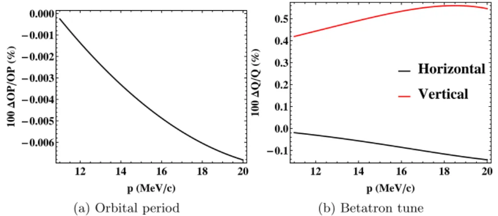
4.4.3 Betatron tune and chromaticity . . . 83
4.4.4 Orbital period . . . 94
4.4.5 Closed orbit position . . . 94
4.5 Further measurements from a decohering signal . . . 95
4.5.1 Finding the momentum distribution . . . 97
4.5.2 Measurement of the initial phase and lattice functions alpha and beta . . . 101
4.5.3 Simulation . . . 102
4.5.4 Momentum distribution measurement in EMMA . . . 105
4.5.5 Synchrotron radiation . . . 108
4.5.6 Transient beam loading . . . 109
4.5.7 Conclusions from lattice parameter reconstruction . . . 116
4.6 Amplitude dependent orbital period and tune . . . 117
4.6.1 Experimental method and results . . . 117
5 Synchrotron design study 123 5.1 The synchrotron lattice . . . 124
5.2 Tuning the lattice close to resonance . . . 125
5.3 Introduction of sextupole perturbations . . . 127
5.3.1 Chromatic and geometric effects of a sextupole pair . . . 128
5.3.2 Control of a separatrix through multiple sextupole pairs . . . 128
5.3.3 Theory of sextupole perturbations . . . 131
5.3.4 Off-momentum particles . . . 140
5.4 Final lattice parameters . . . 143
5.5 Transverse deflecting cavity . . . 147
5.6 Simulation of beam extraction . . . 149
5.6.1 Beam interrupt time . . . 149
5.6.2 Extraction with rf perturbation . . . 149
5.7 Summary and conclusions for the synchrotron design study . . . 158
6 FFAG Design Study 161 6.1 PAMELA . . . 161
6.2 Resonant extraction from the PAMELA lattice . . . 163
6.4 Dynamics of the half-integer resonant extraction process . . . 176 6.4.1 Flat top acceleration scheme . . . 178 6.5 Summary and conclusions for the FFAG design study . . . 178
7 Comparisons and Conclusions 183
7.1 Comparisons between synchrotrons and FFAGs for hadron therapy . . . . 183 7.2 Conclusions . . . 187
A Approximate model of an RF cavity 195
B EMMA modelling data 197
B.1 Quadrupole calibration . . . 197
Bibliography 205
List of Figures
1.1 Dose depth curves . . . 3
1.2 Proton range vs. kinetic energy . . . 4
1.3 Spread out Bragg peak . . . 6
1.4 Lawrence cyclotron . . . 8
1.5 Loma Linda synchrotron . . . 9
2.1 Particle motion in a uniform magnetic field . . . 15
2.2 Particle motion through uniform magnetic fields separated by drift spaces . . 16
2.3 Poincar´e plot . . . 17
2.4 Local coordinate system . . . 18
2.5 Multipole magnetic field profiles . . . 21
2.6 Multipole Lorentz force plot . . . 23
2.7 Scaling FFAG magnet field profile . . . 24
2.8 FODO cell stability . . . 26
2.9 Phase space ellipse (Courant-Snyder parameters) . . . 28
2.10 Betatron tune resonance diagram . . . 31
2.11 Transit time factor . . . 34
2.12 Longitudinal phase space portrait . . . 36
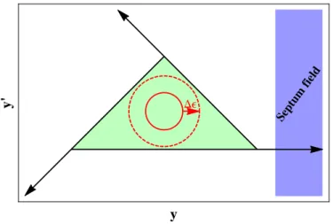
2.13 RF knockout phase space diagram . . . 37
2.14 Septum fields . . . 38
2.15 KEK radial sector FFAG . . . 40
2.16 PAMELA design concept . . . 43
2.17 PAMELA tune profiles . . . 43
2.18 Stability plot for FDF cell . . . 44
2.19 RACCAM lattice . . . 46
3.1 COSY/MAD/Zgoubi tracking comparison . . . 52
3.2 Charged particle motion in a magnetic field . . . 53
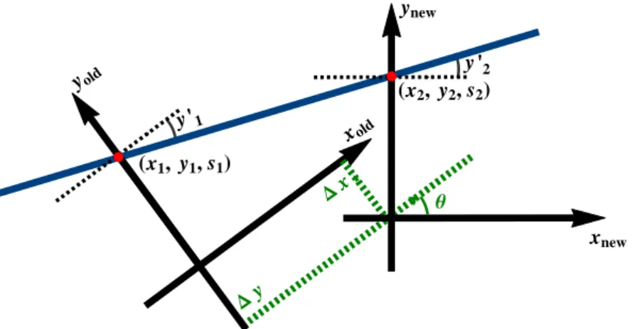
3.3 Reference axis transformation . . . 56
3.4 Convergence of tracking simulations (step length) . . . 58
3.5 Convergence of tracking simulations (integrator order) . . . 59
4.1 EMMA longitudinal phase space . . . 63
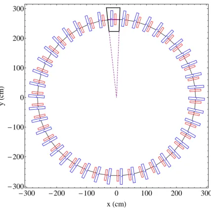
4.2 EMMA ring . . . 65
4.3 EMMA midplane field map . . . 66
4.4 EMMA periodic cell . . . 66
4.5 Overlap of EMMA field map . . . 67
4.6 Tune deviation in equivalent EMMA model . . . 68
4.10 EMMA quadrupole models (with field clamps) . . . 71
4.11 EMMA excitation curves . . . 72
4.12 EMMA field map/hard edge field comparison . . . 73
4.13 EMMA field dependence on longitudinal and transverse position . . . 74
4.14 Superposition of field maps . . . 75
4.15 Effect of using superposed maps on particle tracking . . . 76
4.16 Hard edge/field map closed orbit comparison . . . 76
4.17 Hard edge/field map orbital period comparison . . . 77
4.18 Hard edge/field map optical functions comparison . . . 77
4.19 Hard edge model optimisation results . . . 78
4.20 Tracking results for optimised hard edge EMMA models . . . 79
4.21 ALICE . . . 80
4.22 Excitation errors . . . 81
4.23 Equivalent momenta field profiles . . . 82
4.24 Real/equivalent momentum orbital period comparison . . . 82
4.25 Real/equivalent momentum tune comparison . . . 83
4.26 Example of EMMA BPM data . . . 84
4.27 Determination of betatron tune . . . 86
4.28 Tune calculation methods comparison . . . 87
4.29 Simulated BPM signal . . . 88
4.30 Tune calculation using decohering signal . . . 89
4.31 Tune calculation using signal with measurement errors . . . 90
4.32 Tune calculation for signal with both decoherence and measurement errors . 91 4.33 Tune calculation methods comparison for decohering beam and measurement errors . . . 91
4.34 Updated calculation of betatron tune . . . 92
4.35 EMMA experimental tune and field map tune. . . 92
4.36 Finding the chromaticity from measured tune data . . . 93
4.37 Finding the chromaticity with limited data points . . . 93
4.38 Measured EMMA orbital period . . . 94
4.39 Measured EMMA orbital period with field map orbital period . . . 95
4.40 Measured closed orbit position . . . 96
4.41 Decohering particle bunch . . . 98
4.42 Dependence of measured BPM signal on form of momentum distribution . . 99
4.43 Decoherence simulation result for a Gaussian momentum distribution . . . . 103
4.44 Effect of using limited BPM data to estimate the DTFT . . . 103 4.45 Convergence of momentum distribution reconstruction to a correct solution . 104 4.46 Convergence of momentum distribution reconstruction to a correct solution . 104
4.49 Fit of phase space ellipse to experimental data . . . 106
4.50 Convergence of experimental data . . . 108
4.51 Experimental indicators of beam loading . . . 109
4.52 EMMA orbital period with rf period . . . 113
4.53 Transient beam loading . . . 114
4.54 Simulated effects of beam loading on bunch centroid position . . . 115
4.55 Tune shift due to beam loading calculated from simulated BPM data . . . . 115
4.56 Convergence of betatron motion reconstruction based on simulated data with beam loading . . . 116
4.57 Measurements of vertical amplitude and β function vs. vertical corrector current in EMMA . . . 118
4.58 Vertical action dependence on vertical corrector current . . . 119
4.59 Orbital period dependence on vertical corrector current . . . 119
4.60 Orbital period dependence on vertical action . . . 120
4.61 Possible change in horizontal action during data collection for plot of orbital period vs. vertical action . . . 121
4.62 Measured amplitude detuning in EMMA . . . 121
5.1 Layout of the synchrotron lattice . . . 124
5.2 Synchrotron β functions . . . 125
5.3 Dispersion in synchrotron. . . 126
5.4 Synchrotron orbital period . . . 127
5.5 Synchrotron longitudinal phase space . . . 127
5.6 Synchrotron with single sextupole pair . . . 129
5.7 Chromaticity dependence on sextupole strength . . . 129
5.8 Comparison between separatrices formed by a single sextupole and a sex-tupole pair . . . 130
5.9 Separatrix rotation using two sextupole pairs . . . 130
5.10 Phase space plot stable particle bunch within separatrix . . . 131
5.11 Tune shift with initial start coordinate. . . 131
5.12 Diagram showing the location of the two sextupole pairs . . . 132
5.15 Separatrix rotation . . . 137
5.16 Separatrix orientation . . . 140
5.17 Momentum dependence of separatrix position . . . 141
5.18 Normalised dispersion . . . 143
5.19 Synchrotron with chromatic sextupoles. . . 144
5.20 Off-momentum separatrices for the revised extractions point . . . 144
5.21 Synchrotron separatrices during extraction . . . 145
5.22 Comparison between separatrices found theoretically and by tracking. . . 147
5.26 Plots to show the influence of a transverse rf perturbation on particles of
different initial action. . . 152
5.27 Extracted particles with initial transverse rf phase. . . 154
5.28 Extraction emittance and efficiency vs. septum position . . . 155
5.29 Extracted beam horizontal phase space vs. septum position. . . 156
5.30 Extracted particles with perturbation voltage. . . 157
5.31 Extracted particles with perturbation voltage. . . 158
6.1 Layout of the PAMELA proton ring . . . 163
6.2 Closed orbits in a single PAMELA cell . . . 164
6.3 Diagram showing a new PAMELA reference axis . . . 164
6.4 PAMELA Poincar´e portrait in horizontal phase space for 60, 120 and 230 MeV particles . . . 165
6.5 PAMELAβ functions . . . 165
6.6 PAMELA sextupole strength . . . 166
6.7 PAMELA decapole strength . . . 166
6.8 Tune footprint response to F/D ratio in PAMELA . . . 167
6.10 PAMELA vertical amplitude detuning . . . 168
6.12 Half-integer resonance without amplitude detuning . . . 171
6.13 Poincar´e plots for different tune distances from resonance. . . 172
6.15 PAMELA half-integer resonant extraction (tuning of resonant energy) . . . . 174
6.16 Input distribution of particles in vertical phase space. . . 175
6.17 PAMELA half-integer resonant extraction (mean extraction energy with standard deviation for four rates of acceleration). . . 175
6.18 PAMELA half-integer resonant extraction (extraction efficiency) . . . 176
6.19 PAMELA half-integer resonant extraction (effect of perturbation strength on mean extraction energy and efficiency). . . 177
6.20 Rate of amplitude growth when crossing half-integer resonance in PAMELA. 179 6.21 PAMELA half-integer resonant extraction (extraction efficiency when rf is switched off) . . . 180
6.22 Histogram showing extraction time profile for half-integer resonance crossing in PAMELA . . . 180
7.1 PAMELA acceleration time . . . 185
B.1 EMMA defocusing quad cross section . . . 197
B.2 EMMA defocusing quad field clamp cross section . . . 198
B.3 EMMA focusing quad cross section . . . 199
B.4 EMMA focusing quad field clamp cross section . . . 199
List of Tables
1.1 Accelerator related requirements of proton therapy. . . 7
2.1 Analytic expressions of multipole magnet field components. . . 21
2.2 Summary of the HIT synchrotron parameters. . . 39
2.3 Parameters of the radial sector scaling FFAG at KEK. . . 40
2.4 PAMELA proton lattice parameters. . . 42
2.5 Parameters for the RACCAM design. . . 46
4.1 EMMA DOFO cell parameters . . . 62
4.2 EMMA experimentally measured cell tunes . . . 90
4.3 α and β reconstructed using EMMA experimental data . . . 107
4.4 EMMA rf cavity. . . 113
5.1 Basic parameters of the proton synchrotron model. . . 128
5.2 Parameters of the synchrotron model (optimised for extraction) . . . 146
6.1 Table of lattice and cavity parameters for the PAMELA proton ring. . . 162
B.1 Profile of the defocusing pole tip from point A to B of Fig. B.1. . . 198
B.2 Profile of the defocusing quadrupole field clamp from point A to B of Fig. B.2.198 B.3 Profile of the focusing pole tip from point A to B of Fig. B.3. . . 200
B.4 Saturation curves for 1200-100A and 1006. . . 200
Accelerators play a key role in the delivery of radiotherapy for treatment of cancer and other medical conditions. Proton therapy has the benefit of more localised deliv-ery of dose to deep seated tumour volumes in comparison to treatment using x-rays or electrons. The accelerators currently used for proton therapy are cyclotrons and syn-chrotrons, which each have certain advantages and disadvantages. It has been proposed that accelerators of a fixed field alternating gradient (FFAG) design may combine some of the advantages and avoid some of the disadvantages of the existing machines. This thesis looks at the use of synchrotrons as a benchmark for the delivery of proton therapy, and then at how FFAGs may improve upon treatment delivery. Particular attention is paid to the beam dynamics issues, including comparisons between simulations and ex-perimental data taken with the EMMA non-scaling FFAG at Daresbury. The results of the comparisons show that simulation is able to predict the behaviour of a particle bunch in a real machine. The simulation tools are then used to evaluate the design of FFAGs incorporating resonant extraction techniques. In principle, resonant extrac-tion could overcome some problems of kicker based extracextrac-tion methods. The design study highlights technical challenges that would need to be overcome before resonant extraction could be implemented as a beneficial method for a proton therapy FFAG.
thesis
noun
1. A statement or theory that is put forward as a premise to be maintained or proved:
‘He vigorously defended his thesis on the causes of war.’
2. A penance for spending time doing research that you find interesting:
‘My thesis.’
I would like to thank the people who helped me create so much to write about, with special thanks to (in alphabetical order of first name) Andy Wolski, Bruno Muratori, David Kelliher, Kai Hock and Shinji Machida: you provided me with interesting chal-lenges, good guidance and the time needed to follow up ideas.
The Cockcroft Institute has always been a very welcoming environment; my time in office S30 would not have been the same without the many new friends that I have made whilst here. Thanks to you all.
Finally, but by no means with the least amount of gratitude, I must thank my family and friends. You made this possible.
Proton therapy and the role of
accelerators
1.1
Introduction
Particle accelerators are widely used for radiotherapy for the treatment of cancer. In 1957 a 3 GHz linear accelerator (linac) was used for the first time to produce a beam of x-rays to treat a patient with an ocular tumour [1]. In the years that have followed much research has gone into enabling treatments which deliver the maximum possible radiation damage to a tumour, whilst minimising damage to healthy tissue. This research has led to better imaging techniques for pinpointing and targeting tumours within the body, better understanding of how different biological tissues react to radiation (allowing clinicians to avoid unnecessary damage to radiosensitive organs) and better treatment techniques (such as the shaping of radiation beams to match the profile of a tumour). However, for most patients who receive radiotherapy, the treatment still means a beam of high energy x-rays delivered by a 3 GHz linac in a single room treatment facility. It may be a testament to the efficiency of linacs in producing treatment beams of electrons and x-rays, that, fundamentally, little has changed in terms of clinical accelerator technology since 1957.
In 1946 the potential therapeutic benefits of using protons rather than x-rays were described [2]. Since then the uptake of proton therapy has been slow, in part due to the technical challenges of delivering treatment beams of protons. In order to treat a tumour at a depth of 30 cm, protons with a kinetic energy of 230 MeV are needed (≈10 times higher than the electron energy required by conventional treatments). As a result, circular accelerators, which allow the accelerating rf structures to be reused a number of times per acceleration cycle, have become the preferred solution. The mass of the pro-ton, and limitations on the strength of magnetic fields that can be produced for steering a particle around a circular accelerator presently restrict just how compact these proton accelerators can be made. A hospital has to consider different factors depending on whether it wants to start offering proton treatments or treatments using electrons and
consists of several treatment rooms, each containing an electron linac. The operation of each linac does not depend on what is happening in other treatment rooms. A pro-ton based facility will also have several treatment rooms; however, due to the size and cost of the proton accelerator [3], one accelerator will typically serve all of the treatment rooms. The quality of treatment a proton therapy centre can offer is dependent upon the accelerator at its heart. To date, hospitals have used either a cyclotron or synchrotron accelerator, both of which offer distinct advantages and disadvantages. There is a de-mand for accelerator technologies that either help to make proton therapy more widely available, or improve upon the current standards of treatment. It has been proposed that accelerators of a fixed field alternating gradient (FFAG) design may be one way by which standards of treatment may be improved. This thesis evaluates the potential of FFAGs in the field of proton therapy, by making comparisons with the performance of a synchrotron accelerator.
1.2
Particles for cancer therapy
Late in the 19th century, shortly after R¨ontgen discovered x-rays, it was first observed
that radiation could have a damaging effect on tissue and that it could potentially be used in the treatment of cancer. Today it is understood that a successful radiation treatment means balancing the probability of controlling a tumour with the probability of causing the patient significant further harm due to a large exposure of healthy tissue to radiation. Careful choice of the particle used for radiotherapy is one of the ways through which the damage to a tumour can be maximised whilst minimising damage to healthy tissue. In evaluating the suitability of different particles for radiotherapy, it is often the relationship between absorbed dose and depth within water (a good approximation for tissue) that is considered. Here, the absorbed dose is the absorbed energy per unit mass and is measured in units of gray (Gy)[4]:
1 Gy = 1 J/kg.
1.2.1 Electrons and photons
a patient [5]. For treating deep-seated tumours, x-rays are the most commonly applied form of radiation. The notable features of the x-ray treatment are that the maximum dose occurs at a depth of several centimetres within the patient (with the depth of maximum dose increasing with beam energy), and that beyond the maximum dose, the dose then decreases exponentially with depth. As can be seen from Fig. 1.1, a potential problem with x-ray beam treatment is that, in the direction of the beam travel, the healthy tissue both before and after a tumour will receive a significant dose of radiation. The risk of complications from damage of normal tissue may be reduced by rotating the x-ray beam around a patient, whilst keeping the tumour volume at the axis of rotation, a process which reduces the maximum dose given to any one area of healthy tissue whilst maintaining a high dose within the tumour volume. However, in many cases, the ratio of the probability of eradicating a cancer to the probability of normal tissue complications (known as the therapeutic ratio) [6] may be improved through use of a different particle.
Figure 1.1: The relationship between the dose delivered to tissue and depth is depen-dent upon the particle used for therapy [7].
1.2.2 Protons and other hadrons
key advantage of using protons, or other ions (e.g. carbon ions), for therapy. The range
R(cm) of a proton in water is related to the proton kinetic energy Ek(MeV) by [8]:
R≈αEkp, (1.1)
whereα= 0.0022 cm MeV−p and p= 1.77.
100 150 200
0 5 10 15 20 25 30
Kinetic energyHMeVL
Range
H
cm
L
Figure 1.2: The approximate range (and hence Bragg peak depth) of a proton in water vs. proton kinetic energy calculated using Eq. 1.1. The energy of the proton
beam is selected so that the Bragg peak coincides with a tumour.
If the Bragg peak is positioned at a tissue depth corresponding to the location of a tumour, then a relatively low dose is received by the healthy tissue before the tumour and little or no1 dose after the tumour (Fig. 1.1). Having been proposed by Wilson in
1946, therapy based on use of the Bragg peak was first applied to a patient in 1960 [9]. For a treatment involving a beam of many particles, the width of the peak in the depth-dose plot depends on the type of charged particle used as well as the total range of the particles. The cause of this is range straggling, which is a result of the statistical variations in energy loss from each interaction of the treatment particle with the medium through which it is travelling. Range straggling means that each particle within a mono-energetic treatment beam will have a slightly different range. The range distribution is Gaussian, with a standard deviation approximately proportional to R/√A, where
R is the nominal range of the particle, and A the particle mass number [10]. Using heavier ions can lead to a sharper Bragg peak, however, the accelerators required tend to be larger and more expensive than for protons. In this thesis, emphasis is placed on accelerators for proton therapy, although some of the designs discussed are also capable of delivering heavier ions.
1Some dose is present beyond the Bragg peak due to neutron production and the additional range of
1.3
Beam requirements of proton therapy
Following diagnosis and an initial assessment of a tumour, a clinician will prescribe a radiation dose to the tumour volume. Typically this dose is measured in tens of gray, and is delivered in fractions of around 2 Gy per day over a number of weeks. Daily treatment times are minimised in order to maximize the patient throughput of a facility, and to reduce the error on dose distribution (which should not vary by more than±4 % throughout the tumour volume) due to patient movement; it is expected that the dose rate of a system should be at least 2 Gy/minute/litre which requires a beam current of approximately 0.5 nA [11].
The distal2 conformation of dose to a tumour is dependent upon the energy spread of the extracted beam as well as scattering in materials before the treatment volume. For a given treatment kinetic energy, Ek, the energy spread of the beam should be
less than ∆Ek/Ek = ±0.1 % at the point of extraction. The thin ‘pencil’-like beams
extracted from a proton accelerator typically have too small a cross sectional area and energy spread to deliver a uniform dose throughout an entire target tumour volume. Methods are required to spread the dose both laterally and longitudinally. The earliest treatments were based on a method known as passive scattering, whilst today, the best conformity of dose to a tumour volume is achieved using a method, first developed in the 1980’s, known as active scanning.
Passive scattering
Passive scattering uses a treatment field that is shaped to conform as closely as possible to the target tumour volume. To create the treatment field, scattering foils are used to enlarge the pencil beam [12, 13] followed by collimators to shape the enlarged beam so that it has the same lateral profile as the tumour [14]. To ensure that as uniform a dose as possible is delivered to the tumour longitudinally, a spread-out Bragg peak must be formed by delivering protons that have different ranges within a patient (Fig. 1.3) [15]. For a fixed energy particle source, the treatment beam is first passed through a range shifter, consisting of a perspex block with a thickness that positions the Bragg peak at the deepest point of the target volume. Following the range shifter, the beam is passed through a range modulator, which is often a rotating perspex disk of stepped thickness [16], to spread the Bragg peak longitudinally through the full depth of the treatment volume.
Passive scattering allows the required dose to be delivered to a tumour volume within a very short period of time, which has benefits in dealing with tumour movement re-sulting from, for example, respiratory cycles. However, the disadvantages of passive scattering include the spread out Bragg peak being of fixed width across the tumour volume and range straggling within the range shifter and modulator, both of which lead
Figure 1.3: The Bragg peak of a mono-energetic beam is typically too narrow to give a uniform dose throughout a tumour volume. A spread-out Bragg peak (SOBP) is produced by applying proton beams that have different ranges within the patient. The dashed blue line in the above plot shows the dose distribution calculated by summing the contributions from the individual Bragg peaks (solid blue lines) [17]. The contribution to the SOBP by the entrance dose of protons means fewer shorter range protons are
required than longer range protons in order to create a uniform dose distribution.
to a poorer conformation of dose to a tumour volume than is possible when using active scanning methods.
Active scanning
Table 1.1: Typical requirements of proton therapy affecting accelerator design (the energy step size and dynamic beam extraction intensity are based on the performance
of the Heidelberg Ion Therapy (HIT) synchrotron [26]).
Parameter Requirement
Extraction energy range 60-250 MeV Energy spread at extraction ∆Ek
Ek
±0.1%
Energy step size ∼0.7 MeV (1 mm steps) Energy switching time ≤1 s
Dose rate 2 Gy/min/litre
Dynamic beam extraction intensity 8×10⁷−2×10⁹pps
Stability at extraction point ±1 mm or±1 mrad
(where a beam is swept through the tumour volume in a very short period of time) and multi-painting (where the total dose is given to a tumour volume over several scans by the particle beam). These methods are discussed in more detail in chapter 6.
1.4
Accelerators for proton therapy
To date, the accelerators constructed for proton therapy have been either cyclotron or synchrotron circular accelerators [21]. Linear alternatives have been proposed [22], and ultra compact linear accelerators, which could, in future, see proton therapy centres based upon single room treatment facilities (resembling those offered by electron and x-ray therapy), are being investigated [23, 24]. It has been proposed that a circular accelerator of FFAG design may help to improve upon the quality of proton treatments currently available [25]. In this section, the basic features and principles of circular accelerators are described. Ultra compact linear accelerators are not discussed further, as they are considered to be beyond the scope of this study.
1.4.1 Cyclotrons
A simple cyclotron consists of two D-shaped electrodes within a dipole field (Fig. 1.4). Cyclotrons are well suited to a hospital environment due to their relatively compact size and simplicity.
Figure 1.4: Diagram of the Lawrence cyclotron in the plane of motion (left) and showing the magnetic fields between the poles of the Ds (right).
the gap between D’s. The acceleration cycle continues, with the path of the particle spiralling outwards as the number of interactions with the rf field increases. As the particle approaches the outer edge of the cyclotron, it is extracted. The acceleration process can be completed in approximately 10µs from injection to extraction. Good dynamic intensity control of the beam may be achieved by monitoring the extracted beam and then adjusting the ion source accordingly.
The rapid acceleration cycle of a cyclotron is a result of the fact that the magnetic fields and rf frequency can remain constant. The structure and operation of a cyclotron mean that the extracted beam has a fixed energy. In order to position the spread-out Bragg peak over the tumour volume, range shifters and modulators must be used. Although these methods allow for very rapid shifting of the position of the Bragg peak, they also introduce the problem of range straggling for lower energy treatments.
1.4.2 Synchrotron
Unlike the cyclotron, synchrotrons (such as the example shown in Fig. 1.5) confine particles to a single path. The layout of a synchrotron can be approximately described by a regular polygon. Dipole magnets are located at the vertices of the polygon in order to bend the particles around a closed circuit. In the straight sections between the dipoles, there are rf cavities for particle acceleration, as well as additional magnets which focus the beam, controlling the beam size and preventing particles from being lost on the walls of the accelerator.
During the acceleration process, the momentum of each particle will increase. In a uniform magnetic fieldB a particle with momentumpand chargeqwill follow a circular trajectory of radiusρ, where
Bρ= p
q. (1.2)
Figure 1.5: The synchrotron that is used to accelerate protons for therapy at the Loma Linda Medical Centre [27].
constant. Given the fixed path length, the time taken for a particle to make one rev-olution of the accelerator will change with the particle velocity during an acceleration cycle. Therefore, the frequency of the rf must also change to maintain synchronicity between the arrival of the particle bunch at a cavity and the desired phase of the rf.
A major advantage of the synchrotron for therapy is that the energy at which the particles are extracted can be varied easily from cycle to cycle, eliminating the need to degrade the beam by the use of range shifters and modulators. For treatments of tumours at small depths within a patient, this can mean better conformation of dose to a tumour volume than is the case when a cyclotron is used.
1.4.3 FFAG
In recent years, fixed field alternating gradient (FFAG) accelerators for hadron therapy have been the subject of a number of design studies [28–30]. It is claimed that accel-erators of this design have the potential to offer the benefits of both cyclotrons and synchrotrons, by giving:
- variable energy extraction;
- high repetition rate, leading to rapid dose delivery; - simple and stable operation due to fixed magnetic fields.
fields. FFAGs may be split into two categories, scaling and non-scaling. A scaling FFAG [31] has magnetic fields which vary radially within a plane according to:
Bz =Bz,0
R R0
k
. (1.3)
Here Bz,0 is the magnetic field perpendicular to the plane at a reference radius, R0,R
is the radial distance and k is known as the scaling index. The term ‘scaling’ refers to the fact that a high momentum particle will follow a path that is of the same shape but scaled up in size when compared to the path of a low momentum particle; the scaling index determines the proximity of the paths of particles at different momenta. Within a non-scaling FFAG, the field does not obey Eq. 1.3, and the shape of the path of a particle can vary with changing momentum. In both cases the magnetic field varies azimuthally so as to introduce alternating gradient focusing (alternating gradient schemes for FFAG accelerators are discussed further in chapter 2). For the scaling FFAG, the strength of the focusing is independent of the particle momentum, which ensures that the motion of the particles in the beam remains stable throughout an acceleration cycle. However, for the non-scaling FFAG, the strength of focusing can vary significantly with momentum (depending upon the field profile chosen) and there may be times during an acceleration cycle where, if the energy was fixed, the particle motion would be unstable. One advantage of the non-scaling FFAG is that it can be built using magnets that are less complicated than the magnets required for a scaling FFAG. The non-scaling FFAG also allows for the design of accelerators that have a reduced radial aperture and large acceptance when compared to a scaling FFAG (an accelerator with these qualities is discussed in chapter 4).
1.5
Thesis Overview
This thesis is organised as follows: - Chapter 1 introduces this thesis.
- Chapter 2 provides context by detailing an existing proton therapy facility as well as FFAG design concepts.
- Chapter 3 describes the tracking methods used for characterising the accelerators in computer simulations.
- Chapter 4 looks at the limitations of the design tools used in predicting particle behaviour in a given machine.
- Chapter 6 describes the FFAG design that will be discussed, and compared with the synchrotron design described in chapter 5.
Beam dynamics and accelerator
design
The momentum of a particle of charge q and velocity v travelling through electric (E) and magnetic (B) fields is influenced by the Lorentz force,
F= dp
dt =q(E+v×B), (2.1)
where p is the particle momentum as a function of time (t). This thesis will look at how particles are guided by magnetic fields and accelerated by electric fields within accelerators that deliver particle beams suitable for treating cancer. In this section, the physics of the relevant beam dynamics within accelerators will be introduced and given context through examples of existing accelerator designs.
2.1
Particles for acceleration
The charged particles encountered within the tracking studies in this thesis are electrons (chapter 4) and protons (chapters 5 and 6). The momentum of a particle is given by:
p=mv=γm0v,
withγ being the relativistic Lorentz factor and m0 the rest mass of the particle. When
defining the global properties of an electron beam within this thesis, the nominal mo-mentum of a single electron within the beam is given. This is in keeping with literature on the EMMA non-scaling FFAG (discussed in chapter 4), for which electrons are trav-elling at a speed greater than 0.99c. If the energy (E) of a particle is given by the rest energy (E0) and kinetic energy (Ek) of the particle:
E=E0+Ek,
E=mc2=γm0c2,
wherec is the speed of light. The kinetic energy of a particle can therefore be written:
Ek= (γ−1)m0c2.
When defining the global properties of a proton beam within this thesis, the nominal kinetic energy of a single proton within the beam is given. This follows the convention generally used in the literature on proton therapy. The energy, momentum and rest mass of a particle are related by:
E=p(pc)2+ (m 0c2)2.
The energy of particle beams are conventionally expressed in eV, which is the change in energy of an electron as it crosses a potential of 1 V. Particle momentum is given in units of eV/c and the mass in units of eV/c2. For ultra-relativistic particles, where
pc≫ mc2, values forE
k and pc approach that of E. When dealing with the dynamics
of particles within a bunch, it is often convenient to work with the momentum deviation of individual particles from a nominal momentum for the bunch. For both electrons and protons, the momentum of an individual particle within a beam is expressed as the fractional offset in its momentum (p) from the nominal momentum (p0),δ= p−p0p0 = ∆p0p.
2.2
Fundamentals of motion within a circular accelerator
Using a Cartesian coordinate system, a particle given some velocity in thezxplane will remain in the same plane and follow a circular path if there is a magnetic field directed along the y axis1. The radius of this path is given by,
ρ= p
qBy
. (2.2)
Figure 2.1 illustrates this case. A disc within the zx plane has been taken, within the disc there is a uniform magnetic field directed along the y axis. A charged particle given the appropriate starting conditions (position and velocity) will orbit around the centre of the disc (the path of such a particle is marked red in Fig. 2.1). Taking two more particles of the same energy, and giving one a slightly different starting velocity (Fig. 2.1a) and the second a different starting location (Fig. 2.1b), it is seen that the orbits of these two extra particles can be said to oscillate around the orbit of the original particle, but that in all cases each particle has the same location and velocity at the end of one orbit as it had at the start. The number of oscillations of a particle around the original path per orbit is called the betatron tune, which for pure dipole field is 1.
æ æ
æ æ
z
x
(a) Momentum offset from equi-librium orbit.
æ æ æ æ
z
x
(b) Spatial offset from equilib-rium orbit.
Figure 2.1: A particle with velocity in the zx plane travels on a disc that has a magnetic field directed along the y axis, the force experienced by the particle causes it to orbit around the centre of the plot (red path). If the initial velocity (blue path) or position (green path) of the particle is changed, then these new paths are seen to
oscillate around the original path.
The disc is now divided into quarters, and the quarters of the disc are moved outwards (as illustrated in Fig. 2.2) so that they are separated by regions with no magnetic field: these field free regions are referred to as drift spaces. Figure 2.2a shows a path for which a particle will have the same location and velocity at the end of an orbit as at the start; this path is referred to as the closed (or equilibrium) orbit. Particles following any other path are seen to oscillate around the closed orbit. However, unlike in Fig. 2.1, the particles do not return to their starting conditions after one orbit, but instead do so after three. The betatron tune in the case shown in Fig. 2.2 is 4/3.
These two examples are crude representations of the arrangement of magnets within a cyclotron (Fig. 2.1) and synchrotron (Fig. 2.2). For both arrangements, the return of the particles to their starting conditions after a given number of orbits is evidence of the focusing properties of a uniform magnetic field, there is clearly a range of initial conditions within the zxplane for which a particle will orbit indefinitely. The particle sources used for accelerators emit particles which have a spread of initial locations, ve-locities and energies; focusing methods are important in ensuring that as many particles as possible survive to the end of the acceleration cycle without being lost to the walls of the accelerator.
æ æ
z
x
(a) Equilibrium orbit.
æ æ
z
x
(b) Momentum offset from equi-librium orbit.
æ æ
z
x
(c) Spatial offset from equilib-rium orbit.
Figure 2.2: Separating the quadrants of the disc shown in Fig. 2.1 (with regions that have no fields) changes the particle dynamics. Figure (a) shows the equilibrium orbit for the new dipole configuration (this path is marked by the red dashed line in Figs. (b) and (c)); if particles have a momentum (Fig. (b)) or spatial (Fig. (c)) offset from the equilibrium orbit, then these particles will oscillate around the equilibrium orbit. In
this example the betatron tune is 4/3.
larger than 3 (Fig. 2.3b). The change in tune with the fractional offset in momentum is called the chromaticity. We now select an entrance plane to one of the dipole quarters as an observation point, and track a particle through 200 orbits in the disc. Each time the particle passes an observation point, its position and momentum along the x axis are recorded. Figure 2.3 shows that a plot of the recorded momentum vs. position forms an ellipse, at the centre of which is the closed orbit. The orientation of the ellipse in a plot of the transverse dynamical variables relative to the closed orbit is dependent upon where along the closed orbit the measurement is made; however, the area enclosed by the ellipse will remain constant (a matrix describing the propagation of the motion is symplectic).
æ æ æ æ
z
x
(a) Change in closed orbit with momentum.
æ æ
z
x
(b) Spatial offset from equilib-rium orbit.
æ
æ
æ
æ
æ
æ
æ
æ
æ
æ
æ æ
æ
æ æ
æ
æ æ
æ
æ æ
æ
æ
æ æ
æ æ
æ
æ æ
æ
æ æ
æ
æ æ
æ
æ æ
æ
æ æ
æ
æ æ
æ
æ æ
æ
æ æ
æ
æ æ
æ
æ æ
æ
æ æ
æ
æ æ
æ
æ æ
æ
æ æ
æ
æ æ
æ
æ æ
æ
æ æ
æ
æ
æ
æ
æ
æ
æ
æ
æ
æ
æ
æ
æ
æ
æ
æ
æ
æ
æ
æ
æ
æ
æ
æ
æ
æ
æ æ
æ
æ æ
æ
æ æ
æ
æ
æ æ
æ æ
æ
æ æ
æ
æ æ
æ
æ æ
æ
æ æ
æ
æ æ
æ
æ æ
æ
æ æ
æ
æ æ
æ
æ æ
æ
æ æ
æ
æ æ
æ
æ æ
æ
æ æ
æ
æ æ
æ
æ æ
æ
æ æ
æ
æ æ
æ
æ
æ
æ
æ
æ
æ
æ
æ
æ
æ
æ
æ
æ
æ
æ
æ
æ
æ
æ
æ
æ
æ
æ
æ
æ
æ æ
æ
æ æ
x
px
(c) Poincar´e plot.
Figure 2.3: The momentum of the particle in these plots is greater than that in Fig. 2.2. Dispersion leads to a closed orbit that is found at a larger radius: the closed orbit for the new and previous momenta are shown by the solid and dashed red lines in Fig. (a) respectively. Figure (b) shows that the path of a particle that is offset from the equilibrium orbit no longer closes every three turns; the change in betatron tune with a fractional change in momentum is called the chromaticity. A particle is tracked through 200 turns, and the phase space variables, position and momentum, of the particle in the direction of thexaxis are recorded at a boundary of the lower right quadrant (marked orange in Fig. (c)); the plot of px vs.x at the boundary traces out an ellipse. If the
x
s
z
y
machine centre
Figure 2.4: Coordinate system local to the equilibrium path of a particle beam. x
is the longitudinal coordinate (tangential to the closed orbit). y andz are transverse horizontal and vertical respectively.
accelerated the increase in velocity is compensated by the increase in orbital circumfer-ence, so the orbital period remains constant. However, in a synchrotron, the fields are ramped up during acceleration so as to overcome the effect of dispersion and maintain a fixed closed orbit. In FFAGs, the magnetic fields increase with radius, which results in a reduction of the dispersion. For both synchrotrons and FFAGs the motion of particles can be described in terms of small oscillations (compared to the orbital radius) around closed orbits: for this reason it is convenient to use a coordinate system that has an origin at or close to the position of the closed orbit of a beam at any point around the circumference of the accelerator (Fig. 2.4).
The focusing provided by a uniform field directed along theyaxis acts only in thezx
plane. Eventually, any particle with some component of velocity in the y direction will be lost. A number of non-uniform field profiles (introduced in section 2.3) are commonly applied in accelerators to provide both horizontal and vertical focusing and to ensure that the beam dynamics within an accelerator are as required for any given application.
2.3
Magnets for accelerators
In section 2.2, we demonstrated that a uniform magnetic field could have a focusing effect of the motion of a charged particle. The focusing was limited to constraining particles along an axis that was perpendicular to both the magnetic field and the direc-tion of modirec-tion of a particle travelling along the closed orbit (the transverse horizontal
when chromaticity was introduced; later in this chapter we will see why we may want to control the chromaticity of a lattice, and how this can be achieved using a variety of magnetic field profiles.
An understanding of the magnetic field profiles that can be produced for use within a particle accelerator can be gained by starting with two of Maxwell’s equations,
∇ ×H= ∂D
∂t +J, (2.3)
∇ ·B= 0, (2.4)
whereB=µ0H, withµ0being the permeability of free space,Dthe electric displacement
and Jthe current density. In the vacuum of a beamline that is surrounded by magnets and zero (or constant) electric fields, Eq. 2.3 may be rewritten as
∇ ×H= 0. (2.5)
It follows that we can write the magnetic field in terms of a magnetic scalar potential,
ψ:
B=−∇ψ. (2.6)
Combining Eq. 2.4 and Eq. 2.6 then gives Laplace’s equation for the scalar potential,ψ: ∇2ψ= 0. We consider the case where magnetic fields vary along the transverse axes of a
magnet, but are constant along the longitudinal axis. This can be a good representation of the fields within a magnet when away from the entrance and exit, in which regions the fields do not vary with longitudinal position. Restricting this derivation to two dimensions, Laplace’s equation in polar coordinates has the form:
∇2ψ= ∂
2ψ
∂r2 +
1
r ∂ψ
∂r +
1
r2
∂2ψ
∂φ2 = 0, (2.7)
where, based on the local coordinate system of Fig. 2.4, r = py2+z2 and φ =
arctanzy. A solution to Eq. 2.7 is given by [32]:
ψ=
∞
X
n=1
(anrncos(nφ) +bnrnsin(nφ)), (2.8)
where, in the case of a pure multipole field, 2nis the number of magnet poles. The an
and bn coefficients determine the field strengths of the cosine and sine terms which are
at an angle of π/2n (skew multipole) and normal (upright multipole) to the xy plane respectively. Taking the normal quadrupole as an example, n = 2 and a2 = 0, then
Eq. 2.8 evaluates to:
ψ2 = 2b2yz. (2.9)
The magnetic field is then found by using Eqs. 2.6 and 2.9:
B=−2b2(z, y,0),
which may be written in terms of the field gradient along an axis in the quadrupole:
B= ∂By
∂z (z, y,0).
The Lorentz force on a particle travelling perpendicular to the longitudinal axis of the quadrupole (v= (0,0, vx)) is:
F=qvx
∂By
∂z (z,−y,0).
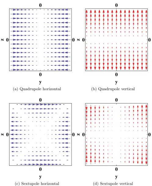
At this point we note that the force along the horizontal and vertical transverse axes of the normal quadrupole are dependent on z and −y respectively. This property makes the quadrupole focusing for one transverse axis and defocusing for the other. In section 2.4 we see how pairs of quadrupole magnets are used to provide focusing along both transverse axes. The accelerators within this thesis are constructed with upright multi-pole magnets; however, in practice, there will be small skew multimulti-pole field components due to errors in the rotational alignment of magnets. Equation 2.8 has been evaluated for the first four values of n, with the results in Cartesian coordinates of the upright multipole fields given in table 2.1 and the field profiles shown in Fig 2.5. Figure 2.6 shows the force experienced by a particle as it passes through a quadrupole magnet and through a sextupole magnet, as a function of transverse position in the magnet. Throughout this thesis, we define multipole magnets by their normalised gradient (or strength), which is given by:
Kn−1 =
∂n−1B
y
∂zn−1
1
Bρ, (2.10)
where Bρ is referred to as the particle rigidity, and relates the magnetic field (B) and bending radius (ρ) experienced by a particle to the particle momentum (p) and charge (q):
Bρ= p
q. (2.11)
Table 2.1: Analytic expressions of multipole magnet field components.
Component By Bz
Dipole 0 BρK0
Quadrupole BρK1z BρK1y
Sextupole BρK2yz 12BρK2(y2−z2)
Octupole 16BρK3(3y2z−z3) 16BρK3(y3−3yz2)
y
z
(a) Dipole
y
z
(b) Quadrupole
y
z
(c) Sextupole
y
z
(d) Octupole
Figure 2.5: Field profiles for the first four multipole magnet components. With the defined coordinate system, particles travel out of the page; the quadrupole field shown will be horizontally focusing for a negatively charged particle, and defocusing for a
Bz =Bz,0
R R0
k
=Bz,0
1 +k∆R
R0
+(k−1)k∆R
2
2R2 0
+(k−2)(k−1)k∆R
3
6R3 0
+...
=Bz,0 1 +
∞
X
n=1
k(k−1)(k−2)...(k−n+ 1)∆Rn n!Rn
0
!
,
(2.12)
whereR=R0+ ∆R. Figure 2.7 shows the field profile that satisfies the first 5 terms of
Eq. 2.12, which, for the range shown, is a good approximation for the scaling FFAG mag-net. Later in this chapter, two FFAG accelerator designs are discussed: one is built using scaling FFAG magnets; the second is designed with combined function magnets (where the fields within an accelerator magnet consist of two or more multipole components) that satisfy the first 5 terms of Eq. 2.12.
2.4
Linear particle dynamics
Understanding the motion of a particle with respect to the closed orbit can give key information about the performance of a particle accelerator. A popular approach is to describe each accelerator component in terms of a Hamiltonian that determines the dynamics of a charged particle within the component. From this, Hamiltonian maps that propagate the dynamical variables through the different accelerator components can be derived. The coefficients within these maps tell us about the behaviour of a particle beam at the location of the corresponding component within the accelerator. Maps for a sequence of components can be combined to produce a map for some section of accelerator, or even for an entire accelerator. The particle tracking studies within this thesis have been carried out using numerical methods (which are discussed in chapter 3), the results of tracking are often then used to calculate the map that describes the linear particle motion through the accelerator.
In Fig. 2.4 a coordinate system local to the closed orbit of a particle was defined. The transverse motion of a particle with respect to the closed orbit may be described by using the dynamical variablesy, y′, zandz′, where the prime indicates the change in a variable with respect to the path length, s, of a particle following the closed orbit; the value of y′, for example, can be calculated as:
y′ = arctan
py
px
,
where py is transverse horizontal momentum with respect to the closed orbit and px is
the momentum tangential to the closed orbit at a given location.
0 0
0
0
y
z
(a) Quadrupole horizontal
0 0
0
0
y
z
(b) Quadrupole vertical
0 0
0
0
y
z
(c) Sextupole horizontal
0 0
0
0
y
z
(d) Sextupole vertical
Figure 2.6: Horizontal and vertical forces experienced by a charged particle travelling through a magnetic multipole field.
y
z
Figure 2.7: Field profile of a combined function magnet containing components from dipole up to decapole. This is approximately equivalent to a scaling FFAG magnet over
the range shown.
equations, which are known as Hill’s equations:
∂2y
∂s2 +Ky(s)y= 0,
∂2z
∂s2 +Kz(s)z= 0, (2.13)
where the functionsKy(s) and Kz(s) are the piecewise constants that give respectively
the transverse horizontal and vertical focusing strength of a component at a position
s. In a circular accelerator, a particle will encounter the different steering and focusing components once every turn in the accelerator, so that along the horizontal axis, for example, Ky(s) = Ky(s+C), where C is the path length of a particle following the
closed orbit for one turn. If steering occurs only in the xy plane, then the horizontal and vertical focusing functions at a given position, s, are written as:
Ky =
1
ρ(s)2 +K1(s), Kz =−K1(s), (2.14)
where ρ is the bending radius of a dipole magnetic field component and K1 is the
quadrupole magnet focusing strength that was defined in section 2.3. A solution to Hill’s equation for positive values ofK is given by [33]:
y(s) =acos (pKys+b), (2.15)
whereaandbare determined by the initial phase space coordinates of a particle (y0, y′0).
Through expansion of the cosine term of Eq. 2.15, we can write:
y(s) =Acos (p
Kys) +Bsin (
p
and then by differentiatingy with respect to s, we obtain an expression for y′:
y′(s) =−p
KyAsin (
p
Kys) +
√
KBcos (p
Kys).
If we take the limit of s→0, we find thatA =y0 and B =y0′/ p
Ky, and we can now
write the transfer map for propagating the dynamical variables through a combined function dipole (with horizontally focusing quadrupole terms, Ky >0) of length,L:
Mf=
cos p
KyL √1K
ysin
p
KyL 0 0
−p
Kysin pKyL cos pKyL 0 0
0 0 coshp
|Kz|L
1 √
|Kz|sinh
p
|Kz|L
0 0 p
|Kz|sinh
p
|Kz|L
coshp
|Kz|L
(2.16)
To find the dynamical variables after the component, we then multiply the map by the initial dynamical variables:
y1
y′
1
z1
z′
1
=Mf
y0
y′
0
z0
z′
0
.
The transfer matrix, Mf, contains both ordinary and hyperbolic trigonometric terms;
this provides a description of the focusing action of the quadrupole along the horizontal axis and defocusing along the vertical axis. In the case that Ky < 0, we refer to the
quadrupole as being defocusing, and the map is given by:
Md=
cosh p
|Ky|L √|1K
y| sinh p
|Ky|L 0 0
p
|Ky|sinh p|Ky|L cosh p|Ky|L 0 0
0 0 cos √KzL √1Kzsin √KzL
0 0 −√Kzsin √KzL cos √KzL
.(2.17)
It is possible to have a net beam focusing effect along both transverse axes by con-structing accelerator lattices with sequences of focusing and defocusing quadrupoles that are separated by drift spaces. The FODO (focusing-drift-defocusing-drift) cell is a common example; we can calculate a map for transporting particles through a FODO cell by multiplying the maps for the individual components together in the following fashion:
M =MoMdMoMf, (2.18)
where Mo is the map for a drift space. The quadrupole maps given describe motion

![Figure 1.5: The synchrotron that is used to accelerate protons for therapy at the Loma Linda Medical Centre [27].](https://thumb-us.123doks.com/thumbv2/123dok_us/8070078.226818/25.892.287.659.117.497/figure-synchrotron-accelerate-protons-therapy-linda-medical-centre.webp)