Improving Closed Loop Signal Shaping of Flexible Systems with Smith Predictor and Quantitative Feedback

Article

Improving Closed-Loop Signal Shaping of Flexible

Systems with Smith Predictor and Quantitative

Feedback

Withit Chatlatanagulchai

a,

_*

_{, Puwadon Poedaeng}

b

_{, and Nitirong Pongpanich}

c

Control of Robot and Vibration Laboratory, Department of Mechanical Engineering, Faculty of

Engineering, Kasetsart University, 50 Ngam Wong Wan Rd, Lat Yao, Chatuchak, Bangkok 10900, Thailand E-mail: a_{fengwtc@ku.ac.th (Corresponding author),} b_{moopuwadon@hotmail.com,} c_{aook-aik@hotmail.com}

Abstract. Input shaping is a technique used to move flexible systems from pointtopoint rapidly by suppressing the residual vibration at the destination. The vibration suppression is obtained from the principle of destruction of impulse responses. The input shaper, when placed before the flexible system inside the control loop, proves to deliver several benefits. However, this so-called closed-loop signal shaping has one major disadvantage that it adds time delays to the closed-loop system. Being a transcendental function, the time delays cause difficulty in analysis and design of the feedback controller. In most cases, the time delays also limit the maximum achievable bandwidth. In this paper, for the very first time, Smith predictors were applied to the closed-loop signal shaping to remove the time delay from the loop. It was shown in simulation result that the detrimental effect of the time delays was completely removed in the case of perfect plant model. The quantitative feedback control was used in the study to quantify the amount of achievable bandwidth and to suppress vibrations from the plant-input disturbance.

Keywords: Smith predictor, input shaping, closed-loop signal shaping, vibration suppression, quantitative feedback.

ENGINEERING JOURNAL Volume 20 Issue 5 Received 27 December 2015

1.

Introduction

Flexible systems, when moved from point to point rapidly, exhibit residual vibration at their destination. Input shaping technique suppresses this residual vibration by superposition and cancellation of impulse responses. Impulse sequence is formed as an input shaping filter and implemented as an FIR filter. The amplitudes and time locations of the impulses are computed to obtain complete cancellation of impulse responses. The input shaping technique was originally proposed by Smith in [1] under the name Posicast control. It was later made more robust to uncertainty in the mode parameters by Singer and Seering in [2] and was given the name Input shaping.

Since its origin in the 50’s, the input shaping technique has found numerous applications with flexible systems. Cranes are among the most popular applications of the input shaping technique due to the requirement to suppress payload swing. Notable literature includes those of gantry crane [3], bridge crane [4], tower crane [5], and boom crane [6]. Robot manipulators have flexibility in their joints and links that have to be taken into account during the design. Literature includes those of flexible-link robot [7] and flexible-joint robot [8]. Input shaping has also been used in suppressing the liquid sloshing in container [9], suppressing vibration of the flexible appendages of the flexible spacecraft [10], suppressing probe vibration in coordinate measuring machine (CMM) [11], designing cam profile that reduces vibration of the cam-follower system [12], reducing vibrations during small motion and unloading operations of a telescopic handler [13], suppressing vibration in a cherry picker due to its flexible joints [14], suppressing the oscillatory transients in a dual-solenoid positioning servo actuator [15], and eliminating bouncing in a micro-electro-mechanical-system (MEMS) contact switch [16].

The input shaping filter can be placed either outside the loop or inside the loop. Outside-the-loop input shaping filter is designed from the mode parameters (natural frequency and damping ratio) of the closed-loop system. It can only suppress vibration from the reference signal. However, there is no detrimental effect from the time delay of the input shaper because the input shaper is placed outside the loop. When the input shaper is placed inside the loop before the flexible plant, so-called closed-loop signal shaping (CLSS) [17], the input shaper is designed from the mode parameters of the flexible plant.

The CLSS offers several advantages over the outside-the-loop input shaping because, in CLSS, the input shaping filter becomes a part of the closed-loop system. First, CLSS can suppress the vibrations induced by the reference signal, the plant-output disturbance, and noise. Second, CLSS can easily be designed for flexible plants that have hard nonlinearities. The hard nonlinearities, such as actuator saturation, deadzone, and backlash, can modify the input-shaped command thus reduce its vibration-reducing performance. In CLSS, the input shaper is placed directly before the hard nonlinearities; therefore, it is easy to design the input shaper such that its input-shaped command will not be modified by the hard nonlinearities. Third, CLSS can be used to greatly improve control performance of the human operator, performing manual control of the flexible system. In manual control, the human operator is the feedback controller. It was shown by Potter and Singhose in [18] that human can control the flexible system better when there is an input shaper placed in front of the flexible system to reduce its vibration.

Nevertheless, because the input shaper contains time-delay terms, the CLSS bring the time delay into the closed-loop system, which is the major disadvantage of the CLSS. The closed-loop characteristic equation of the system with CLSS possesses exponential time-delay function. Since the exponential function is transcendental, it is difficult to analyze the stability property or to design a controller for the system. For example, Huey and Singhose [19] showed that, with CLSS, there are infinitely many root locus branches. Only in simple cases, a finite number of root locus branches closest to the real axis can be used in stability analysis. From the root locus stability analysis, Huey and Singhose [19] pointed out that CLSS requires quite an accurate plant model to avoid unexpected instability. Huey and Singhose [20] showed that CLSS cannot suppress the vibration induced by the plant-input disturbance or by non-zero initial conditions. Moreover, it is a well-known fact [21] that time delay in the loop can limit the maximum achievable bandwidth and phase margin and; therefore, limit the performance of the control system.

characteristic equation can affect the stability. Second, if the process has an integrator (as is normally the case of the flexible system), a constant plant-input disturbance may result in non-zero steady-state tracking error. Both disadvantages will be investigated in this paper.

The Smith predictor was applied to the CLSS in our pioneering work [23]. This paper expands on the work in [23], yet it still remains one of the very first work that proposes this idea. Robust stability and robust performance (the case when the plant model differs from the actual plant) of the proposed technique is explored in this paper. When the plant model differs from the actual plant, unexpected result such as instability may occur from using Smith predictor, depending on the type of plant and controller.

In this paper, classical Smith predictor was applied to the CLSS. The quantitative feedback control [24] was used as the primary feedback controller. The paper offers the following advantages over the existing CLSS:

 The Smith predictor removes the time delay of the input shaper from the characteristic equation. As a result, the feedback controller can be designed as if the time delay was not present.

 To avoid unexpected instability caused by the CLSS when the plant model is uncertain, a quantitative feedback control was used to ensure stability for all expected plant uncertainties.  The quantitative feedback control was used to reject the vibration induced by the plant-input

disturbance or by non-zero initial conditions.

 All the advantages of the CLSS are still preserved with the proposed technique.

This paper is organized in the following way. Section 2 introduces the input shaping technique, the classical CLSS, the CLSS with classical Smith predictor, and the flexible system with one flexible mode that will be used in simulation. Section 3 contains the CLSS with Smith predictor and quantitative feedback control, together with simulation result. Section 4 presents conclusions and future work.

2.

Closed-Loop Signal Shaping with Smith Predictor

2.1. Input Shaping

A floating oscillator plant with transfer function

 

2 2 2,

2

n

n n

P s

s s



 



  (1)

where n is the natural frequency and  is the damping ratio, has two oscillatory poles at

1,2 n d,

s   j where ₁ 2

d n

   is the damped natural frequency. A zero-vibration (ZV) input shaper [2] has transfer function

 

2

1 2 ,

t s ZV

IS s A A e (2)

where A11 / 1



K



, A2K/ 1



K



, t2 / d,





2

exp / 1 .

K   It is easy to show that

 

1,2 0,

ZV

IS s  which means that the input shaper uses its zeros to cancel the plant’s two oscillatory poles

to remove the vibratory mode from the system, resulting in zero residual vibration. In fact, the input shaper (2) has infinitely many zeros, as can be shown by setting 2 

1 2 0,

t j

AA e    resulting in   _n and

, 1, 3, 5, ...

d

k k

    . Note that the pair of input shaper’s zeros that is the closest to the real axis is used to cancel the plant’s two oscillatory poles, yielding the shortest input shaper duration t2.

It can be seen that the input shaper (2) requires the knowledge of the mode parameters n and . For more robustness to parameter uncertainty, multiple zeros of the input shaper can be placed over the plant’s oscillatory poles, leading to the so-called zero-vibration-and-derivative (ZVDk_{) input shaper with transfer}

functions

 



2



1

1 2 , 1, 2, 3, ...

k t s ZVDk

2.2. Classical CLSS

Consider the classical closed-loop signal shaping [17] as shown in Fig. 1. P represents a flexible system,

whose transfer function is

 

n

 

/ d

 

,

P s P s P s

where Pn and Pd are the numerator and denominator of P. IS is the input shaper. C represents a primary controller. NL represents the hard nonlinearities. r is the reference signal; u is the control effort;

I

d is the plant-input disturbance; dO is the plant-output disturbance; n is the noise, and y is the output of interest.

Fig. 1. Classical closed-loop signal shaping.

The closed-loop transfer functions from each external signal to the output y of the CLSS in Fig. 1 are

 

     

_{       }

_{       }

 

_{       }

     

 

       

 

       

 

 

       

 

1

1 1 1

.

I O

n n d

I O

d n d n d n

P s IS s C s P s

y s r s d s d s

P s IS s C s P s IS s C s P s IS s C s

P s IS s C s P s P s

r s d s d s

P s P s IS s C s P s P s IS s C s P s P s IS s C s

  

  

  

  

(3)

By inspecting the transfer functions above, the first advantage of the CLSS that it can suppress the vibrations induced by r d, _O, and n can be stated. P sd

 

contains oscillatory poles of the flexible plant

 

P s ; therefore, the oscillatory poles are also the poles of the closed-loop transfer functions. For the

closed-loop transfer function from r to y, the zeros of IS s

 

are designed to cancel with those of P sd

 

,

so the vibration induced by r is suppressed. For the closed-loop transfer function from d_O to y, the

zeros of P sd

 

cancel with the oscillatory poles of the plant, so the vibration induced by dO is also suppressed. The transfer function from n to y is merely the negative of that from r to y; hence, the

vibration induced by the noise n can also be suppressed. The second advantage of the CLSS that it can

easily be designed for flexible plants with hard nonlinearities can be explained by inspecting the CLSS diagram in Fig. 1. The hard nonlinearity, NL, can be actuator saturation, deadzone, or backlash. NL

changes the shaped signal coming out of the input shaper, IS, so the performance of the input shaper is

degraded. With the CLSS, an inverse of the nonlinearity, NL, can be placed before the input shaper, IS, so

the shaped output coming out of the input shaper will not be altered by the nonlinearity, NL; therefore, the

performance degradation can be avoided. The third advantage of the CLSS that it can be used to improve human control of the flexible system can also be shown by inspecting the CLSS diagram in Fig. 1. In manual control, human is used as the primary controller, C, with eyes aiming at the output, y, of the

flexible plant and hand gives the control effort, u. With CLSS, where an input shaper, IS, is placed before

the flexible plant, P, the output, y, will not oscillate; hence, the human control performance is improved.

This result was confirmed in [18].

The first disadvantage of the CLSS is that it cannot be used to suppress the vibration induced by the plant-input disturbance, dI. This fact can be seen from the closed-loop transfer function from dI to y.

P IS

C

I

d

r

-u y

O

d

[image:4.595.162.430.254.334.2]

The zeros of P sn

 

do not cancel with those of P sd

 

. Because non-zero initial conditions can be thought of as a plant-input disturbance [25], the CLSS cannot suppress the vibration induced by the non-zero initial conditions as well. The second disadvantage of the CLSS comes from the time-delay term in the input shaper (2). From Eq. (3), the transfer function of the input shaper, IS, appears in the denominator of the

closed-loop transfer functions. Because the time-delay term, _et s2 _, is a transcendental function of _s,

conventional control design and stability analysis do not apply. Some rational-function approximation (e.g. Pade approximation) of the time-delay term must be applied, introducing additional uncertainty into the system. Moreover, the time-delay term in the CLSS results in non-minimum phase system which, according to [21], limits the performance of the control system by limiting the maximum achievable bandwidth. The third disadvantage of the CLSS was pointed out by Huey and Singhose [19] that the CLSS requires accurate plant model in order to avoid unexpected instability.

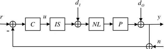
2.3. CLSS with Classical Smith Predictor

Consider the CLSS with the classical Smith predictor as shown in Fig. 2. The classical Smith predictor,

,

SM has a transfer function

 

 

   

.

SM s P s P s IS s (4)

Fig. 2. Closed-loop signal shaping with classical Smith predictor.

The closed-loop transfer functions from r and dI to y can be computed as

 

     

_{     }

 

1

     

_{   }

 

.

1 1 I

C s IS s P s C s IS s P s

y s r s P s d s

C s P s C s P s

 

 _  _  _ _

  (5)

Comparing Eq. (5) to Eq. (3), the transfer function of the input shaper, IS, is no longer present in the

denominator of the closed-loop transfer functions. As a result, conventional control design and stability analysis can be applied to the closed-loop system.

There are two disadvantages of the system in Fig. 2. First, when the actual plant, P, and its model, Pˆ,

are different, the closed-loop transfer functions from r and dI to y become

 

     

   

     

     

 

 



   

     



   

     

     

 

ˆ ˆ

1

ˆ ˆ

1

.

ˆ ˆ

1 I

C s IS s P s

y s r s

C s P s C s P s IS s C s IS s P s

P s C s P s C s P s IS s

d s C s P s C s P s IS s C s IS s P s 

  

 



  

(6)

It can be seen that when the plant uncertainty exists, the time delay from the input shaper, IS, is not

removed in its totality from the denominator of the closed-loop transfer function and therefore still affects the control system. Second, if the disturbance, dI, is present, the steady-state tracking error may not be

zero.

P IS

C

SM

I

d

r

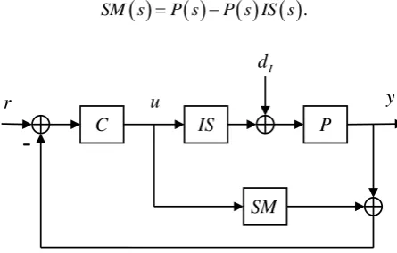
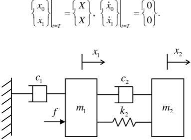
[image:5.595.181.404.302.444.2]

2.4. Flexible System with One Flexible Mode

As an example, consider a flexible system with one flexible mode as shown in Fig. 3. In general, the system represents two entities, connected via a flexible part, which encompasses a large majority of actual rigid-flexible systems. The driving one has an absolute position and mass of x1 and m1, and the driven one has

2

x and m₂. k c₂, ₁, and c₂ are spring stiffness and two damping constants. f is the control force. The

objective is to move both masses from the origin to a displacement X with zero residual vibrations and in

a shortest time possible T, that is,

0 0

1 1

0

, .

0

t T t T

x X x

x _ X x _

       

 

       

   

   

Fig. 3. Flexible system with one flexible mode.

The transfer function from f s

 

to x2

 

s is given by

 



2



2





3 2

1 2 1 2 2 2 2 1 1 2 2 2 2 1 1 2

.

c s k P s

s m m s m c m c m c s m k m k c c s c k 



        

  (7)

For simplicity, the ZV input shaper (2) and a PI controller,

 

1

1 ,

p i

C s K

T s

 

 _  _

  (8)

where Kp and Ti are controller gains, are considered.

For simulation purpose, let c150 kg/s, c20.1 kg/s, m11 kg, m22 kg, and

2

2 8 kg/s .

k  The plant

(7) has one flexible mode with  _n 2 rad/s and  0.05. The ZV input shaper (2) has the impulse

amplitudes A10.541 and A20.459 and the time location t21.572 s. The PI controller (8) was designed

as Kp 10 and Ti 20.

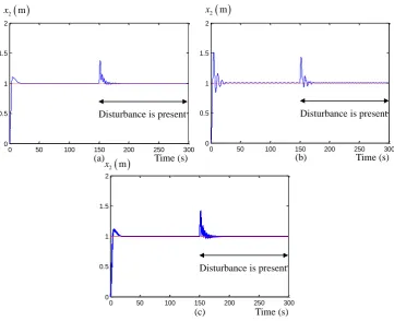
The reference, r, is a unit-step signal, and there exists a step plant-input disturbance, dI, of magnitude

10 during 150th _{to 300}th _{seconds. Figure 4 shows the tracking result where the dash lines are the reference}

signal and the solid lines are the output, yx2, signal. Figure 4(a) shows the case without using the input

shaper. The output is vibrating. Figure 4(b) shows the case when the CLSS with classical Smith predictor (4) was implemented. The input shaper in the CLSS setting suppresses most of the vibration from the reference signal. However, it cannot suppress the vibration induced by the plant-input disturbance. Moreover, it is a well-known result that the classical Smith predictor yields non-zero steady-state tracking error when disturbance is present (Section 9.8 of [26]).

1

c

2

m

1

x x2

2

c

2

k

1

[image:6.595.199.391.200.341.2]

Fig. 4. Tracking result. (a) Without input shaper. (b) Use CLSS with classical Smith predictor as shown in Fig. 2. Dash lines are the reference signal; Solid lines are the output yx2.

To cope with the non-zero tracking error due to the disturbance, many researchers have already proposed the modifications to the classical Smith predictor. See, for example, two classical works by Watanabe and Ito [27] and Astrom et al. [28], a two degrees-of-freedom method by Normey-Rico and Camacho [29], and a recent publication by [30].

This paper applies a scheme, called feedforward Smith predictor [31], to eliminate non-zero tracking error due to the disturbance. In this scheme, the disturbance, dI, is measured and is fed to the Smith predictor.

By doing so, the effect of the disturbance is counteracted before it can change the output.

Our method is based on the quantitative feedback control [24]. The two disadvantages from using the classical Smith predictor, namely the uncertainty in the plant model causing unexpected performance degradation and the non-zero steady-state tracking error under the presence of the disturbance, will be considered.

[image:7.595.104.494.80.238.2]

3.

CLSS with Smith Predictor and Quantitative Feedback

Figure 5 shows the proposed system. The input shaper, IS, is designed to suppress the vibration mode of

the flexible plant, P. The classical Smith predictor, SM, removes the time delay of the input shaper from

the loop so that conventional feedback control design can be applied. The feedback controller, C,

attenuates the effect of the disturbance, dI, and ensures closed-loop stability. The controller, C, together

with the pre-filter, F, enables good tracking performance. The disturbance, dI, is measured and fed to the

Smith predictor to eliminate non-zero tracking error due to the presence of the disturbance.

Fig. 5. CLSS with classical Smith predictor and quantitative feedback control.

Suppose the actual plant, P, and its model, Pˆ, are different by a multiplicative uncertainty, given by





ˆ 1 _m ,

PP   (9)

Time (s) (a)

 

2 m

x

Time (s) (b)

 

2 m

x

0 50 100 150 200 250 300

0 0.5 1 1.5 2

0 50 100 150 200 250 300

0 0.5 1 1.5 2

Vibration from disturbance

Non-zero error

Disturbance is present Disturbance is present

P IS

C

SM

I

d

r

-u y

[image:7.595.161.428.569.682.2]

where m is some constant. From Eq. (6) and (9), the closed-loop transfer functions from r and dI to y are given by

 

       



   



 



 

 



   

     

   



 



 

ˆ ˆ ˆ

ˆ ₁ 1 1

.

ˆ ˆ

1 1 1 1

m m

I

m m

P s C s P s C s P s IS s F s C s IS s P s

y s r s d s

C s P s IS s C s P s IS s

 

   

  _{ }

 

   

 _   _  _   _ (10)

Note that the input shaper, IS s

 ,

is simply a time delay with unit steady-state amplitude. After the

delay time, the term C s P s

   

ˆ C s P s IS s

     

ˆ in (10) should go to zero. Using the fact that

 



 



 



ˆ ₁ ˆ _{1 ,}

m m

P s IS s   P s  

Eq. (10) is comparable to

 

       



   



 

 

  

   



 

ˆ ₁ ˆ ₁

.

ˆ ˆ

1 1 1 1

m m

I

m m

F s C s IS s P s P s IS s

y s r s d s

C s P s C s P s

   

 

   

 _   _  _   _

Hence, the proposed CLSS with Smith predictor and quantitative feedback control shown in Fig. 5 can be represented by a diagram in Fig. 6. The controller, C, and the pre-filter, F, will then be designed to

cover the multiplicative plant uncertainty in (9) and to meet the tracking, stability margin, and plant-input disturbance rejection specifications.

Fig. 6. Comparable CLSS with classical Smith predictor and quantitative feedback control.

Consider again the plant (7). Suppose the plant parameters, c c1, 2, and k2, have 10% uncertainties,

that is, c1



45, 50, 55 ,



c2



0.09, 0.1, 0.11 ,



and k2



7.2, 8, 8.8 .



There are 3

3 27 plant variations. It is

easy to show, for example, in [21] that these parametric uncertainties can be changed to the multiplicative uncertainties in the form (9).

Three frequency-domain specifications imposed are: 1) Stability margin

   

   

3 dB,



0.01, 0.1, 0.5, 1, 3, 5 rad/s,



1

P j C j P j C j

 



    

 (11)

2) Tracking

 

     

_{   }

 

,



0.01, 0.1, 0.5, 1 rad/s,



1

P j C j F j P j C j

  

    

 

   

 (12)

where the upper and lower bounds are given in Table 1. 3) Plant-input disturbance rejection

P IS

C

I

d

r

-u y

[image:8.595.160.431.391.470.2]

 

   

10 dB,



0.01, 0.1, 0.5, 1 rad/s.



1

P j P j C j

 _

     

 (13)

Note that the stability margin specification (11) is equivalent to a gain margin of 4.65 dB and a phase margin of 41.46 degrees (see [24]). The tracking specification (12) was imposed to the maximum frequency of 1 rad/s, which is the designed closed-loop bandwidth of the system. This is because the natural frequency of the system (7) is 1.9 rad/s, so the closed-loop bandwidth is limited by the natural frequency. The plant-input disturbance rejection specification (13) was also imposed at low frequencies, up to the bandwidth. The stability margin specification (11) was imposed for all frequencies, including the high frequencies beyond the bandwidth.

Table 1. Upper and lower tracking bounds.



rad/s



 0.01 0.1 0.5 1

   

dB

  0.5 0.5 0.5 1

   

dB

  -0.5 -0.5 -0.5 -5

For each frequency, , the three frequency-domain specifications (11)-(13) were converted into three

bounds on the Nichols chart. The three bounds were intersected with one another to create one worst-case bound. In Fig. 7, there are six worst-case bounds for six frequencies, 



0.01, 0.1, 0.5, 1, 3, 5 rad/s.



The open-loop shape of L j

 

 P j

   

 C j , which is the plot between the open-loop phase,

 

,

L j versus the open-loop gain, L j

 

 , was shaped by altering the controller, C s

 

. Each frequency

on the open-loop shape must lie in the allowable region of the bounds. For our three specifications (11)-(13), the allowable regions are either above or outside the bounds. Figure 7(a) shows the open-loop shape before the loop shaping, that is, the controller is C s

 

1. It can be seen that an addition of 30-dB gain is

required for the frequency 0.5 rad/s to satisfy its bound. However, lower gains are required for frequencies of 1 rad/s to 3 rad/s, which are around the natural frequency, to avoid violating their bounds.

To achieve this, an integrator, real poles and zeros, and complex poles and zeros were appended to the controller, C s

 .

The final form of the controller is

 



_



_



_

_

2





2

_



132.6 0.25 0.388 50 0.21 4 .

80 0.644 4 6

s s s s s

C s

s s s s s

    



   

Figure 7(b) contains the open-loop shape after the loop shaping. The bounds are satisfied for all frequencies. The pre-filter, F s

 

, were designed to shift the closed-loop Bode magnitude plots to be

within the tracking lower and upper bounds. The final form of the pre-filter is

  

1.071.07



.

F s s 

Fig. 7. Loop shaping for C s

 

. (a) Before shaping. (b) After shaping.

The frequency-domain simulation result is given in Fig. 8. The stability margin specification is shown in Fig. 8(a), the tracking specification in Fig. 8(b), and the plant-input disturbance rejection in Fig. 8(c). Solid lines are those of the 27 plant variations. The asterisks mark the upper and lower limits of eachspecification. It can be seen that all specifications are met by the quantitative feedback control for each frequency of interest.

The time-domain simulation result is given in Fig. 9. Figure 9(a) shows the second-mass position output, yx2, when the proposed CLSS with Smith predictor and the quantitative feedback controller

(shown in Fig. 5) was used. The reference, r, is the unit-step signal, and the disturbance is a step-signal

with a magnitude of 10. The disturbance exists from the 150th _{second onwards. These reference and}

disturbance are the same as those used to produce the result in Fig. 4. The plot is for the nominal plant only, that is, when the plant parameters, c c1, 2, and k2 take their middle values. By comparing the result in

Fig. 9(a) with the result in Fig. 4(b), when the CLSS was used with the Smith predictor and the PI controller, the proposed system reduces the settling time by 400%, reduces the peak occurred from the disturbance by 250%, and the non-zero steady-state tracking error is removed. Note that the comparable block diagram in Fig. 6 may be used during the design of the quantitative feedback controller; however, it should not be used to simulate the closed-loop system in place of the original block diagram in Fig. 5.

-300 -250 -200 -150 -100 -50

-70 -60 -50 -40 -30 -20 -10 0 10 20

Open-Loop Phase (deg)

O

p

e

n

-L

o

o

p

G

a

in

(

d

B

)

-300 -250 -200 -150 -100 -50

-40 -20 0 20 40 60

Open-Loop Phase (deg)

O

p

e

n

-L

o

o

p

G

a

in

(

d

B

)

0.01 rad/s

0.1 rad/s

0.5 rad/s _{1, 3, 5 rad/s}

0.01 rad/s

0.5 rad/s 0.1 rad/s

1 rad/s 3 rad/s

5 rad/s

0.01 rad/s

0.1 rad/s

0.5 rad/s _{1, 3, 5 rad/s}

0.01 rad/s

0.1 rad/s

0.5 rad/s

1 rad/s 3 rad/s

5 rad/s

(a) (b)

   

dB

L j

   

deg

L j

   

dB

L j

   

deg

[image:10.595.72.527.80.283.2]

Fig. 8. Frequency-domain simulation result: (a) Stability margin; (b) Tracking; (c) Plant-input disturbance rejection.

Figure 9(b) shows the simulation result of the proposed system without the Smith predictor (Fig. 5 without the Smith predictor, SM). Performance of the control system is degraded as seen from higher level

of vibration from both the reference and disturbance signals. This is because, without the Smith predictor, the system looses its capability to foresee its output after the time delay. Hence, the controller can be misled by the current output signal causing performance degradation. Figure 9(c) contains the simulation result of the case of Fig. 9(a) for all 27 plant variations. It can be seen that the robust stability and robust performance when the plant is uncertain can be guaranteed using the proposed system.

Table 2 summarizes the quantitative performance of the four cases, which are without input shaper (Fig. 4(a)), traditional CLSS with Smith predictor (Fig. 4(b)), proposed system without Smith predictor (Fig. 9(b)), and proposed system with Smith predictor (Fig. 9(a)). The proposed system with Smith predictor quantitatively outperforms the rest in terms of settling time, peak overshoot, average residual vibration amplitude, and steady-state error.

10-2 10-1 100 101

-40 -30 -20 -10 0 10 M a g n itu d e ( d B ) Bode Diagram

Frequency (rad/s)

10-2 10-1 100 101

-100 -80 -60 -40 -20 0 M a g n itu d e ( d B ) Bode Diagram

Frequency (rad/s)

10-2 10-1 100 101

-50 -40 -30 -20 -10 0 10 M a g n itu d e ( d B ) Bode Diagram

Frequency (rad/s)

   

     dB

1

P j C j

P j C j

 

 



rad/s



(a)

     

     dB

1

P j C j F j

P j C j

  

 



rad/s



(b)

 

     dB

1

P j

P j C j



 



rad/s



[image:11.595.128.469.78.375.2]

Table 2. Comparison of the quantitative performance.

Unit-step reference Unit-step disturbance

Settling time

(s)

Peak overshoot

(m)

Average residual vibration amplitude

(m)

Settling time

(s)

Peak overshoot

(m)

Average residual vibration amplitude

(m)

Steady-state error

(m)

Without input shaper

(Fig. 4(a)) 59 0.23 0.53 85 0.75 0.35 0

Traditional CLSS with Smith predictor (Fig. 4(b))

59 0.17 0.03 85 0.80 0.03 0.18

Proposed system without Smith predictor (Fig. 9(b))

21 0.51 0.15 23 0.46 0.09 0

Proposed system with Smith predictor (Fig. 9(a))

15 0.13 0 24 0.38 0.04 0

4.

Conclusions

This paper presents a novel idea of integrating the Smith predictor into the closed-loop signal shaping (CLSS) system. The Smith predictor removes the time delay, from using the input shaper inside the loop, from the closed-loop characteristic equation. As a result, standard feedback control design and analysis can be applied. It was shown in the paper that, when the actual plant and the plant model are different by a multiplicative uncertainty, the closed-loop system can be casted as a standard quantitative feedback controller problem. Robust stability and good robust performance (in tracking and disturbance rejection) can be obtained with the quantitative feedback control for all plant uncertainties. All the advantages of the CLSS are preserved whereas significant improvements on the CLSS can be seen.

Smith predictor is an old concept, but it is still not obsoleted. Most existing commercial controller products, especially those for process control, still use Smith predictor as their main algorithm for handling the time delays. Using the Smith predictor in the Closed-Loop Signal Shaping is a novel concept, proposed by the authors of this paper. This paper is the very first paper that discusses this concept in details. The most important benefits are the improved control bandwidth and the eligibility of using various feedback controllers.

[image:12.595.67.533.102.452.2]

Fig. 9. Time-domain simulation result: (a) The proposed system (CLSS with Smith predictor and quantitative feedback); (b) CLSS without Smith predictor; (c) The proposed system for all 27 plant variations.

References

[1] O. J. M. Smith, “Posicast control of damped oscillatory systems,” Proceedings of the IRE, vol. 45, pp. 1249-1255, September 1957.

[2] N. C. Singer and W. C. Seering, “Preshaping command inputs to reduce system vibration,” ASME J. of Dynamics System, Measurement and Control, vol. 112, pp. 76-82, March 1990.

[3] K. L. Sorensen, W. Singhose, and S. Dickerson, “A controller enabling precise positioning and sway reduction in bridge and gantry cranes,” Control Engineering Practice, vol. 15, pp. 825-837, July 2007. [4] J. Stergiopoulos and A. Tzes, “An adaptive input shaping technique for the suppression of payload

swing in three-dimensional overhead cranes with hoisting mechanism,” in Proc. IEEE Conference on Emerging Technologies and Factory Automation, Patras, Greece, 2007, pp. 565-568.

[5] D. Blackburn, J. Lawrence, J. Danielson, W. Singhose, T. Kamoi, and A. Taura, “Radial-motion assisted command shapers for nonlinear tower crane rotational slewing,” Control Engineering Practice, vol. 18, pp. 523-531, 2010.

[6] E. Maleki and W. Singhose, “Swing dynamics and input-shaping control of human-operated double-pendulum boom cranes,” Journal of Computational and Nonlinear Dynamics, vol. 7, pp. 1-10, 2012.

[7] W. Chatlatanagulchai, S. Chotana, and C. Prutthapong, “Extremum-seeking gain-scheduled adaptive input shaping applied to flexible-link robot,” Kasetsart Journal: Natural Science, vol. 49, pp. 451-464, March 2015.

[8] W. Chatlatanagulchai and K. Saeheng, “Real-time reference position shaping to reduce vibration in slewing of a very-flexible-joint robot,” Journal of Research in Engineering and Technology, vol. 6, pp. 51-66, January 2009.

[9] Y. Baozeng and Z. Lemei, “Hybrid control of liquid-filled spacecraft maneuvers by dynamic inversion and input shaping,” AIAA Journal, vol. 52, pp. 618-626, March 2014.

[10] Y. Zhang and J.-R. Zhang, “Combined control of fast attitude maneuver and stabilization for large complex spacecraft,” Acta Mechanica Sinica, vol. 29, pp. 875-882, December 2013.

0 50 100 150 200 250 300

0 0.5 1 1.5 2

Time (s) (a)

 

2 m x

Disturbance is present

0 50 100 150 200 250 300

0 0.5 1 1.5 2

Time (s) (b)

 

2 m x

Disturbance is present

0 50 100 150 200 250 300

0 0.5 1 1.5 2

Time (s) (c)

 

2 m x

[image:13.595.116.478.90.384.2]

[11] W. Singhose, W. Seering, and N. Singer, “The effect of input shaping on coordinate measuring machine repeatability,” in Proc. 1995 IFToMM World Congress on the Theory of Machines and Mechanisms, Milan, Italy, 1995, pp. 1-5.

[12] B. Pridgen and W. Singhose, “Comparison of polynomial cam profiles and input shaping for driving flexible systems,” Journal of Mechanical Design, vol. 134, pp. 1-7, November 2012.

[13] J.-Y. Park and P.-H. Chang, “Vibration control of a telescopic handler using time delay control and commandless input shaping technique,” Control Engineering Practice, vol. 12, pp. 769-780, June 2004. [14] J. Hongxia, L. Wanli, and W. Singhose, “Using two-mode input shaping to suppress the residual

vibration of cherry pickers,” in Proc. 2011 Third International Conference on Measuring Technology and Mechatronics Automation, Shangshai, China, 2011, pp. 1091-1094.

[15] L. Yu and T. N. Chang, “Zero vibration on-off position control of dual solenoid actuator,” IEEE Transactions on Industrial Electronics, vol. 57, pp. 2519-2526, July 2010.

[16] C. Do, M. Lishchynska, M. Cychowski, K. Delaney, and M. Hill, “Energy-based approach to adaptive pulse shaping for control of RF-MEMS DC-contact switches,” Journal of Microelectromechanical Systems, vol. 21, pp. 1382-1391, Dec. 2012.

[17] J. R. Huey and W. Singhose, “Experimental verification of stability analysis of closed-loop signal shaping controllers,” in Proc. IEEE/ASME International Conference on Advanced Intelligent Mechatronics, Monterey, California, 2005, pp. 1587-1592.

[18] J. J. Potter and W. Singhose, “Improving manual tracking of systems with oscillatory dynamics,” IEEE Transactions on Human-Machine Systems, vol. 43, pp. 46-52, 2013.

[19] J. R. Huey and W. Singhose, “Trends in the stability properties of CLSS controllers: a root-locus analysis,” IEEE Transactions on Control Systems Technology, vol. 18, pp. 1044-1056, September 2010. [20] J. R. Huey, K. L. Sorensen, and W. E. Singhose, “Useful applications of closed-loop signal shaping

controllers,” Control Engineering Practice, vol. 16, pp. 836-846, 2008.

[21] S. Skogestad and I. Postlethwaite, Multivariable Feedback Control: Analysis and Design. Hoboken, NJ: Wiley, 2005.

[22] O. J. M. Smith, Feedback Control Systems. New York, NY: McGraw-Hill, 1958.

[23] W. Chatlatanagulchai and P. Poedaeng, “Closed-Loop input shaping with smith predictor and quantitative feedback control,” in Proc. The 29th Conference of The Mechanical Engineering Network of Thailand, Nakhon Ratchasima, 2015, pp. 846-853.

[24] O. Yaniv, Quantitative Feedback Design of Linear and Nonlinear Control Systems, 1st ed. Norwell, Massachusetts, USA: Kluwer Academic Publishers, 1999.

[25] W. Chatlatanagulchai and T. Benjalersyarnon, “Closed-loop input shaping with quantitative feedback controller applied to slewed two-staged pendulum,” Walailak Journal of Science and Technology, to be published.

[26] W. S. Levine, Control System Fundamentals. Boca Raton, FL: CRC Press, 2011.

[27] K. Watanabe and M. Ito, “A process-model control for linear systems with delay,” IEEE Trans. Autom. Control, vol. 26, pp. 1261-1269, 1981.

[28] K. J. Astrom, C. C. Hang, and B. C. Lim. “A new Smith predictor for controlling a process with an integrator and long dead-time,” IEEE Trans. Autom. Control, vol. 39, pp. 343-345, 1994.

[29] J. E. Normey-Rico and E. F. Camacho, “Robust tuning of dead-time compensators for process with an integrator and long dead-time,” IEEE Trans. Autom. Control, vol. 44, pp. 1597-1603, 1999.

[30] M. Ajmeri and A. Ali, “Simple tuning rules for integrating processes with large time delay,” Asian Journal of Control, vol. 17, pp. 2033-2040, 2015.