Absolute oscillator strengths for iron, copper, cadmium and gold measured by the atomic beam method

FOR IRON, COPPER, CADMIUM AND GOLD MEASURED BY THE ATOMIC BEAM METHOD

'l'hesis by

Robert Carl Ashenfelter

In Partial Fulfi llment of the Requirements For the Degree of

Doctor of Philosophy

California Institute of Technology Pasadena, California

1967

-ii-ACKNOWLEDGMENTS

I gratefully acknowledge the guidance and advise of Professor Robert B. King under whose supervision this research was carried out.

Much of the apparatus and many of the techniques used in the experiment were developed by those who previously worked on this project: M. H. Davis, G. D. Bell, G. M. Lawrence, and J. K. Link.

ABSTRACT

Absolute f-values for 7 transitions in the first spectra of 4 elements have been measured using the atomic beam absorption technique. The equivalent widths of the absorption lines are measured with a photoelectric scanner and the atomic beam density

is determined by continuously weighing a part of i t with a sensi-tive automatic microbalance. The complete theory is presented and corrections are calculated to cope with gas adsorption by the

deposit on the microbalance pan and atoms which do not stick to the pan. An additional correction for the failure of the assump-tion of effusive flow in the formation of the atomic beam at large densities has been measured experimentally.

The follo•dng f-values were measured:

Fe: fA₃₇₂₀ 0.0430

±

8%

Cu: fA₃₂₄₇

= 0.427

±

4.5%, fA₃₂₇₄

= 0.206

±

4.7%, fA 2492 Cd: _{fA 3261} = 0.00190

±

_{7%, fA 2288} 1.38

±

12%

Au: fA2428

o. 283

± 5.3%

o. 0037

+ 9%

' Section I II III IV

v

VI APPENDIX

-iv-(::ONTENTS INTRODUCTION THEORY

A. Atomic Beam Distribution B. Atomic Absorption

C. The Curve of Growth

D. The Deposit Rate E. The Boltzmann Factor

F. Hyperfine Structure and Isotope Shifts G. Impulse Forces

H. Impulse Force Anomalies and Deposit Rate Corrections

I. Summary

APPARATUS

A. Vacuum System

B. Atomic Beam Furnace

c.

Microbalance

D. Optical System E. Light Regulator F. Equivalent Width DATA AND RESULTS A. Iron

B. Copper

c.

Cadmium D. Gold

ACCURACY OF RESULTS

Recording

COMPARISON WI'lli OTHER MEASUREMENTS DEPOSIT RATE CORRECTIONS

REFERENCES Page l 4 4 7 9 14 15 16 18 19 21 23 23 23 26" 33 40 47 51 52 57 65 78 82 88 98

Number I

I I

III

IV

v

VI VII

VIII

IX

x

TABLES

Fe f..3720 data Copper data

Cadmium data

Au P-2428 data Errors in f

Oscillator strengths for Fe P-3720 Oscillator strengths for copper Oscillator strengths for cadmium Oscillator strengths for Au f..2428

Deposit rate correction factors

Page

54 61

75 80

87

91 92 ,93

-

vi-FIGURES

Number Page

1 Atomic beam geometry 5

2 Theoretical curves of growth 13

3 Microbalance construction 27

4 Microbalance circuit 30

5 Microbalance recordings 32

6 Optical system 34

7 Lamp spectrum 36

8 Carriage 39

9 Relative response of reference photanultiplier tube 42

10 Light modulator 42

11 Light regulator circuit 44

12 Photocurrent amplifier 48

13 Equivalent width recordings 50

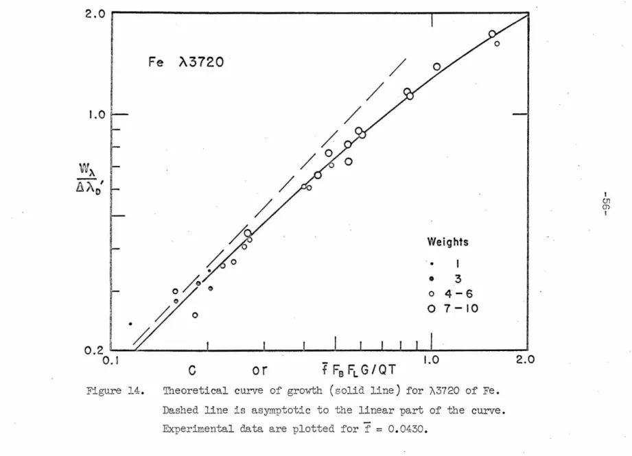
14 Curve of growth for Fe A3720 56

15 16

17 -18 19

20

21

22

23

Hyperfine and isotopic splitting

Curve of gro-wth for Cu A3247 Curve of growth for Cu A3274

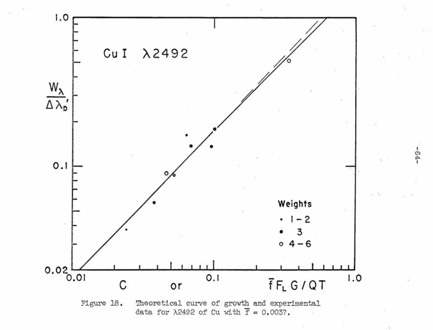
Curve of growth for Cu A2492

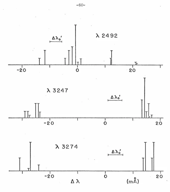
Hyperfine and isotopic splitting

Mean free path correction

Curve of growth for Cd A3261

Curve of growth for Cd A2288 Curve of growth for Au A2428

for copper

for cadmium

I INTRODUCTION

The oscillator strength, or f-value, of an atomic transition is a measure of the rate at ·which atoms absorb electromagnetic energy. If each atom which is capable of undergoing the transition is replaced by a "classical oscillator" consisting of an electron with an elastic restoring force such that i t has the same resonant frequency as the

original atomic transition, the absorption is easily calculated classically. The ratio of the energy actually absorbed by the atoms to that absorbed by classical oscillators is defined to be the f-value of the atomic transition.

In astrophysics, f-values are used to determine the abun -dances of elements in the solar atmosphere and in stellar atmospheres. Laboratory uses include measurements of the density and temperature of radiating atoms in plasmas and hot gases such as those produced by arcs and shock tubes.

Oscillator strengths raay be obtained theoretically if the electric dipole (or higher mul tipole for forbidden lines) matrix

-2

-The f-values reported here were measured with an atomic beam apparatus. The element under investigation i s placed in a cruc i-ble inside a vacuum chamber and heated to a temperature at which i t vaporizes. Atoms effuse out of a small orifice in the crucible forming an atomic beam the angular dimensions of which are defined by suitably placed knife edges. A light beam from a continuum source passes

r

through the atomic beam and into a spectro~aph where i t is analyzed to determine the total absorption of the spectral line being measured. At the same t ime the density of the atomic beam is moni tared by w

eigh-ing a part of the beam which deposits on a microbalance pan. From these measurements and the temperature of the crucible, the f-value can be determined. This method is limited to reasonably strong spectral lines of neutral atoms arising from low-lying energy levels which are populated at the temperature of the crucible.

The atomic beam method was first used by Wessel(2) and Kopfermann and Wessel(3) to measure f-values of Ba and Fe. Under the supervision of Professor Robert B. King at the California Institute of Technology, an atomic beam apparatus was constructed by M. H. Davis.(4)

Oscillator strengths of Cu, Fe, Mn, and Cr were measured with this apparatus and published by Bell, Davis, King, and Routly.(5,B,? ) In these measurements the absorption was measured with photographic plates and the atomic beam density with a sensitive quartz fiber spring

Major improvements in the apparatus ·were made by G. M. Lawrence and J. K. Link.(9,lO,ll) They used a photoelectric scanner mounted in the camera holder of the spectrograph instead of

photo-graphic plates to measure the amount of the absorption. In addition an automatically balancing electrobalance was used to continuously record the mass deposited by the atomic beam. Oscillator strengths of Cr, Co, Ni, Ga, Pd, Ag, In, Sn, Au, and Tl were measured with this apparatus.

The present work is a continuation of this project. A new, more sensitive, photoelectric scanner allows more accurate measurements of the weak absorption lines. The automatically r0 cording

-4-II THEORY

~he theory of the formation of absorption lines in an atomic beam was derived by Davis.(4) The following derivation leads to

similar results with the exception of the introduction of the parameter a'~

A. Atomic Beam Distribution

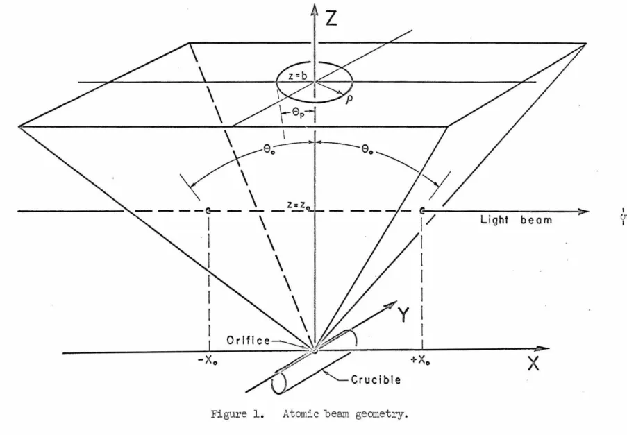
The geometry of the atomic beam and the coordinate system which vdll be used is shown in Figure 1. It is assumed that the distribution of atoms in the beam is given by the kinetic theory of gases for effusive flow through an orifice and that the size of the orifice is small enough that it can be treated as a point source. The validity of these assumptions is discussed elsevmere.

The number of a toms per second flm·dng through the orifice at an angle

e

from the normal, per unit solid angle, with speeds between v and v + dv, is given by Kennard(l2) as

7l (e) dv ==

v

3 3

-

t3

2v2

K

t3

v e cos

e

dv

where

../M/2RT

with M the atomic mass of the atoms, R the gas constant, and T the

(l)

(2)

absolute temperature of the crucible. The constant K is related to the density n

\

I

e

_o ~ _I

-Xo

-

_ _ _

,,_

e

~

I/

Light beam

I

I

I

I

I

I

I

+Xo

X

Figure 1. Atomic beam geometry.

I

CJl

-6

-K

=

At any point in the atomic beam the density of atoms with speeds

between v and v + dv i s

n (r,e )dv

v =

7Z (

e) v

2 vr

dv

₌

13

3 v2 _ 132v2

K ₂ e cos

e

dv r

where r is the distance from the orifice.

(3)

(4)

The light beam passes through the atomic beam at a height

z

0 above the orifice and is assumed to have negligible cross section. The quantity which will be needed is N (z )dv , the number of

v 0 x x

atoms per unit area with x-component of velocitJ between v and x

v + dv as seen l ooking along the light beam. Substituting

x x

r

=

z sec

e

and v

=

v csc

e

into equation (4) yields the density

0 x

distribution al ong the light path:

3 2 t3 v (z

,e

)dv K x n

2 e

v 0 x

x z

0

This equation must be integrated from

_

132v 2 csc 2

e

x

-x

0 to +x 0

3

e

dv ( 5)

cot

.

x

to give

N (z )av Consider the case v

>

O; the integral will run from

v _x 0 x _- x

0 t o +x only, since for negative x, no atoms have positive

0

x-velocities:

3

cot

e

dx ( 6)

With the substitutions dx z sec

e

ae

0 and then

2

integral can be done. The result is

=

K _R_ 2z

0 e

-(~

csc

e

)

2 v 2

0 x

(7)

Although this result was calculated for v

>

0 , the same result is x

obtained for v

<

0 , so equation (7) holds for all values of v •

x x

B.

Atomic Absorption

Since egua ti on ( 7 ) has the same form as the Maxwellian

velocity distribution for one component of velocity, the following

theory closely parallels the theory of the formation of absorption

t - d(l3)

lines by a mona omic gas. See, e.g., Unsol pp. 288 ff. or

Aller(l4)pp. 322ff.

The absorption coefficient per atom as a function of

frequency vis given by the Weisskopf-Wigner formula:

Cf,

v = 2 ne

me f

(v - v)

₀ 2 +

(r/4rr)

2 (8)

where f is the oscillator strength of the absorption line centered

at v , e and mare the charge and mass of an electron, c the velocity

0

of light, and

r

is the radiation damping constant of the line. If

the atom is moving, the center of the line is Doppler shifted from

v + v

v /c

0 0 x

Cf, v

2 ne

me

so equation (8) becomes

f

v

/c -

v)2

x

2

-8-The optical depth ~ is obtained by multiplying equation

v

( 9) by N ( z )

v 0 x

and integrating over v :

x

+oo 2

KL~f

2z me

0

J

2 2

-(f3 csc

e

)

v

0 x

e

(v + v v /c - v)2 + (r/4rr)2

-oo 0 0 x

This integral is conventional ly written as

CH(a ',u)

where the following substitutions have been made:

c

==

H(a',u)

a'

u

y

2

KL

rre f ..£._

2z me v

0 0

+oo 2

1 a' e-y

rr

J

2

a' + (u - y) 2 - co

r/4rr

==

b.vD I

v - v 0 b.v '

D

v

x c

damping ratio dy

dv x

f:,V I

D

VO

sin

e

f3c o

v

~

.J

2RT/M sin

e

c 0

Doppler width

(10)

(11)

(12)

(13)

(14)

(15)

(16)

(17)

The Doppler vddth and damping ratio are primed to distinguish them

from the corresponding quantities with sin

e

removed which arise

in the theory of absorption by a gas.

The i ntensity I of the transmitted light is given by

v

--r -C H(a' ,u)

:t _v = I ₀ e v == _Io e (l8)

"Where I

0 is the intensity of the incident light .

. C. The Curve of Growth

Since the width of the line profile given by equation (18) is much smal ler than the resolution of the spectrograph "Which is used, a measure of the total amount of light absorbed is needed. This quantity i s the "equivalent width" defined as

w

v

J

line

Using equation (18) this becomes

where the limits of integration have been extended to + oo •

(19)

(20)

At this point it is convenient to express the formulas in terms of wavelength A

=

c/v instead of frequency v because the experimental.measurements are made in terms of

A

·

Since the absorp -tion line·s are very narrow, no error i s made in setting

(v -

v,;>

= Ac2 (A - Ao) 0

-10- '

This equation also applies if (v - v

0 ) is replaced by 6vn' or

Wv with (A - A

0 ) replaced by the respective quantity in wavelength

units. With these changes, equation (20) becomes

WA

j

{1

e-CH(a',u)} du ₍₂₂₎

!SJ\ I

=

D _{- oo}

"Where

A

~'

₌

_c 0 ..) 2RT/M sin

e

( 23)

0

2

c

₌

K __§_ _{2z me} 1(e f A ( 24)

0

0

A 2

r

a'

₌

0 ( 25)

41(C MD I

In addition equations (11), (15), (16), (18), and (19) are valid if

every v, 6vD', W v' etc. is replaced by A, 19\D', Wt/ etc.

For the lines considered in this work the parameter a' can

be expressed in terms of the f-value. The damping constant can be

written as (see Aller(l4) pp. 172-176)

r

where for any state i,

1

,..i

I

j

A ..

1J

( 26)

and

A ..

l.J

=

2 2

8rc e 2

me Aij

f ..

Jl. (28)

The subscripts u and P, refer to the upper and lower energy levels

for the transition under consideration, ~- is the lifetime of the

1

state i, A . . is the Einstein coefficient for spontaneous transitions

l.J

from state i to j, g. is the statistical weight of level i and is

l.

equal to (2J + 1), and f .. is the absorption oscillator strength Jl.

for the transition j -7i which has been and will henceforth be

referred to simply as f. The summation in equation (27) extends

over all levels j that are below level i. For the transitions under

consideration, level £ is either the ground state or in any case has

~p,

>>

~u so that r;, can be neglected. Also, the only term in the

summation that is important is Au£' i.e. the A-value for the line

being investigated. With these restrictions, equations (26), (27),

and (28) can be combined and substituted into equation (25) to give

a '

For special case a'

(13) simplifies to

2

2rce 2

me !SA '

D

(29)

o

,

it can be shown that equation

H(O,u)

2 -u

e (30)

-12-=

7

{

1 - exp (C e-u 2

) } du ( 31)

-oo

If the exponential is expanded in a Taylor's series the integral can

be evaluated term by term giving

{

c2

== -!rt

c

-

2 ! J' 2 +

c3

3! J'3

+

...

}

(32)

Unsold(l3) p • . 290 also gives an asymptotic expansion which is useful for large C.

The relation between WA/D.AD' and C given by equations ( 22) or ( 32) is knmm as the curve of growth. It shows how the

strength of the absorption line varies with the number of absorbing

a toms. Moise ( 15 ) A pp • C gives tab le s of the curve of growth for various values of the damping ratio. Figure 2, plotted from these

tables, shows the form of the curve of growth for various values of

a'. The portion of the curve for C

<

1/2 is known as the linear

part. For intermediate values of C the curve flattens out and

becomes dependent on a'. For large C the curve approaches the

asymptote WA/ 191.D ' = 2

.J

._frt a , C . •

Experimentally, values of C are obtained from the curve of

growth and the measured values of WA. As the slope of the curve

.

~

0

~

G-l

0

{/)

<V

~

C>

..--l

0

ell

C>

·

rl

.µ

<V

H

0

<V

0

~

.

C\J

<V

5

00

·rl

~

-l4-the fainter -l4-the line, -l4-the less accurately i t can be measured. For these reasons most of the experimental data are taken on the upper end of the linear part, near the "knee" of the curve.

For most of the lines considered here the value of a 1 _is

less than 0.01, and in the region of interest the curves for

0

<

a 1

<

_{0.01 are virtually coincident so the curve of growth may}

b~ approximated by equation (32). However, for A2288 of Cd, data can only be obtained above the linear part. This line also has a large value of a 1 _{so the curve of growth must be calculated using}

equation (22) (modified as described in Section II-F because of isotopic and hyperfine structure).

D. The Deposit Rate

The value of K is determined by weighing the atoms which go through a circular aperture of radius p at a height z = b above the orifice as shovm in Figure 1. The rate 7Z at which atoms go

p

through this aperture is obtained by integrating equation (1) over velocity and the solid angle

n

of the aperture measured from the

p

orifice:

co

np

J

dv

J

an

n

_v (e)

0 _DP

e

co

[32 2

/cos

K f33

J

_v3 e - v dv

e

2rc sin

e

de

0 0

re K . 2

e

=

_2"13

sin

2

( b2 p 2 )

+ p

(33)

When these atoms deposit on the microbalance pan the rate at which

mass is added is

G == M _N 0

n

_p

where N is Avogadro's number.

0

== :rr K M

2 ~ N

0

(

2 p )

2 2

b + p

Equations (2), (24), and (34) can now be combined and

solved for the f-value:

where

Q

f ==

2Rrnc

N e2

0

QT C G

z 0

Ao (

2

p )

2 2 b + p

(34)

(35)

( 36)

and C is obtained from the measured value of WA and the appropriate

curve of growth.

E. The Boltzmann Factor

For most of the elements studied with the atomic beam

apparatus the excited states are sufficiently separated from the

ground state so that, at the temperatures necessary to produce an

atomic beam, essentially all the atoms are in the ground state and

-16

-however, have several low-lying states which are appreciably populated at these temperatures, and in this case the deposit rate must be mul -tiplied by the Boltzmann factor

-Ep,/kT gp, e

FB

I

gi e -E./kT i ( 37) i

where E. is the energy of the ith level and k the Boltzmann constant. J_

In applying this factor i t is assumed that the relative populations of the atoms in the atomic beam are the same as in the crucible. While the radiative lifetimes of these levels are long enough that they do not return to the ground state in the time i t takes them to travel

from the crucible to z

=

z

0 , Lawrence( 9

) finds some evidence that

levels with E.

>

kT may be depopulated, perhaps by collisions in J_ ""'

the atomic beam.

F. Hyperfine Structure and Isotope Shifts

Most of the lines studied have hyperfine and isotopic structure which is, at best, only partially resolved by the spectra -graph. The theory which is derived for a single line in Sections B

and C must be modified to take this into .account. If the line

consists of n components, of which the ith component has fractional strength

I.

and is centered at

A.,

then equation

(22)

generalizes

J_ J_

"Where

-

c

= - e

- co

=

/\.

-

/\

J.. 0

M I

D

and

n

z

i=l

I.

J.. H(a',u-u.1 )

} du

= 1

If the hyperfine and/or isotopic splittings are smal l ( 38)

compared to the Doppler ·width of the line, i .e. all u.

<<

1 , then

J.. .

they wil l have little effect and equation (22) can be used. On the

other hand, if the splittings are al l large, (u. - u.)

>>

1 for

J.. J

all pairs i

f

j , then each individual component does not overlap any other and each will follow its own curve of growth. The total

curve of growth for the unresolved group is then

==

Thus, for any C,

l

n +!.co { 1 - e -C I 1 . H( ' a ,u ) } du i=l - co

w

/M I = /\ D

n

I: i=l

(39)

obtained from the single component curve of growth, equation ( 22 ),

for C. = I. C . It is clear that the same procedure can be followed

J.. J..

- lB

-compared to L'-t-D', and each group is separated f'rom the others by distances -which are large compared with MD'. Qualitatively it can be said that if' the total spread within each group is less than

1/2 MD' and the centers of' gravity of' neighboring groups are sep-arated by more than 3

Mu',

then the curve of' gro-vrth given by equation (39) can be relied on at least half' way up the "knee."

If' these condftions are not met, then either measurements

must be made only on the linear part ("Which is fortunately extended

by the splittings ) or else . the exact curve given by equation ( 38) must be calculated numerically.

G. Impulse Forces

When the shutter under the microbalance pan is opened,

the pan experiences an upward f'orce due to the momentum of' the atoms

in the atomic beam. Assuming all of the atoms stick to the pan, this force ~is given by the rate of momentum transfer in the

z-direction of the atoms impinging on the pan:

00

';}- ₌

J

_dv

J

an

_Ii-

_{v cos}

_e

_7z

₍

_e

₎

N v

0

0

n

p

e

00

-f32v2

f

M _{K (33}

J

4

dv 2

N v e

_J

cos

e

2n sin

e

de

0

0 0

3/2 _{M K}

{1-

3

eP}

1l

=

- -

cos

4 _N

1(3/2 M K

4 N f32

0 b

2 2

+ p

)3/2}

(40)

A more convenient quantity to measure is the ratio of the impulse force to the deposit rate. TI1is quantity, known as the

recovery time tR because it is the time required for the micro

-balance output to return to its value previous to opening the shutter, is given by

=

:1

gG

where g is the acceleration of gravity. TI1ese recovery times range

between 0.5 and 2.0 minutes.

It is convenient to expand equation

(

41

)

in a power series

in (p/b )2 :

(42)

In practice (p/b)

;S

0.11 so less than O. 3°/o error is made in using

only the first term of the series.

H. Impulse Force Anomalies and Deposit Rate Corrections

TI1ere are several reasons why the experimentally measured

-20

-mechanism producing the discrepancy is knownJ an appropriate correction can be applied to the deposit rate. The possible

mechanisms are: (1) Non-constant atomic beam fluxJ (2) The presence of molecules of the element being studied in the atomic beamJ (3) Non-unity sticking coefficient of the atoms on the panJ and (4)

Adsorption of residual gas by the metal deposited on the balance pan. These mechanisms are considered in detail in the Appendix. The

results are that mechanism

(1)

can be recognized and the data dis-carded) and that (2) to (4) lead to correction factors of a similar nature Which can be applied to the observed deposit rate.

Let the observed deposit rate be (l +a) times the deposit rate Which would have been obtained if all the desired atoms and no others stick to the pan. Then

l

-A+ ( t obs /t th)

R R

a =

where t obs

R is the observed recovery time and

t th

R is the

(43)

theoretical value given by equation (42). The constant A is given by

l/,fn for n-atomic molecules (44)

-

_{in the atomic beam}

A =

5.JTJT

for non-unity sticking ( 45)

3 p coefficient

vfuere Tp is the temperature of the pan and MA is the molecular weig_ht of the adsorbed gas.

The observed deposit rate may be multiplied by

1 _ <-1-) < 1 _ t obs

It

th )

1 +A R R ( 47)

to give the corrected deposi t rate. As shown in the Appendix) the value of 1/(1 +A) is approximately 0.5 to 0.8 but can rise to

3.414 if diatomic molecules are present in the beam. Even in the ka

absence of any knowledge of the mec;;i;;.nism, an average value of 0.6 to 0.7 should give corrections vfuich are good to 10%,and if the corrections are no larger than 10% then the corrected deposi t rates should be good to 1%. This assumes that the anomaly i s not due to molecules, in vfuich case the correction would be much too small.

Even if molecules are suspected) the use of the corresponding value of 1/(1 + A) is very risky because small errors in t obs

R due to

other mechanisms or instrumental errors would be greatly magnified.

I. Summary

In order to measure an f-value, the following quantities must be measured: equivalent width WA (nJ?), deposit rate

G (µg/min)) crucible temperature T (°K), and v~rious geometrical factors z ' b, p (inches)) and sine.

0 In addition the wavelength

A

(

R

)

of the line) any hyperfine and/or isotopic structure, and 0

-22-The numerical factors in the fol lowing equations are

appropriate for the units given in parentheses. Using equation (23) the Doppler width MD' (mR) i s calculated:

M I

D

Ao

.J

2RT/M sin

e

c 0 4. 3021 x

10-4

"o sin

e

0

.fT7M

. (

48)

A value for f is estimated and the value of a ' is calculated from

equation ( 29):

2 A"\ I

m c Ll/\D

0.17705 ( 49)

a '

Then C is obtained from the appropriate curve of growth, equation (22), (32), (38), or (39). Finally, the f-value i s calculated from

f

where Q is given by

Q

2 2 {? 2 ) b + p

Either FB or FG or both may be unity.

(50)

z 2

498.10 " : ( b2 : p2 ). (51)

In principle i t would be necespary to put the resulting f-value back into a ', and then iterate to obtain a consi stent result. However, in practice, this is not necessary since the region of the knee of the curve of growth on whi ch the data usually falls is qui te

III APPARATUS

A. Vacuum System

The vacuum chamber and atomic beam furnace have been described by Davis. (4) The furnace is enclosed in an 8 1/2 inch diameter brass cylinder 10 inches high with quartz windows sealed to

two side arms which let the light beam through. A 1/2 inch thick brass

bas.e plate contains electrical and -water cooling feedthroughs f'or

the furnace. The microbalance is mounted on a 1/2 inch thick aluminum

alloy plate which rests on top of the brass cylinder and is covered with a glass bell jar. There are approximately thirty demountable

seal s using viton 0-rings.

The vacuum is produced and maintained by a Kinney 4 inch

diffusion pump with a 5 cu ft/min Kinney forepump. Dow Corning DC-705

silicone pump oil is used in the diffusion pµ.mp. There is a liquid

nitrogen cold tra.p in a -water cooled baffle above the diffusion pump.

The ultimate pressure which can be attained is slightly below 10- 7 torr

.as measured ·with a Veeco RG 75K ionization guage. However, the pres

-are

sure is usually at least ten times higher while data ~ being taken

because of outgassing caused by the hot furnace.

B. Atomic Beam Furnace

The element to be vaporized is placed in a cylindrical

crucible of graphite or zirconia and heated in a furnace tube of

-24

-crucible forms the source of the atomic beam. The furnace tubes must have a larger hole in them to provide clearance for the beam. Details

of the crucibles and furnace tubes are given by J. K. Link.(lO)

The ends of the furnace tube are clamped in water-cooled

copper blocks and the furnace is heated by up to 300 amperes of alte

r-nating current. Power for the furnace is provided from a ll5 v line

by a 3 kv Sola constant-voltage transformer, and the furnace power is

controlled by a 40 amp Variac. The constant-voltage transformer makes the furnace power regulator, -which was formerly used by Davis ( 4) and

Bell,(5) unnecessary. Temperatures in the crucible of over 2000° C

can be produced if the furnace tube is surrounded by a radiation shield. The furnace is surrounded by a water jacket with a slot in

i t which defines the solid angle of the atomic beam. A water-cooled

plate with the circular aperture, -which determines the portion of the

atomic beam -which goes to the microbalance pan, is mounted 7 inches

above the furnace. Between this plate and the pan there is a shutter which is operated manual ly from outside the vacuum chamber.

A window is provided in the vacuum chamber for sighting into

the orifice of the crucible with an optical pyrometer to measure the

temperature. Because the atomic beam deposits would otherwi se darken it, a disk of glass is installed under the window which can be rotated

from outside the vacuum chamber to provide a clean surface for each temperature measurement. Besides the ·window and disk, there is a

right angle prism outside the chamber to obtain a more convenient

the pyrometer so a correction curve was obtained by measuring the

temperature of a tungsten ribbon lamp with and without the windows and

prism. The

c~rrections

range from 15° C at 800° C to 69° C at 2100° C.

Cadmium vaporizes at temperatures which are much too low to

measure with an optical pyrometer, so a special graphite curcible was

constructed with a platinum to platinum - 10% rhodium thermocouple in

it. The thermocouple was contained in an alundum thermocouple tube

with the end cemented over with Saueriesen #7 cement. This tube pro

-truded through one end of the crucible with the thermocouple junction

under the orifice and was cemented in place with Sauereisen.

The thermocouple was compared with the optical pyrometer at

0 0 0

temperatures between 800 C and 1500 C and found to read 12 C to

40° C low with the largest difference at low temperatures. A rough

theory considering heat conduction along the thermocouple tube and

radiation from the walls of the crucible to i t accounted for these

differences i f the heat conductivity of the alundum tube was properly

chosen. At low temperatures the difference should rise linearly with

the difference from room temperature; the difference reaches a maximum

and then falls at high temperatures because of the increased transfer

of heat to the tube by radiation from the crucible.

In practice, the freezing temperature of cadmium (320.9° C)

-was observed by the step on a cooling curve and the corrections ·were

assumed to be linear with the difference between room temperature and

the crucible temperature. While the correction varied between l l

°

C

-26-during any one run. C. Microbalance

The microbalance was originally built by G. M. Lawrence ( 9)

with the electronics designed and built by the present author. Since the work of Lawrence, Link, and King, (ll) the electronics have been

.

rebuilt to provide about a factor of ten reduction in noise. In addition, most parts of· the microbalance itself have been replaced because of breakage.

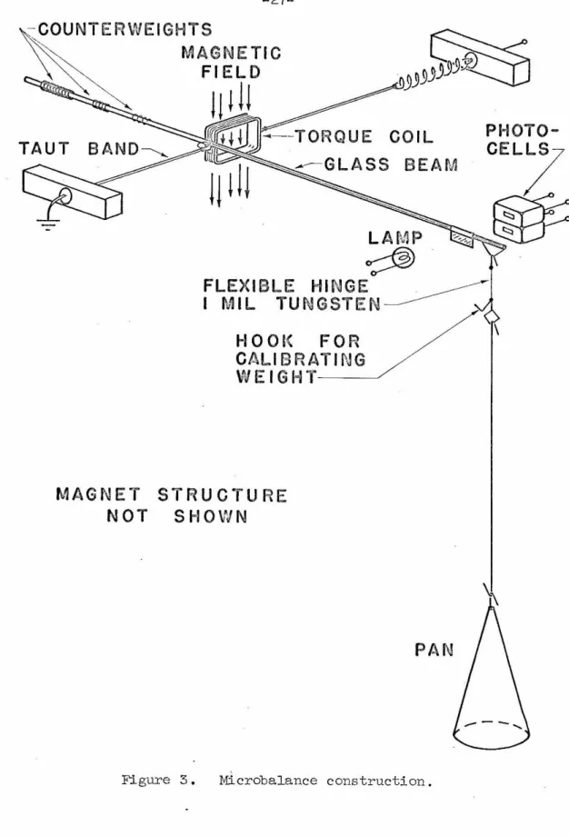
Figure 3 shows the structure of the microbalance. It uses

the magnet structure and torque coil of a small 0-500 µA panel meter.

The pivots have been replaced with a taut band susp·ension system in

"Which the springs, which originally provided the restoring torque for

the meter, have been stretched out and soldered to the tips of the

original pivots to fonn the taut bands. A small spring provides

tension.

The pointer has been replaced with a beam made from a drawn

out glass tube about 0.030 inch in diameter and 5 3/4 inches long,

which is cemented to the coil at one of the pivots with polystyrene cement. The pan i s suspended from one end of the beam 3 1/4 inches

from the torque coil. Three counterweights made of different sizes

of copper wire can be slid along the other end to adjust the static

balance.

Pans weighing about 30 mg are made from 0.25 mil thick

LAMP

o;:@

FLEXIBLE HINGE

.

---I

MIL TUNGST

EN---

- ,

l-IOOt<

FOR

CALIBRATING

WEIGHT-~

MAGNET

STRUCTURE

NOT

SHOWN

PAN

Figure 3. Microbalance construction.

-

28-fo:rmed into a cone with a 1/16 inch wide folded seam. Approximately

l/16 inch of the open end is folded inward providing a more rigid

structure, and a small hook of 5 mil diameter aluminum wire is attached

to the apex. The pans are made conical to increase the fraction of the

incident atoms which stickj any atom which does not stick on the first

encounter has a good chance of hitting the pan again.

A 5 mil nichrome wire passes through the microbalance beam

from the torque coil to the end where i t is formed into a stirrup.

This grounds the pan, removing the possibility that i t might become

electrically charged. Such a charge, if i t raised the pan to a paten

-tial of 100 volts, would resul t in spurious forces of approximately

12 µg as the shutter was operated.

J . K. Link(lO.) .found that placing a l ight bulb near the pan

partial ly prevented the adsorption of residual gases by the fresh

deposi t. In the present experiment this function is provided by

several turns of nichrome wire which surround the pan and may be

heated red hot. The use of the pan heater is described in Sections

IV-B

,

C

.

A permanent magnet is placed near the pan to damp out

pendulum oscil lations by means of induced eddy currents. Tne magnet

could not be used for atomic beams of iron so the flexible "hinge"

shmm in Figure 3 1-;as replaced by a rigid support wire and damping·

vra.s supplied by sliding friction at the stirrup. This method of

suspension leads to greater noise in the output si gnal due to changes

The microbalance is balanced by adjusting the current

through the torque coil until i t is at rest at a given position so that changes in the current are accurately proporti onal to changes in the mass of the pan despi te any variation of the strength of the mag -netic field -with angle. A feedback system keeps the microbalance

continuously balanced. The position of the beam is sensed by two RCA 6694-A cadmium sulfide photocell s illuminated by a number 222

prefocused flashlight bulb. A flag on the beam covers one photocell

and uncovers the other as the beam moves. The output of this detector

is amplified by a two-stage complementary transistor amplifier as shown

in Figure 4, and the output is fed back to the tor;ue coil through

resistor R and capacitor C

0 0 The capacitor provides feedback

propor-tional to the velocity of the beam and is chosen to produce nearly critical damping. The feedback gain is greater than 1000 and produces

a restoring t orque much greater than that of the taut band suspension

system. In fact the mi crobalance itself is mechanically unstable

because the beam is cemented above the taut bands, and thus i t cannot be balanced -with out the automatic ·feedback system.

In addition to the current produced by the amplifier, current in the torque coil can be varied manually through resistors R

1 and R2•

In use the manual balance controls are adjusted so that the amplifier output is near zero. The amplifier can supply a current equivalent

to + 2.2 mg and the manual controls + 5.5 mg.

The output of the amplifier is filtered by capacitors

c

1 and

c

+9v +12 v

Figure 4.

-30-20K

TOTAL MASS

t 5m~

t250)lA

+12v +9v

Microbalance circui t .

--- ---·-· - - - ---· --- ---· ---

--5 "''

chart recorder. The following ranges are provided: 5, 10, 20, 50, 100, 200, 500, and 1000 µg full scale.

The power supply for the microbalance electronics is well

stabilized by Zener diodes. The power to the manual balance controls

must ce especially well regulated as can be seen from the follmting

consideration. When these controls are providing a current to the

coil equivalent to 5 mg, a shift in that current of only 0.01% will cause a shift in the output of 0.5 µg.

The microbalance is calibrated by hanging a 1 mg class M

weight from a hook on the pan suspension and adjusting the calibration

control R

3 until the weight produces full scale deflection of.the recorder on the 1000 µg scale. A manipulator allows this to be done while the vacuum system is pumped down.

Fluctuations in the microbalance output amount to 0.04 µg

peak-to-peak and drift is less than 0.005 µg/min when the equipment is thoroughly warmed up. The response to a sudden change in mass shows a rise time of 0.0035 to 0.005 minutes (0.2 to 0.3 sec.) depend-ing on the amplitude on the chart recorder. This is small enough so that it does not affect the measurement of recovery times.

Tracings of two microbalance recordings are shown in

4

mass

3

(JJg)

2

40

moss

30

(.ug)

20

I 0 pen

4

-32-Close

Drift• 0.004 pg/min

~~

·

"

'

O. 016 µg/min

Lscan

14

G = 0.191µg/min

8

2

13 G=0.222·µg/rnin

12 G"' 0.216 µg/rnin

12 time 16 20(min) 24

28

tRs0.62

mini

3 time 4

__

,.,.__

__ _

/

/ /

shutter

G = 7.15 µg/min

5 (min) 6 7

32

8

D. Optical System

Figure 6 is a diagram of the optical system. Light from the

horizontally mounted capillary tube of the lamp is imaged in the atomic

beam by lens #1 (approximately 15 cm focal length) and reimaged on the

spectrograph slit by lens #2 (25 cm). These lenses are made of quartz

and are not achromatic so the optical system must be refocused for

each wavelength. This is accomplished by adjusting the positions of

the lamp and lens #2. The st op is a 1/4 inch diameter aperture placed

around the virtual image of the spectrograph grating to eliminate

extraneous light. The light modulator varies the amount of light

reaching the spectrograph in such a way as to remove fluctuations in

the intensity of the lamp.

In developing the theory) it was assumed that the transverse

dimensions of the light beam are negligible as it passes through the

atomic beam. This) of course) refers only to that part of the beam

which is subtended by the grating and is diffracted to the phototube.

The thickness of thi s beam varies from 0.08 mm directly over the ori

-fice to 1.0 mm as i t enters and leaves the atomic beam. The hori zontal

width is 7.2 mm. Compared with the hei ght above the orifice (z ) of 0

2.5 cm, these dimensions are small enough that less than 1% error i s

made by the assumption that the transverse dimensions of the light

beam are negligible.

The light source is a PEK Labs type A high pressure mercury

arc lamp operated at 500 to 1500 v de from a motor-generator set. It

length of 1 mm bore quartz capillary tube, which is surrounded by a quartz water jacket. The lamp is cooled with tap ·water, which slowly deposits salts on the capillary tube and water jacket resulting in a gradual decrease in the intensity, especially at very short

wave-lengths. These deposits may be removed with dilute hydrochloric acid. Figure 7 shows the spectrwn which is produced by the lamp in this optical system. It is similar to the spectrum obtained by Stahl(l5) and consists of pressure-broadened emission lines with strong continuum radiation between them. The drop-off in intensity

at the extremes of the spectrum is due partly to the blaze of the spectrograph grating. It is of interest that in regions near emission

lines or below 2500

R

the intensity decreases with increasing power

to the lamp. All data reported here were obtained in wavelength regions far removed from any of the emission lines.

The filter shovm in Figure 6 is used to limi t the light reaching the spectrograph to that in the desired order. For wave-lengths between 3500

R

and 3900 ~ a Corning glass filter no. 7-59 "Blue Purple ffitra" is used. Between 2800

J?

and 3500

1\

the filter is no. 7-54 "Red Purple Corex A."· Below 2800

J?

a liquid filter is used,

"Which consists of a solution of 180 g NiS0

4·6H20 plus 80 g CoS04·7H20 per liter of water contained in a quartz cell with a thickness of 3. 5 cm. This filter is a compromise between those recommended by

. (17) (18)

100 10 1.0 PHOTOTUBE

CURR

ENT

0.1 I I I I -3

6-.

,, " " " ,, :· ,. ,.

,,

I

.

.

I

.

_{' ,}

.

.... /

.

\

,

·•

·

...

,,

·

..

PEK Labs Type A Lamp

1500 volts

-·--·-

1000 volts

---·

-

---

--··--

500 volts

10-! -~-.1, ___ _.. ____ ..., ___ _...._

2000 3000

WAVE LENGTH

4000

X

Figure 7. Lamp spectrum.

Cl

(A)

'•

\ \ \

•.

'

.

\

_.

I

'.

_{' I}

f

"

....

/

The light transmitted through the atomic beam is analyzed

by a 2l foot Rowland spectrograph. The Bausch and Lomb grating has

a radius of curvature of 6.65 meters and a ruled area l 3.8 cm long

with 600 rulings per mm .. It is used in second order where the disper

-sion is l.253

R/mm.

The entrance slit was set at l5 to 40 microns

with an exit slit of 2l microns. Figure l 3b gives an indication of

the resolution which can be obtained. The hyperfine components of

the copper line A3247, which are about 40

mR

apart (see Section IV B),

are partially resolved. Theoretically the resolution of the grating

at this wavelength is 20

rnA',

but this is degraded to more than 35

rnA'

because of the finite widths of the slits.

The amount of scattered light in the spectrograph has been

estimated by inserting filters in the light path which cut out the

wavelength for which the spectrograph is focused and pass large bands

of the spectrum at other wavelengths. At wavelengths above 2500

R

these measurements indicate that the amount of scattered l ight is

negligible. Ho-wever, below 2500

R;

where the light intensity is small compared to the intensity at longer yre,velengths, significant amounts

of scattered light are present and must be taken into account. As

described in Section IV-C, 12.6% of the photocurrent at 2288

R

was

found to be due to scattered light.

At the camera holder of the spectrograph there is a carriage

containing the exit slit and photomultiplier tube detector which are

scanned along the focal curve to record the spectrum. In addition,

-38-mirrors whJ.ch supplies a signal to the light regulator system. This carriage replaced a similar one used by Lawrence and Link, ( 9 ,lO,ll)

in which a reference signal was obtained through a light chopping

arrangement.

The exit slit was constructed from razor blades in the manner

described by Lai;vrence, (9) p. 34. In keeping with advances in the state

of the art, Wilkinson Sword stainless steel blades were used instead of

the Gillette Super Blue Blades previously used. The width of the slit

varies from 20 t o 23 microns over a length of 2 cm with an effective

average being 21 microns.

The light passing through the exit slit i s detected oy an

EMI/US type 952613 photomultiplier tube which has a quartz end window.

Its response extends from below 2000

R

to above 6000

R.

The dark

current is less than one nanoampere, which is negligible compared to

the signal· current which is usually between one and three microamperes. Power for the photomultiplier tube is obtained from a

John Fluke model 402M high voltage power supply which is regulated to

0.01%. Typically, the voltage was set at 1200 to 1300 volts except

for wavelengths below 2500

R

where voltages up to 1600 vol ts were used

because Of the smal l amount of light available.

The carriage is driven up and down the focal curve of the

spectrograph by a Starret no. T465P micrometer head. Power is supplied by an Apcor model 2201-60 multiratio gearmotor coupled to a thirty-to

-one worm reduction gear. Except for the multispeed gearmotor, this

LIGHT FROM

GRATING

Figure 8.

BELLOWS COUPLING

MICROMETER

HEAD

Carriage.

SCANNER

· MOTOR

I

(fl <..O

-40

-scanning speeds which are available are: 1) 2.5) 5, 10, 25, and 50

mils per minute. Most of the data was taken with a scanning speed of

2.5 mil/min although 5 and 10 mil/min were also used. The faster

speeds are useful for finding lines.

Since the widths of the absorption lines are only about

2 to 3 mils at the focal curve of the spectrograph) the motion of the

carriage must be very precise. Al though the carriage is driven by a

synchronous motor so that i ts average speed is constant) there

occasionally appears to be short-term variations in the scanning

velocity. This.is indicated by comparing average f-values obtained

while scanning in the two directions; if the difference is .greater

than the scatter in the individual values) velocity variations are

suspected. Attempts to measure the instantaneous velocity of the

carriage have been only partly successful due to its extremely small

value. However, at one time an increase in velocity of approximately

13% for one-half minute was observed along with several smaller

increases and decreases. These variations were observed while

scanning in one direction but not the other. Most of the time, the

scanning velocity seemed to be constant to within 2% when averaged

over 10 seconds. Disturbances such as these are minimized by care

-fully polishing the track in which the carriage slides with #600

emery paper and lubricating it with "Lubriplate."

E. Light Regulator

measured at different times as the carriage is driven across the

spectrum, i t is important that the intensity of the continuum be

constant with time. Unfortunately the light output of the lamp

fluctuates. These fluctuations consist of continual variations of

about 1%, sudden jumps in the intensity of about 10%, vihich

occa-sionally occur as often as every minute or so (or occasionally not at all), and a long term decrease of up to 10% per hour due mostly to

the deposition of cooling water contaminants on the lamp and water

jacket. The_ purpose of the light regulator is to remove these

fluctuations.

The light regulator operates by forcing the output of the

reference photomultiplier tube to remain constant. It does thi s by

varying the fraction of the lamp 1 _{s output which reaches the spectro}

-graph through the action of the light modulator and also by varying the power to the lamp.

As shown in Figure 8, the 1P28 reference photomultiplier tube is mounted on the carriage and, by means of mirrors, looks at

two bands of the spectrum which straddle the portion seen by the

detector photomultiplier tube. Experience has shown that fl uctua-tions in the lamp output at different wavelengths are poorly

correlated if the wavelengths are not close together. Tnerefore, the

two bands seen by the reference tube are made .small and close

together. },igure 9 shows the response of the reference system in

relation to the detector ·wavelength as measured by scanning a

- 42

-DETECTOR PH OTOTUB E

-4 -2

"A - "Ao

0 2

<Al

SIGNAL

4

Figure 9. Relative response of reference photomultiplier tube.

LIGHT

FROM

LAMP

KNIFE

VOICE COIL

LEADS

Figure 10. Light Modulator.

SUSPENSION

VOICE COIL

The entire reference signal comes from wavelengths within + 2 l/2

R

of the -wavelength seen by the detector tube.

The light modulator -was constructed from a small loud

-speaker as shmm in Figure lO. The cone and excess sheet metal were remoyed and a bakelite knife edge -was cemented to the voice coil.

Its resonant frequency is 100 cycles per second with a damping ratio of 0.45. It is placed in the light beam between the stop and the filter as shovm in Figure 6 and .is positioned so that i t blocks out approximately 25% of the light to the spectrograph. As signals are applied to it, the voice coil moves up or dovm blocking out more or

less light.

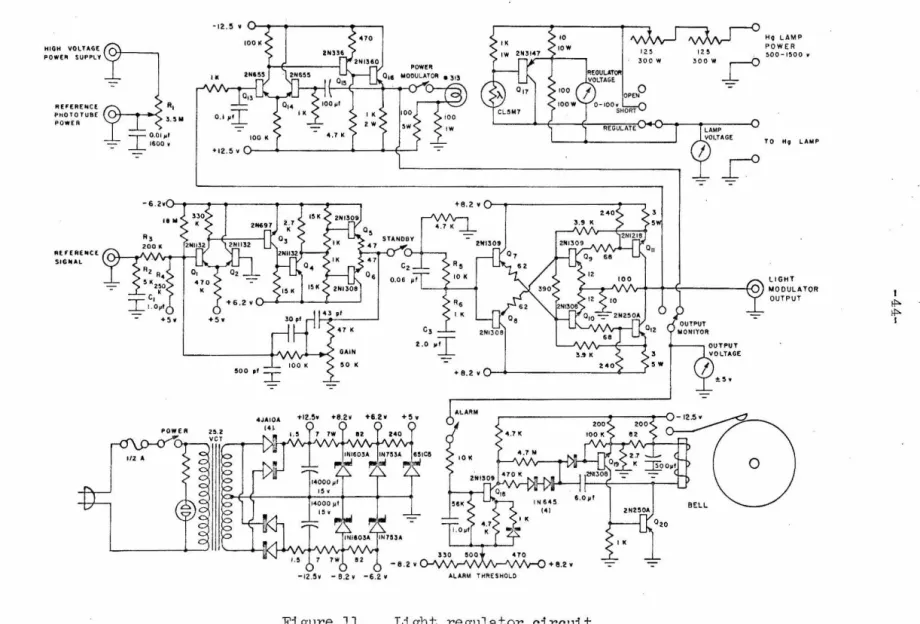
The circuit diagram of the light regulator is shovm in

Figure 11. Voltage for the reference photomultiplier tube i s obtained . from the same power supply that powers the detector tube but can be

varied from 40 to 100% of that voltage by!\· This control s the gain of the phototube, which is always operated with a photocurrent of 20 µA regardless of the light level.

The current from the reference tube is filtered by R

2, R3,

and

c

1 to reduce the high frequency response so that the amplifiers are not overloaded by noise due to statistical variations in the rate at which photons reach the phototube. A constant current of 20 µA

is subtracted from the photocurrent through R

4 and the difference is

amplified by a preamplifier consisting of transistors ~ through ~ and their associated components. The gain of this preamplifier can

HIGH VOlTAGE

POWE" SUPPl.'t

'HHRENCE

PHOTOTU8£ POW[A

RE HAElllCE

SIClllAL

-::- -=-"• :S.$ ..

c,

i

.

o,,I

-=-

_-

_.

-•e.2vO---i~~~~~~~~~_.~~

-t-IZ.Sw +8.2 v t-1.2 w + S w

±0•

-=-LIGHT

MODULATOR OUTPUT

~8

Nv--+-/)~~K ~OJt

_{2M308 - '} 0

BELL

-12.sw -e.2 w -6.2 w AL.AAM THftE5HOU)

Figure 11. Light regulator circuit.

I

capacitors associated with the gain control are necessary to elim i-nate high frequency instabilities.

The output of the preamplifier i s applied to a compensation

network consisting of R

5,

c

2,R6, and

c

3. This is a "lead-lag" net-work •mich adjusts the frequency and phase response of the overal l feedback loop so that i t is stable. The component values were chosen

by the use of root-locus plots.

The light modulator is driven by a complementary ampli fier with transistors ~ through ~

₂

• This amplifier has a high input

impedance so that i t does not load the compensation network and has

an output voltage swing of + 5 volts into the 6 ohm impedance of the

l ight modulat or.

After operating the light regulator with these components,

i t was noticed that, although the total gain i s more than 60 db, changes in the light intensity due to changes in the lamp power were

not completely removed. This suggested that additional improvement

could be obtained by modulating the power to the lamp.

The lamp power is modulated by transistor ~

₇

, .mich is

controlled by a cadmium sulfide photocell illuminated by a small lamp. In this manner signals are transmitted to ~

₇

despite the 500 to 1500 volt potential between it and ground. In considerati on of the maximum voltage and power ratings of Q

17, the range over which

i t can vary the mercury lamp vol tage is limited to about 100 volts.

In practice, this has usual ly been sufficient although there have

-46-The #313 lamp is driven by ~

₃

through ~

₆

which amplify the voltage applied to the light modulator. Thus) the lamp power modulator circuit forces the light intensity to be such that no action is needed by the light modulator.

It would seem much simpler to eliminate the light modulator and modulate th~ lamp power directly vdth the signal from the reference phototube) but all attempts to do this have failed. The difficulty

lies in the impedance and transfer functions of the lamp. These

characteristics are non linear) often negative) and vary with time.

When inserted 1n a feedback loop they almost invariably result in instabilities and oscillation. Such difficulties are largely circum

-vented by severely limiting the frequency response of the power

modulator circuit so that only the DC characteri stics are involved. Even so) the power modulator cannot be used at those wavelengths and

lamp voltages where the light output remains constant or decreases with increasing lamp power. In nonnal operation the light modulator removes the fast fluctuations in the light intensity while the lamp

power modulator takes over at very low frequencies and DC.

An alarm circuit is provided) consisting of transistors Q 18)

Q

19, Q20) and a modified doorbell. It may be operated from either the

light modulator or power modulator out-puts. Whenever the chosen output

and still be informed when the lamp characteristics change. The circuit would be more useful if i t also included an upper threshold as the lamp

output occasionally increases with time.

The performance of the light regulator system is indicated by the size of the noise and drift of the continuum as displayed in

Figure 13a. At wavelengths where the light intensity is large, the

noise is usually less than 0.11}0 peak-to-peak with the signal filtered

by two low-pass filters of 5 or 10 second time constants. This noise

is due almost entirely to photoelectron statistics and can therefore

not be reduced unless the light intensity is increased. F. Equivalent Width Recording

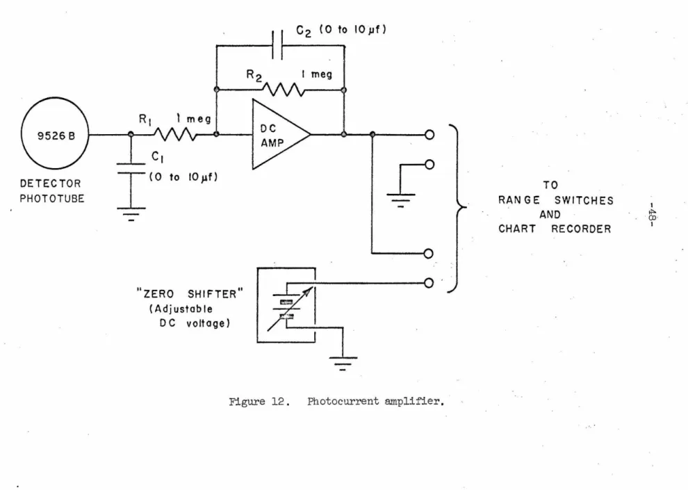
The signal from the detector photomultiplier tube is

processed as shown in Figure 12. After passing through a low-pass

filter consisting of R

1 and

c

1, i t is amplified and filtered again by a chopper stabilized DC operational amplifier. The signal is then

displayed on a Bro~m chart recorder either directly or with a constant

DC voltage subtracted from i t so that smal l changes may be observed.

The time constants "l

=

~

c

₁ and ..

2

=

R2

c

2 of the two

low-pass filters are usually set at 5 or 10 seconds which, at the

scanning speed of 79.6 ~/min, provides the most noise filtration

without excessively smearing out the absorption lines being measured.

For strong lines where the signal-to-noise ratio is larger, smaller time constants are sometimes used.

DETECTOR PHOTOTUBE

C

2 ( 0 to I 0 J.1 f )

R2 I meg

R

₁

l

meg

C1

I(O

to 10 Jlf)

I'

II ZERO SHI FTER

11

(Adjustable

DC voltage)

Figure 12 . Photocurrent amplifier.

TO

RANGE SWITCH ES AND

CHART RECORDER

I

tJ:>.

OJ·

signals cover a large span on the chart recorder with the zero shifted

signal displayed at a magnification of up to 100 times compared to

the unshifted signal. This magnification is kno~m as the scale ratio.

While scanning a line the magnified signal i s normally recorded. To

record the continuum level, the recorder is switched t o the unshifted

signal for a few seconds. This may be done automatically either at

one minute intervals or whenever the scanning direction is reversed.

Figure 13 shows two examples of the recorded data. To

obtain the equivalent width a straight line is drawn connecting the

continuum on each side of the line and the area is measured with a

planimeter. The equivalent width is proportional to the area divided

by the continuum level and scale ratio.

The smallest equivalent widths which can be measured with

this apparatus are about 0.1

mR.

This is 2 to 3 times better than the

performance of the light chopping apparatus used by Lawrence and Link.

The improvement is due to the elimination of noise from irregularities

in the chopping process, better photoelectron statistics, and the fact

that the reference signal is taken closer to the wavelength being

100 80

PHOTOTU3C:

CURRENT 60 (Arbitrary uni ts) 40

20

I-

t-0

-CONTINUUM LEVEL "

(Sampled when scon direction is reversed)

). 3261

"V

CADMIUM RUN

Octol>er 19, 1966 Scan 20

Scale ratio 100: I Time constants: 5 sec

-100 0

>. -

Ao

100 200

<> (mA) 300 (a)

t

-400

(Sampled once

per minute l

"3247

w,. • 9.oo mit

-200 ). - Ao

COPPER RUN Morch 16, 1965

Seen 41

Scale ratio 5: I Time constants: I sec

0 200

Cm!>

(b)

Figure 13. Equivalent width recordings.

1 CJ1

0

IV DATA AND RESULTS

The procedure followed in obtaining the data is as follows: Values of the various quantities relating to the geometry

of the atomic beam are measured each time the furnace is assembled

for a run. From. these measurements Q is calculated using equation

(51). After the vacuum system has been pumped down, the furnace is

heated to produce an atomic beam and the phototubes are scanned back

and forth over the line to record data on equivalent vddths. Each scan takes about 5 minutes. During this time, the shutter under the

microbalance pan is opened for a few minutes to record the deposit

rate and recovery times, and the furnace temperature is measured.

After the line has been scanned several times, the furnace temperature

is changed and more scans are made. This is continued until data have

been obtained for as wide a range of atomic beam densities as possible. Usually 20 to 30 scans are recorded for eqch line.

For each scan, values of WA, G, tR' and T are obtained and

a value of f is calculated as described in Section II-I. A weight is assigned to each measurement depending on the slope of the curve of growth in the region -where the measurement was made and the apparent

quality of the equivalent vddth and deposit rate data. The f-value

is then calculated as the weighted mean of the individual measurements.

The experimental results are reported in the follm,dng

Sections along vd th a discussion of methods and problems unique t"o