Stated Preference Analysis of Driver Route Choice Reaction To Variable Message Sign Information

This is a repository copy of Stated Preference Analysis of Driver Route Choice Reaction To Variable Message Sign Information.

White Rose Research Online URL for this paper: http://eprints.whiterose.ac.uk/2114/

Monograph:

Wardman, M., Bonsall, P.W. and Shires, J. (1996) Stated Preference Analysis of Driver Route Choice Reaction To Variable Message Sign Information. Working Paper. Institute of Transport Studies, University of Leeds , Leeds, UK.

Working Paper 475

[email protected] https://eprints.whiterose.ac.uk/ Reuse

See Attached Takedown

If you consider content in White Rose Research Online to be in breach of UK law, please notify us by

White Rose Research Online http://eprints.whiterose.ac.uk/

Institute of Transport Studies University of Leeds

This is an ITS Working Paper produced and published by the University of Leeds. ITS Working Papers are intended to provide information and encourage discussion on a topic in advance of formal publication. They represent only the views of the authors, and do not necessarily reflect the views or approval of the sponsors.

White Rose Repository URL for this paper: http://eprints.whiterose.ac.uk/2114

Published paper

M. Wardman, P.W. Bonsall and J.D. Shires (1996) Stated Preference Analysis of Driver Route Choice Reaction To Variable Message Sign Information. Institute of Transport Studies, University of Leeds, Working Paper 475

UNIVERSITY OF LEEDS

Institute for Transport Studies

ITS

Working Paper

475

June 1996

Stated Preference Analysis of Driver Route Choice Reaction

To Variable Message Sign Information

M Wardman, PW Bonsall and

JD

shires

This work has been undertaken following the financial assistance of the Engineering and Physical Sciences Research Council via theirfunding of a rolling programme of research into Fundamental Aspects of Route Guidance.

Contents Page

Section Page Number

1. INTRODUCTION AND OBJECTIVES 2

2. BACKGROUND 2.1 Influencing Route Choice 2.2 The Stated Preference Approach

3. STATED PREFERENCE DESIGN & DATA COLLECTION 5

3.1 Design - _- 5

3.2 Data Collection 11

4. EMPIRICAL FINDINGS 4.1 Sample Characteristics 4.2 Modelling Issues 4.3 Model S t m m 4.4 Initial Models

4.4.1 The Linear Model

4.42 The Power Model

4.5 Summary of Results on The Impact of Different VMS Messages &Visible Delays

5. TRIP CHARACTENSTICS & SOCIO-ECONOMIC 23

SEGMENTATION

5.1 Modelling Approach

5.2 Segmentation by Time Constraint

5.3 Age Segmentation 5.4 Sex Segmentation

5.5 Segmentation by Frequency of Jomneys to Manchester 5.6 Segmentation by Familiarity With Alternative Routes 5.7 Segmentation by Fkperience of Variable Message Signs 5.8 Preferred Route Choice Model

6. FORECASTS OF THE EFFECT OF VMS MESSAGES ON USE 35

OF THE M62

7. CONCLUSIONS 7.1 General

7.2 Policy Implications

7.3 Methodological Considerations

ACKNOWLEDGEMENTS 41

REFERENCES 42

STATED PREFERENCE ANALYSIS OF DRIVER ROUTE CHOICE

REACTION TO VARIABLE MESSAGE SIGN INFORMATION

1.

INTRODUCTION AND OBJECTIVES

Highway Authorities in many parts of the world have, for some years, been using variable message panels mounted above or beside the camageway to communicate short messages to motorists. Most such applications have been concerned with hazard warning and speed advice. However, their use to deliberately affect route choice is an area of great current interest. It is recognised that they have a potential role in managing demand to match the capacity available, not only to alleviate acute problems caused by roadworks and accidents, but also to contribute to satisfactory performance of networks operating close to capacity over extended periods of high, but variable, demand.

The installation and operation of the panels is not cheap and there is a widespread belief that overuse, or inappropriate use, of

the

messages may lead to them losing their credibility with the motorists and thus ceasing to be effective. It is therefore very important to understand the likely response of motorists to various messages before displaying them and even before selecting sites for the installation of panels. A number of researchers have explored drivers' responses to traffic information and route advice offered via variable message signs (VMS). Evidence from traffic counts suggests that messages can persuade somewhere between 5% and 80% of drivers to divert. Clearly this range of estimates is far too wide to support the use of VMS for fine tuning the pattern of demand. A major contributor to the uncertainty, however, is the varying, and often unknown, proportion of drivers whose destination makes the message relevant to them. More detailed studies involving driver interviews downstream of the VM!3 site to determine the relevance of

the

message, as well as the response to it, include those by Kawashima (1991) and Durand-Raucher et al. (1993). These studies have produced more precise estimates of compliance but the results are obviously limited to those messages which were on display at the time the interviews were being conducted. A number of researchers have sought to overcome this restriction by examining response to a range of messages presented via a stated preference exercise (see for example Hato et al., 1995; Shao et al., 1995 and Bonsall and Whelm, 1995), via a route-choice-simulator (see for example Firmin, 1996; Bonsall and Merrall, 1995 ; Bonsall and Palmer, 1997) or via a full scale driving simulator or system mock-up (see for example Mast and Ballas, 1976 and Brocken and Van der Vlist, 1991).

This

research has suggested that response is highly dependent on message content, subjects' network knowledge, and on the extent of any implied diversion.

We see particular value in extending this earlier work to consider a wider range of messages and to determine whether the route-choice-simulator results can be repeated and extended using a somewhat cheaper methodology

-

namely stated preference analysis.

The objectives of the work reported in this paper were thus:

to construct explanatory models of drivers' route choice behaviour in response to a variety of messages

to explore the factors influencing this response

to compare these results with previous results obtained using a variety of data collection methods

to draw policy conclusions, where appropriate, on the use of variable message signs to influence drivers' route choice

to draw conclusions, where appropriate, on our data collection and modelling methodology.

2

BACKGROUND

2.1 Influencing Route Choice

Most operational models of network-scale route choice are based on the assumption that drivers are seeking to minimise a simple objective function such as travel time. Modellers' main efforts (as reviewed by Watling, 1994) have been directed towards adequate representation of aggregate equilibrium processes at work in the network rather than towards realistic representation of the dynamics of individual behaviour or the potential for influencing that behaviour.

The network assignment models in widespread use were designed to predict aggregate

link

flows, but we argue that

the

changing nature of highway planning, from essentially _- - reactive infrastruct&e provision to more proactive-syst~m management, makes it appropriate to pay more attention to the factors which might be used to influence individual route choice.

Previous studies, reviewed by Bonsall (1992), have identified a number of factors influencing individual route choice. They include: overall expected journey time (minimisation of); delays (avoidance of); congestion (avoidance of); signposted routes (adherence to); tolls (avoidance of); safety and security hazards (avoidance of); unfamiliar routes (avoidance of); and scenic quality (maximisation of). In our current work, we wish to explore the extent to which information about delays and congestion displayed on a variable message sign might influence route choice. We were particularly interested to determine the extent to which the detailed content of the message might influence the response and the extent to which

the

response is influenced or constrained by driver characteristics or network knowledge.

2.2 The Stated Preference Approach

Tnis study has made use of the Stated Preference (SP) technique in order to evaluate drivers' responses to information on road traffic conditions. Prior to discussing the design and analysis of

the

SP experiment, we here highlight the salient features of this method of examining travel behaviour.

An SP experiment offers decision makers (eg, individuals, groups, companies) a series of hypothetical scenarios to be evaluated, usually in the form of discrete choices between travel alternatives. The alternatives are characterised by variables whose effects on travel behaviour we wish to examine. A typical SP experiment involves between 9 and 16

The technique has its roots in consumer behaviour and marketing research (Green and Srinivasen, 1978) and has experienced widespread acceptance and application in transport research since the mid 1980's. It has been extensively applied to the analysis of mode choice, particularly for urban travel, but with a significant number of applications to motorists' route choices (Bradley et al., 1986; Hensher et al, 1990; Wardman, 1991; Brocken and Van der Vlist, 1991; Ortuzar et al., 1994). There are also numerous unpublished SP studies by consultants as a result of the recent increased interest in private sector financing of road schemes, particularly in Great Britain and Eastern Europe (TPA, 1990; Gibb, 1996; Halcrow Fox, 1995; Kocks et al., 1995; Mott MacDonald, 1996)

.

The

attractions of the SP approach largely stem from its ability to control the choice context and

the

independent variables that will enter the demand model. ZL;. summary, its principal advantages are:

i) It can avoid problems of collinearity between, and insufficient variation in, key variables of interest.

ii) It can be used where an actual choice context does not exist, for example, where tolled roads, road pricing or indeed variable message signs are absent.

iii) It can deal with situations beyond the range of current experiences, for example, somewhat higher car taxes for environmental reasons.

iv) Multiple choice observations canbe obtained per person, thereby redudng data collection costs for any level of precision.

The main shortcomings of

the

SP approach, and conversely

the

principal attraction of Revealed Preference (RP) models based on actual behaviour, are related to the fact that individuals are not committed to behave in accordance with their SP responses. Random error, such as might be expected as a result of misunderstanding, uncertainty, respondent fatigue and not taking

the

exercise seriously, will have implications for forecasting, although not for relative values which are derived as

the

ratios of coefficients, because the coefficients of choice models depend on the residual variation (Bates, 1988). Of greater concern, since it can affect the relative valuations as well as the scale of the

model, is error which is of a more systematic nature, such as

the

strategic biassing of responses in order to influence policy. The evidence in both respects is quite encouraging, since stated preferences have generally been found to correspond reasonably well with revealed preferences (Louviere et al., 1980; Hensher and Truong, 1983; Wardman, 1988,1991, Bradley and Gunn, 1990; Hensher, 1992; Ortuzar et al., 1994). However, it is widely recommended that, whenever possible, SP models are given some basis in actual behaviour, such as through the estimation of joint RP-SP models (Bradley and Daly, 1991).

3

STATED PREFERENCE DESIGN AND DATA COLLECTION

3.1 Design

Our

SP

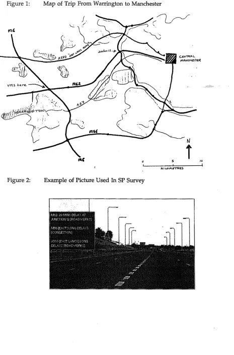
exercise was based on a trip of around 34km from Warrington to Manchester City Centre as depicted in Figure 1. This journey was chosen because it allowed the SP exercise to be based on the choice between four distinctly different routes which thereby allows a wider range of travel conditions and trade-offs between variables to be considered than in the binary choice context more typically used in

SP

exercises. Respondents, resident in Warrington, were asked to assume that they were travelling to Manchester City Centre on the M62 motorway (this being the natural route given the location of the survey) and that, as they approach the M62/M6 intersectiol~, they see a Vh4S panel displaying information on traffic conditions ahead.

A pictorial representation of the choice context was devised. As can be seen in figure 2, this comprised a photograph of the approach to the M62/M6 intersection, showing a 'through-the windscreen' view of traffic conditions on the M62 ahead and on the off- ramp leading to the M6 and a roadside VMS panel displaying a text message about traffic conditions ahead. This information was in the form of estimated delays on three of the four routes and the causes of those delays. The 'through the windscreen' information about current traffic conditions was reinforced with a written description of the traffic conditions at the site.

Respondents were asked to indicate which of the following routes they would use to complete their journey to central Manchester:

i continue via M62

ii divert via off-ramp to M6 northbound and thence via the A580 iii divert via off-ramp to M6 southbound and thence via the U56

iv divert via off-ramp to M6 southbound and thence via the A57

Note that the M62 and M56 routes provide grade separated routes to within a few kilometres of the destination while the A580 and A57 routes are of lower design standard, the A57 is the lowest quality route and includes several stretches through urban areas.

Respondents were expected to make a choice in the light of the photograph and reinforcing text. Thus they had available the following information:

-

_{local traffic conditions on the M62 ahead (queuing or clear)}

-

local traffic conditions on the off-ramp to

the

M6 (queuing or clear)

- _{expected delays ahead on specified routes (notified via the VMS panel - see}

Table 1, section c for list)

- _{cause of these delays (notified via the VMS panel - see Table 1, section d}

[image:9.595.47.513.63.768.2]

Figure 1: Map of Trip From Warrington to Manchester

1

k l I O r n r n E 5

MNL

HLl

FIGURE 3:

Possible

nested

structure

M62

A

M56 A580 A57

[image:10.595.63.568.17.812.2]

&

A57

FIGURE

4:

Alternative

structures

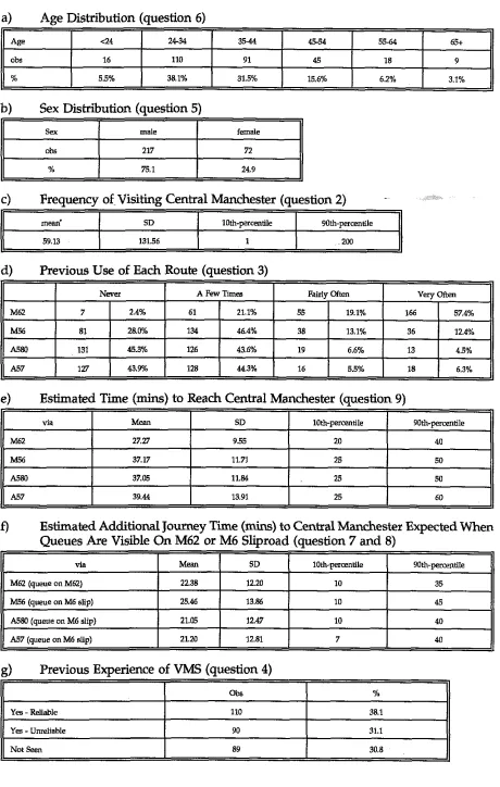
M62

In addition to this they will have had their own perception of the various alternative routes for reaching central Manchester from the M62/M6 intersection. Respondents were therefore asked to provide their own estimate of travel times to central Manchester via four specified routes. We can regard their estimates as being fairly well informed because 91% of our respondents had made at least one journey to central Manchester in the previous year and, for these, the average number of trips made was 53 (for further discussion of this point see later).

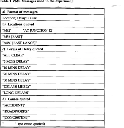
Table 1 VMS Messages used in the experiment

-

a) Format of messages

11

Location; Delay; Cause

b) Locations quoted

"M62 "AT JUNCTION 12

"M56 [EAST]"

"A580 [EAST LANCSY

11

C) Levels of Delav auoted

11

- -

11

"ALL CLEAR"

11

"5 MINS DELAY

11

--

11

"10 MINS DELAY "20 MINS DELAY

"30 MINS DELAY

11

"DELAYS LIKELY

11

11

"LONG DELAYS

I/

11

d) Causes quoted

11

"[ROADWORKS]"

"ICONGESTIONI"

U

8 8

' (no cause quoted)

[image:11.602.73.504.214.660.2]

An orthogonal fractional factorial SP design was used (Kocur et al., 1983) containing three variables at four levels and three variables at two levels. The three variables at two levels were: whether the M62 ahead is queuing or clear; whether the M6 slip road is queuing or clear and whether the journey is being made with a time constraint. The three variables at four levels relate to the information displayed on the roadside VMS about three possible routes

-

the M62, the A580 and the M56.

As can be seen from Table 1 section c the amount of delay was presented in terms of minutes or, in order to test the effectiveness of qualitative indicators of delay, as "delays likely" or "long delays" As can be seen from Table 1 section d, the design includes three causes of delay, "roadworks", "congestion" and "accident", with a fourth category where no reason was given.

This overall design was accommodated via the 16 sets of 8 questions outlined in Table 2. Note that sets 1-8 differ from sets 9-16 only in that the former included mention of the time constraint in the preamble while the latter did not). In devising this design we had the following concerns:

(1) to ask each respondent no more than 8 SP questions, (so as to minimise response fatigue effects);

(2) not to mix messages which offered no cause for the delay with those that did (to have done so might have caused some confusion and engendered complex patterns of assumed causes);

(3) to ensure that the M62 route was usually penalised more heavily than the others (because it would otherwise have dominated the choices);

(4) to emphasise, in any one set of questions, a range of delay levels rather than a

range of causes (in order to simplify the respondents' task); and

(5) to avoid unrealistic combinations of information (thus we replaced rather artificial

"5 MINS DELAY [ A C C I D W by "ALL CLEAR)

In order to test whether the overall design was satisfactory, in the sense of allowing the accurate estimation of the values of the variables in

the

design, simulation tests were conducted using synthetic route choice data which mimics how rational individuals might choose (Fowkes and Wardman, 1988). The results of this simulation exercise showed that the designs were capable of supporting the analysis we wished to undertake.

3.2 Data Collection

Prior to the main survey, a pilot survey was conducted in July 1995. Questionnaires were delivered to households in North East Warrington near to the M62 but no contact was made with residents. The responses obtained did not indicate any problems with the SP exercise but the response rate of 8.6% was very low. A contributory factor here was that the survey was conducted in the first week of the school summer holidays, and some residents would have been on holiday, whilst other households contacted would not have a car. In addition, it was felt that the absence of any personal contact and attempt

to obtain the co-operation of the householder was a significant shortcoming. We therefore subsequently adopted an approach whereby the survey staff called at homes and the questionnaires were personally handed to residents with cars available. Respondents were told about the purpose of the survey and advised that it did not matter it they had

not made a recent trip to Manchester to guard against non-response on this account. Of the 900 questionnaires which were handed out, 314 were returned giving a response rate

of 34.9% which is typical of this surveying method. Adding the questionnaires from the

pilot survey gives a total sample of 357 individuals. The data set available for modelling purposes removes those who have not fully completed the questionnaire and contains

289 individuals and a total of 2304 choice observations.

4

EMPIRICAL FINDINGS

4.1 Sample Characteristics

Table 3 shows the respondents' characteristics as revealed in their answers to the questionnaire.

4.2 Modelling Issues

The SP experiment offered choices between four routes. The most straightforward means of analysing discrete route choice is to calibrate a m u l t i n o d logit (MNL) model which expresses the probability (P) that an individual i chooses some alternative j as a function of the utilities (U) of the m alternatives in the choice set:

In turn, the utility for any alternative j is related to relevant variables representing individuals' travel situations

(4)

and socio-economic characteristics (Si):

uv

= f(cr/Xlp8rS,) (2)

Table 3: Respondents' Characteristics

b) Sex Distribution (question 5)

I1 11

a) Age Distribution (question 6)

Age

obs

%

II

d) Previous Use of Each Route (question 3)

I

<24

16

5.5%

Sex

c) Frequency of Visiting Central Manchester (question 2)

mwn' 2434 110 38.1%

II

male

e) Estimated Time (mins) to Reach Central Manchester (question 9)

g) Previous Experience of VMS (question 4)

I, I

female

SD

via

f) Estimated Additional Journey Time (mins) to Central Manchester Expected When

Queues Are Visible On M62 or M6 Sliproad (question 7 and 8)

3544

91

31.5%

via

M62 (queue on M62)

M.56 (queue on M6 slip)

A580 (queue on M6 slip)

A57 (queue an M6 slip)

10th-percenale

59 13

Mean

Yes - Reliable

Yer -Unreliable

Not Seen

4544

45

15.6%

90th-percenhle

131.56 1

Mean 22.38 25.46 21.05 21.20 2W SD M62 110 90 89 55-64 18 6.2%

27.27 955

SD 12.20 13.86 12.47 12.81 38.1 31.1 30.8 65t 9 3.1%

10th-percentile 90th-percentile

[image:16.605.74.534.53.777.2]

The main limitation of the

MNL

model is its so-called independence of irrelevant alternatives property (Luce and Suppes 1965) which stems from Ihe assumption that the unobserved influences on choice which are contained in

the

model's error term have - a common variance and are uncorrelated across alternatives. The result of this is that, say, a n increase in delays on the M62 will be forecast to increase demand on each of the other three routes by the same proportionate amount. In other words, a property of the MNL model is that

the

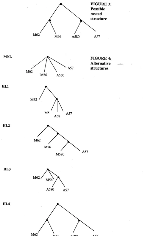
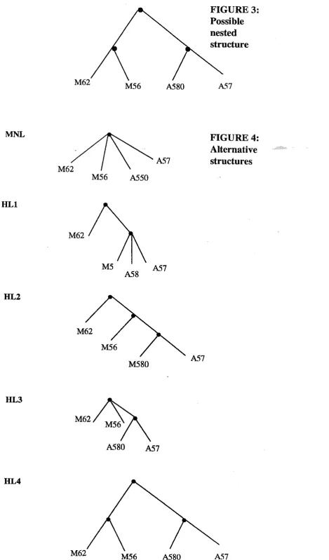
cross-elasticities are equal. The most common and straightforward means of allowing for possible different rates of substitutability between travel alternatives is to use the hierarchical logit model. This model adopts a 'nesting' structure which we can illustrate with an example.

We have four routes, two of which are motorways (M62 and M56) and two of which are A roads (A57 and A580). If the motorways have common unobserved influences and the A roads also have common unobserved influences, we would wish to 'nest' the routes as shown in figure 3. The upper nest consists of a composite motorway route and a composite A road route. The utility of a composite route is represented by its expected maximum utility (EMU) and also those variables (Z) which are

the

same for each of the component routes. Thus

the

utility for the composite motorway route

)

,

,

U

,

(

would be:

where:

[image:18.595.68.538.22.822.2]

FIGURE

3:

Possible

nested

structure

M62

A

M56 A580 A57

MNL

4

M7

FIGURE 4:

Alternative

structures

M62

4.3 Model Structure

We have examined the following five model structures which are depicted in Figure 4.

i) Multinominal Logit Model (MNL)

ii) Hierarchical Logit Model (HLl), with an upper nest of M62 against all other routes and a lower nest containing the three other routes which each involve using the off-ramp.

iii) A generalisation of ii) whereby its lower nest is further disagregated. The upper nest therefore contains M62 against all other routes, the middle nest contains the M56 against the A roads and the lower nest contains the two A roads (HL2).

iv) Hierarchical logit model (HL3) with the upper nest containing the M62 motorway, the M56 motorway and a composite A-road alternative, and the lower nest containing the two A-roads.

v) Hierarchical logit model (HL4) with the upper nest containing two composite alternatives relating to motorways and A roads.

Of these, HL.3 performed marginally better than the others. This is interpreted as indicating that the two A-roads (A580 and A57) are perceived as having more in common with each other than with either of the motorways and that the two motorways have less in common with each other than do the two A-roads. We suggest that the A-

road similarity is associated with design standards and frequent opportunities to exit while the motorway dissimilarity is due to one being the "straight-on" option while the other implies a significant diversion.

In the current study, we wished to explore a wide range of variables and a considerable number of disaggregations. This would put our data set under considerable pressure were we to adopt a hierarchical structure because the latter requires separate coefficients to be estimated for any variable which enters different nests and this is the case for many variables. Thus given that HL3 performed only marginally better than the multinomial logit model, and that its 0 parameter was in any event little different to the value of one whereby HL3 would collapse to the multinomial form, we have decided to proceed with the multinomial structure.

4.4 Initial Models

Likely and Long are dummy variables, as is the variable (Clear) which denotes whether

the sign indicated that the M56 was clear. The models also contain variables representing the normally expected travel time on each route (Time) and the amount of extra time that

the respondent thought would be incurred on each route if queuing was visible on the relevant slip road (Vis-Q). This latter formulation provided a somewhat better fit than

simply spedfying dummy variables for whether there was queuing or not. Three route specific constants (RSC's) were included (RSCm,, RSC,,, RSC,,).

The reported Rho-Squared figure (pf) is defined with regard to the log-likelihood of a constants only model and this is lower than

the

measure defined with respect to chance but the latter is strongly dependent upon the share of each alternative in the sample.

The difference between the two models reported in Table 5 is in terms of tbc frmctional form of the delay variable. What we have termed the 'power model' enters delay time

(D)

in a form that allows the unit value of delay time to vary with the amount of delay. Such a utility function takes the form:

If h exceeds one, the unit value of delay time increases with the amount of delay time whereas the value falls as delay time increases when his less than one. The linear model is obtained when his constrained to equal one and this functional form characterises the vast majority of logit model applications in transport research.

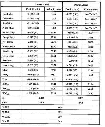
There are a number of desirable features of the models reported in Table 5. It can be seen that all the estimated coefficients have the correct sign and are statistically sigruficant even at a 1% level. The goodness of fit is high for models based on SF data, with values nearer to 0.1 being typical of the more common mode choice applications, although mode specific SP exercises tend to perform better in this respect because there are fewer extraneous influences. The reported values are in units of time (in minutes) and are generally plausible. They are marginal values calculated as the ratio of the derivative of the utility function with respect to the variable in question and the derivative of the

[image:21.595.68.506.100.625.2]

Table 5: Initial Models

4.4.1 The Linear Model

where Var and Cov denote variance and covariance. Table 6 contains 6 comparisons of the delay coefficients, 6 comparisons of the Likely coefficients and 6 comparisons of the

-

-Long coefficients according to the cause of

the

delay. In addition, it presents comparisons of the estimated delay coefficients with the estimated time coefficient and comparisons

of the -Likely and -Long coefficients for each cause of delay.

The results indicate that our respondents are most sensitive to additional delav when its stated cause is an accident. The t statistics presented in Table 6 show that the Acc-Mins

coefficient estimate is statistically significantly different from the three other delay coefficient estimates even at a 1% level of significance. This finding is consistent with that reported by Bonsall and Merrall (1995) and by Bonsall and Palmer (1995) and is believed to reflect the acute nature of delays due to accidents. None-Mins has the lowest

coefficient and it is significantly different in two of the three comparisons at the usual 5% level of significance and almost significantly different in the remaining case. This suggests that additional delay has the least influence on route choice when no cause is stated. Again, this result is very much in line with findings from previous work. Cong-

Mins and Road-Mins were estimated to have very similar values.

As can be seen from Table 5,

the

disutility of additional delay time quoted by the VMS exceeds that of normal journey time for all four causes of delay, with the ratios varying between 1.30 and 1.70 and three of the four coefficients being significantly different from the time coefficient. Delay time might be expected to be more highly valued than journey time due to the uncertainty, stress, frustration and the worse driving conditions involved, although the extent to which motorists consider that the amount of delay time quoted by the VMS is likely to be an overestimate (underestimate) will obviously cause the delay coefficients to be lower (higher) than if delays are interpreted with certainty. It is worth noting that a number of earlier studies have found congestion related delay time to be valued more highly than free flow time. Wardman (1991) found the relative values of

.

'delay' and 'free flow' travel time to be 1.43 while Oscar Faber TPA (1992) obtained a value of 1.39. Hensher et a1 (1990) obtained more variable results, with ratios of 1.7 for commuters in company cars and approximately 1.0 for other journey purposes. Note that the current study specified the source of the information as VMS and, for many

What the VMS presented as "likely delays" are valued at between 10 and 31 minutes of normally expected travel time, depending on the stated cause of the delay. Again, it is the specification of "accident" as the cause of the delay which has the largest impact and the Acc-Likely coefficient estimate is significantly different from the coefficients for Road-

Likely and Nme-Likely at the 5% level.

The

value of delay is again relatively low when no cause is specified with the Nme-Likely estimate significantly lower than the Acc-Likely and Cmg-Likely estimates. This finding reflects previous work by Bonsall and Merall, 1995 and Bonsall and Palmer, 1995. It is notable that the Road-Likely coefficient is relatively low; the evidence from the other two dimensions would lead us to expect it to be similar to the Cong-Likely coefficient. The relative ineffectiveness of a "Roadworks Likely" message has been observed in other studies and it is speculated that the reason may be a widespread belief that highway authorities more, in an attempt to persuade drivers to keep clear of their roadworks, may take advantage of tb inherent uncheckability of a "Delays Likely" message to say that delays are likely at roadworks even when they are not.

The

implied values of "long delays" vary between 35 and 47 minutes of normally expected journey time depending on the stated cause. In all four cases, these coefficients are meater than those for the equivalent "likely delays" and in two cases the difference is statistically significant with

a

further difference -almost significant. It is again the accident cause which has the biggest imuact on choice. However, there are no simificant _" differences between the Long cGfficient estimates.

A VMS message indicating that a route is "all clear" (a message which was in fact specific to the M56) has a different effect on choice than does a blank VMS indicating nothing

about road conditions. It has a valuation equivalent to 9.90 minutes of normal journey

time. Tnis is presumably because the respondents' estimates of normal journey time included an element of delay time.

The value of Vis-Q was estimated by using each respondent's stated expectation of delays due to visible queues on the M62 and the off-ramp. Somewhat to our surprise, the results suggest that Vis-Q is valued at only half that of normal travel time. Reasons that might be advanced to explain this finding are:

i) Notwithstanding the phrasing of the question, respondents have reported worst case additional delay times arising from visible delays rather than mean values;

ii) There is a tendency to ignore the visible effects when VMS information is presented;

iii) Respondents are unable to make reliable estimates of delays to be expected when queues are visible;

iv) An unwanted correlation in our design between VIS-Q and delay;

v) Respondents have put less weight on the visible delays in the SP exercise then they would in an actual choice situation.

respondents to use worst case estimates in part of the questionnaire but means in another.

In order to gather evidence on the second reason, dummy variable interaction terms were used to allow the Vis-Q coefficient to vary according to whether VMS information was provided. The incremental effect indicated that more notice was indeed taken of visible delays when no VMS messages were provided. This effect was also apparent in another study (Bonsall and et al., 1995) and is interpreted as representing the fact that VMS information about conditions ahead is, in some senses, a substitute for visible information about current conditions. However, in the current study the effect was far from statistically significant (t=0.6).

With regard to the third reason, the M56, A580 and A57 all have the same off-ramp and, although they do not have to possess

the

same expected delays as a result of visible queuing, we would not expect the differences across these routes to be particularly large.

Examination of the data showed that although the differences in the means were small (see Table 3.0 there was no clear pattern in the delays expected via the different routes and there were very appreciable mean absolute differences between the delays expected on the M56 and the A580 and on the M56 and the A57 (8.92 minutes and 10.09 minutes respectively). These figures seem rather large and raise concerns about the reliability of this data. However, it is unlikely that unreliable delay times can provide the whole explanation, particularly since the estimated value of Vis-Q is so much lower than the value of normal time whereas we would have expected it to be more highly valued.

With regard to the fourth reason, examination of the correlation matrix showed that the highest correlation of estimated coefficients involving Vis-Q was 0.23 with cong-mins

,

and thus we are confident that correlation will not have caused any problems here. We must therefore conclude that there is an element of respondents failing to fully account for the visible delays in their SP choice process.

4.4.2 The Power Model

We now turn to the issue of

the

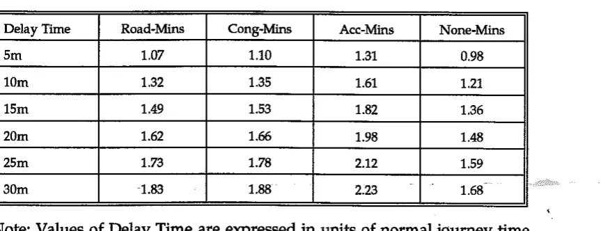
functional form of delay time in the utility expression, that is, the power model. We are not in a position to simultaneously estimate both a and

h of equation 6. Instead, we examine a range of prespecified values of h and select the

model which provides the best fit. For simplicity we have constrained h to be the same

regardless of the cause of the delay. The value of h which provided the best fit was 1.3,

which improved the goodness of fit statistic (p:) from 0.184 to 0.189.

Table 7: Values of Delay Time from Power Model (h = 1.3)

Note: Values of Delay Time are expressed in units of normal journey time.

Comparison of the linear and power models presented in Table 5 lead us to conclude that the new model is to be preferred.

4.5 Summary of Results on the Impact of Different VMS Messages and Visible Delays

We have seen that the impact of expected delays on route choice varies with the specified cause of

the

delay, that delay time is valued more highly than expected travel time, and that

the

value of delay time is quite sensitive to the amount of delay time with increasing sensitivity as delay time increases. The results suggest that VMS messages can have a significant impact on traffic flows, an issue which we shall return to in section 6.

Although the ordering of the impacts of the four causes of delay does vary, we can conclude that

the

accident cause has the largest impact whilst not specifying a reason tends to lead to relatively low values. This seems plausible given the

high

level of uncertainty that inherently surrounds accidents. It may also be that motorists regard VMS messages relating to delays due to an accident as having more inherent credibility than

ones which mention roadworks or which offer no cause at all. Motorists may believe that the traffic authorities might mention delays on VMS signs in order to influence traffic flow in ways that would not necessarily benefit

the

individual traveller but that the message can be trusted if accidents are mentioned. Whatever the reason, the findings that messages mentioning accidents are more persuasive than ones mentioning roadworks or giving no cause at all is consistent with earlier findings.

[image:26.595.76.508.102.268.2]

5 TRIP CHARACTERISTICS AND SOCIO-ECONOMIC SEGMENTATION

We now explore the extent to which results differ according to the characteristics of the trip and the personal characteristics of the respondents. The variables which we have examined within our preferred model form (multinomial logit model with power function of delay time) are:

i) Whether there was a binding arrival time constraint ii) The age of the respondent

iii) The sex of the respondent

iv) The frequency of respondents' trips between Warrington and ivlanchester v) Respondents' familiarity with

the

alternative routes

vi) Respondents' prior experience of variable message signs

5.1 Modelling Approach

The approach we have adopted specifies dummy variable interaction terms to allow the coefficients to vary across different categories of relevant characteristics. To do this, we specify dummy variables for n-1 of n categories and create interaction terms as the product of the dummy variables and the independent variables. To illustrate the method, let us specify a simple utility function containing a single independent variable (X):

If we wish to examine whether the coefficients of the utility function vary across

the

n categories of some segmentation variable, we specify the utility function as:

where Dj, is a dummy variable denoting whether an individual or trip is in a particular category. Thus the effect on utility from variable X would comprise two terms for all except the omitted (n'th) category.

Although we can specify more than one segmentation in a single model (MVA et al.,

1987), we initially estimated models which contained only a single segmentation in order to identify the principal sources of variation in coefficients which could then be taken forward to a more complete model.

The following sections present the results of our investigations of each potential segmentation and conclude as to whether it ought to be taken forward to our final, complete, model.

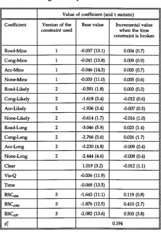
5.2 Segmentation by Time Constraint

Just over half (51%) of respondents were asked to imagine that their journey to Central Manchester involved a time constraint in the form of having to drop someow ~ f f for an appointment 45 minutes after passing the roadside sign. The remainder of the sample were given no instructions regarding arrival time constraints.

It is hypothesised that motorists will be more sensitive to delays if there is a risk that they might miss their appoihtment. We therefore constructed a variable which, for each route, denoted whether the VMS delay time in minutes would cause the time constraint

to be broken. An alternative specification allowed, not only for whether

the

constraint was broken, but also for the extent to which it was broken given the expected journey time on that route and any delays due to visible queues. This latter specification gave a slightly better fit, its prease formulation is given in equation (10).

(journey

time +VlS-Q+delay-45) x delay, if

journey

time

+VIS-Q+delay > 45

...

₍₁₀₎

Given the unquantified nature of "Delays Likely" and "Long delays", we cannot construct an equivalent measure of the extent to which these variables would lead to the arrival time constraint being broken. However, it is reasonable to expect the likelihood that such a qualitative delay will be perceived to break the time constraint to increase the higher the respondents' expected journey time. We therefore specified the time constraint variable for

the

unquantified delays as in equation (11).

(journey

time +VlS-Q+delay-45) x delay, if

journey

time +VIS-Q+delay > 45

...

₍₁₁₎

This variable provided the basis of the segmentation of the Likely and

Long

coefficients and provided a slightly better fit than simply segmenting the coefficients by whether a

time constraint was specified or not.

The

route specific constants were segmented simply according to whether a time constraint was specified or not.

Table 8: Model Segmented by Time Constraint

constraint use when the time

constraint is broken

Definition of time constraint variables:

1 Dummy x expression in equation (10)

2 Dummy x expression in equation (11)

3 Dummy

Where dummy = 1 if time constraint is specified

[image:29.595.71.397.106.580.2]

problems. Any feeling that motorways are inherently more susceptible to unavoidable delays may have been unwittingly reinforced by our experiment having shown the worst problems on the M62 and never having mentioned any on the A57. If this explanation were valid is perhaps conceivable that an 'avoid motorways' effect outweighs the expected incremental effect on the delay coefficients. On balance, however, we do no feel sufficiently confident in this explanation to warrant including time constraint variables in our preferred model.

5.3 Age Segmentation

We conducted a simple segmentation by age, according to whether the individual was less than 35, on the basis that additional age categories could be specified if h e simple segmentation proved successful. The results are presented in Table 9, section A.

There seems to be a general tendency for the incremental effect of being under 35 to moderate the value of the base coefficient

-

that is for the young respondents to be less sensitive to the specified attributes than are other people. In only one case (Vis-Q) is this effect statistically significant but it is certainly worthy of note because it is consistent with evidence from previous work (e.g. Bonsall and Joint 1992) in suggesting that young people are less inclined to comply with

V M S

advice.

In order to test whether the younger respondents' relative insensitivity to delay information becomes significant when only one incremental effect is sought for all levels of delay, we specified a more parsimonious model where the incremental effects on the delay time coefficients were constrained to be the same across all four causes of delay and the segmentation on Vis-Q was maintained.

Table 9: Models Segmented by Age

A

Road-Mins

1

-0.039 (11.0)

1

0.006 (1.2)

1

-0.039 (14.1)

1

B

II

effect if

Age < 35

Base

effect if Age c 35

Cong-Mins Acc-Mins None-Mins

I

Cong-Likely ACC-Likely None-Likelv Incremental

-0.039 (11.0) -0.047 (11.8)

-0.033 (9.1)

Road-Long

Cong-Long

ACC-Long

None-Long

5.4 Sex Segmentation

-2.021 (3.8) -2.081 (3.9) -0.793 (2.0)

Clear

Vis-Q

Time

The results of the segmentation by sex are given in Table 10 and the findings are similar to the age segmentation with the general model (A) showing a limited effect on the delay time coefficients. The subsequent model (B) which constrains the incremental effects to be the same across the four causes of delay obtains a statistically significant effect which indicates that the females (25%) in

the

sample are less sensitive to delay time. Again this finding is consistent with the results of previous studies (Bonsall, 1992b; Conquest et al., 1993; Khattak et al., 1993; Mamering et al., 1994; Bonsall and Merrall, 1995; Emmerink et al., 1996) which found female drivers less willing to divert from their initially determined route.

Base

0.005 (0.8) 0.007 (1.3) 0.009 (1.0)

-2.490 (5.8) -1.928 (5.4) -3.527 (4.9) -2.878 (4.8)

Incremental

0.413 (0.6) 0.041 (0.1) -0.121 (0.3)

1.085 (4.1) -0.042 (11.3) -0.075 (11.1)

-0.040 (14.4)

-0.046 (15.3) -0.034 (12.0)

-0.364 (0.5) -1384 (1.7) 0.587 (0.6) 0.614 (0.8)

0.0047 (2.5)

-1.811 (5.0) -2.059 (5.1) -0.851 (2.9)

-0.603 (1.5) 0.013 (2.2) 0.006 (0.6)

n / a

n/a

n / a

-2.653 (8.0) -2.365 (7.5) -3.224 (7.0) -2.573 (6.4)

n/a

n/a

n/a

n/a

0.811 (4.2) -0.042 (11.6) -0.072 (14.3)

n / a

0.014 (2.5)

[image:31.595.63.503.103.621.2]

Table 10: Model Segmented by Sex A Cong-Long Acc-Long Base B None-Long

5.5 Segmentation by Frequency of journeys to Manchester

Incremental effect if

Female

Base

-2.274 (6.5)

3.504 (5.9)

Vis-Q

Time

RSC,,

We segmented respondents according to the frequency with which they had visited Manchester on the basis that this might capture effects relating to familiarity with the routes in question, (a more precise specification of familiarity with each route is considered in section 5.6). Frequency of trip making might proxy for the respondent's information on general driving conditions and hence on how visible queues and messages specifying likely and long delays would be interpreted. A number of different frequency thresholds were tested and the one which proved most effective was five trips per year (15 versus >6). 36% of our total sample fell into the low frequency category thus defined. The results in Table 11 reveal that the principal effect of frequency of trip making is on the route specific constants and on Vis-Q. The Vis-Q coefficient is lower for infrequent travellers which is consistent with the idea that respondents lacking good local

Incremental effect if

Female

1

0.786 (3.5)

1

0.224 (0.5)

1

0.809 (4.2) n/a -2.592 (6.0)

-0.426 (0.5)

0.845 (0.9)

-0.040 (12.3)

-0.078 (13.2)

-1.554 (10.9)

-0.004 (0.1)

-2.363 (8.0)

-3.222 (7.0)

-2.589 (6.5)

0.014 (2.1)

0.020 (1.1)

0.012 (0.1)

n/a

n/a

-0.037 (13.2)

-0.072 (14.4)

-1.551 (12.8)

n/a

n/a

[image:32.595.67.497.100.552.2]

knowledge would be less able to appreaate the signtficance of visible queues at the M62/M6 intersection.

Table 11: Model Segmented by Frequency of Journeys to Manchester

We note a tendency, albeit not statistically significant, for the infrequent drivers to put less weight on the VMS estimates of delay; suggesting perhaps that they do not feel as

[image:33.602.73.500.135.583.2]

Vis-Q incremental effect forward to our preferred model. Table 11, section B shows that, when this is the only incremental effect of infrequency, its effect is to reduce the value of Vis-Q by 30%.

5.6 Segmentation by Familiarity with Alternative Routes

Previous research, for example by Mahmassani and Chen (1991), Bonsall and Joint (1991) and Hato et al. (1995), has suggested that familiarity with a network is likely to reduce the desire to comply with directional guidance whilst increasing the ability to respond to traffic information. It might thus be expected that

the

willingness of motorists to switch from the natural route to Manchester (the M62), and hence their sensitivity to delays, would depend on their familiarity with the alternative routes. We asked respondents how often they had used each route to Manchester, with permissible responses being "very often", "fairly often", "a few times" and "never". Almost everyone (98%) had used the M62 to Central Manchester with 76% having used it fairly often or very often We defined a dummy variable ('unfamiliar') as being true for a respondent if they said they had never used two of the alternative routes and had used the third a few times at most. This criterion resulted in 30% of our sample being defined as unfamiliar with the alternative routes. It can be seen in Table 12 that no clear or strong effects have emerged from this unfamiliarity segmentation. This may reflect the complexity of any familiarity effect as noted in previous research.

[image:34.595.71.349.368.781.2]

An alternative specification was to allow the RSCs to depend on whether the respondent had ever used that route (on the grounds that, all other things equal, a respondent is less likely to choose a route with which he is completely unfamiliar). The proportions stating that they had never used the M56, A580 and A57 routes to Manchester were 28%, 45% and 43%, in contrast to only 2% for the M62. Table 13 shows that those who had never used the route in question are less likely to choose it; for example, the (negative) constant for the A57 is 73% greater for those who have never used it. This finding is highly significant.

We also examined additional incremental effects for each constant where respondents had only used a route a few times but the coefficients were far from significant. Nor was

the extension of this segmentation to the delay time coefficients successful.

Table 13: Segmentation of Constants by 'Never Used' the Each Route

- Road-Mins Cong-Mins ACC-Mins None-Mins Road-Likely Cong-Likely Acc-Likely None-Likely Road-Long Cong-Long Acc-Long None-Long Clear Vis-Q Time

R % m

RSc.4580

R s c ~ 7

P:

Base

-0.037 (14.3)

-0.039 (14.8)

-0.044 (15.4)

-0.033 (11.9)

-0.587 (2.5)

-1.878 (5.2)

2 . ~ 0 (5.1) -0.826 (2.8)

-2.736 (8.2)

-2.442 (7.7)

3.337 (7.2)

-2.588 (6.5)

0.821 (4.2)

-0.037 (13.2)

-0.067 (13.4)

-1.495 (11.8)

-1.338 (10.5)

-1.462 (11.0)

Incremental Effect if Unfamiliar With Alternatives

-0.548 (3.8)

-0.958 (6.7)

-1.070 (9.2)

[image:35.602.72.397.290.700.2]

5.7 Segmentation by Experience of Variable Message Signs

Previous research, for example by Bonsall and Joint (1991), Janssen and Van der Horst (1992), Hato et al. (1995) and Zhao et al. (1995), has demonstrated that compliance with diversion advice is highly dependant on the credibility of that advice as judged from its previous record of reliability. We therefore asked individuals whether they had ever seen an electronic variable message roadside sign and whether they had found them to be a reliable guide to conditions ahead. 39% stated that they had seen such signs and found them to be reliable, 31% had found them to be unreliable and 30% stated that they had not seen one. Table 14 reports results of segmentation which examine whether there is an impact on the coefficients from perceived unreliability and whether variable message signs had ever been seen.

Table 14: Model Segmented by Experience of Variable Message Signs

[image:36.595.70.448.295.698.2]

coefficient estimate, obtained when the incremental effects were constrained to be the same for all four cause of delay, was also insignificant (t=1.3). Not having seen an electronic roadside variable message sign does not have any impacts which approach statistical significance.

The only significant effect is that respondents who have found

V M S

unreliable have a greater weight on their Vis-Q coefficient. This is obviously very plausible on the grounds

that those who find

V M S

unreliable will take more notice of visible queues. The reason why we have not discerned any effects from unreliability on the VMS messages may well be because some respondents interpreted unreliability to mean the VMS understated delays, others interpreted it to mean that VMS overstated delays whilst yet others may

have interpreted unreliability as a random effect. Unfortunately, we did not enquire as to what individuals interpreted unreliability to mean. Table 15 reports a model which maintains only the effect of unreliable VMS messages on the Vis-Q coefficient. The latter

is 50% higher for those who find VMS to be unreliable.

[image:37.595.68.351.319.747.2]

5.8 Preferred Route Choice Model

Our preferred overall model is a multinomial logit formulation with a power term for the delay time and contains all the segmentation variables that have been identified as significant and plausible in the preceding sections. The model is presented in Table 16 and it can be seen that, with the exception of

the

effect of sex on the delay coefficients which is now somewhat lower, the incremental effects are little different to those obtained in

the

separate models and all the effects retain their statistical significance. A likelihood ratio test' comparing our preferred model with the power model in Table 5 which does not contain any segmentation variables yields a

xZ

of 162.4 which, given a tabulated

x2

value of 20.09 for 8 degrees of freedom, indicates that the segmented model is statistically superior even at a 1% level of sigruficance.

Table 16: Preferred Overall Model

Age c 35 0 . W (2.2)

Female 0.0040 (2.0)

Note: The delay time in minutes variables are all raised to the power 1.3 as in the power model of Table 5.

[image:38.599.68.509.224.681.2]

Table 17 shows the incremental effects in proportionate terms. Although the proportionate effects of age and sex are not particularly large, the other effects are appreciable.

Table 17: Proportionate Incremental Effects

Perhaps the main disappointment with respect to the segmentation analysis, apart from the failure to obtain an effect from applying a time constraint, is that we have not been able to detect variations in the Likely and Long coefficients according to socio-economic or network familiarity factors. We believe that this is, at least in part, due to different interpretations by different respondents of the amount of implied delay time. This will have lead to essentially random variations in the Likely and Long coefficients across individuals and this will of course have made it more difficult to discern variation in coefficients due to differences in socio-economic or network familiarity factors.

With the benefit of hindsight, we should have asked respondents what they considered the likely delays and long delays to mean in terms of extra minutes delay for each of the causes of delay. This would have reduced the coefficient variation across individuals to just that which might arise because individuals have different valuations of any given level of delay. For example, it is noticeable that when we changed from a dummy variable specification of whether queues were visible to one that entered the respondents' perceived amounts of delay associated with visible queues, the goodness of fit increased quite appreciably from 0.169 to 0.193.

6

FORECASTS OF THE EFFECT OF VMS MESSAGES ON USE OF

THE M62

Finally, we use our preferred overall model, outlined in Table 16, to illustrate the effect that various VMS messages and visible queues can have on traffic flows. We are here using our model to make predictions for the situation in which it has been calibrated where there are three good alternatives to the most natural route. In other sets of circumstances the number of alternative routes and the extent to which they are close

[image:39.595.71.507.173.319.2]

by displaying VMS messages will be much less than we are predicting for the Warrington-Manchester example.

The forecasting procedure is based on the sample enumeration approach, that is, choice probabilities are obtained for each of

the

289 individuals in our sample and these are summed to obtain overall market shares. The base situation uses only the reported journey times for each route along with the route specific constants and incremental effects as appropriate. This yields market shares for the M62, M56, A580 and A57 of 76.7%, 8.5%, 8.3% and 6.5% respectively.

The

natural route to Central Manchester in this context would be the M62 and a larger share than 76.7% might have been expected for the base situation. This discrepancy may be associated with the fact that our model is calibrated against the postulated background of unusually severe problems s:-L

the

M62

and this may have caused

the

RSCs for the other routes to be more favourable than would normally be expected. This problem is overcome by using the model in incremental form - thus avoiding use of RSCs. An alternative reason for the discrepancy could be the so called 'scale-factor problem' (Wardman, 1991), whereby systematic bias in the coefficient is associated with an inappropriate residual error in the SP model. The recommended means of overcoming

the

scale-factor problem is to rescale the model using observed data. Unfortunately we do not have access to such data.

It is normal practice, when faced with a model which does not properly replicate base market shares, to rescale the model using observed data (on the assumption that the error is due to systematic error in

the

SP

responses). We do not have any observed data with which to perform such an operation and so will concentrate our attention on predicted changes to relative market shares rather than on absolute values.

We now present three sets of forecasts according to the nature of the delay variable and allowing for

the

socio-economic and familiarity effects appropriate for each variable. We have reported both a revised share for

the

M62 and the proportionate change in demand (in brackets) resulting from changes in

the

circumstances relating to the M62.

Table 18: Forecasts of Effects of Delay Time on Proportion Using M62

C

AU

NO Delays @lase) 5m Delay - Accident

10m Delay - Accident

2 h Delay - Accldent

30m Delay - Accldent

5m Deiay - No R-n

Femk 76.69 69.9 (-9%) 58.4 (-24%)

10m Delay - No Reason

Table 19 presents forecasts of the effects of the qualitative indicators of delay on the number using the M62. Again it can be seen that there is a dramatic effect, with a message of long delays due to accidents reducing the M62 share by 84%.

29 0 (-62%) 8 6 (-89%) 71 8 (-6%)

20m Delay - No Reason

3Om Delay - No Reason

Table 19: Forecasts of Effects of 'Qualitative' Factors on Proportion Using M62

Male

n . 0

70.9 (-8%) 60.6 (-21%) 63.8 (-17%) 33 2 (-57%) 115 (-85%) 72.8 (-6%) 415 (-a%) 19.8 (-74%)

Table 20 shows the impact of changes in visible delays and provides forecasts for the segmentation for which significant variation in the Vis-(2 coefficient was discerned. Forecasts are provided for situations where each individual perceives delays of 20 minutes and 30 minutes due to visible queues and also for the level of delay time which

Age<% 76.6 69.6 (-9%) 57.7 (-25%) 65.8 (-15%) -

No Delays (Base)

Likely Delays - Roadworks

Likely Delays - Congestion

Likely Delays - Accident

Likely Delays

-

No Reason

Long Delays - Roadworks

Long Delays

-

Congestion

Long Delays

-

Accident

Long Delays

-

No Reason

All Clear M56

Asem 27.6 (-64%) 7.7 (-90%) 715 (-7%) 46.3 (4%) 252 (-67%) Overall 76.7 65.2 (-15%) 36.0 (-53%) 31.2 (-59%) 59.9 (-22%) 19.9 (-74%)

24.6 (48%)

12.2 (-84%)

21 h (-72%)

69.6 (-9%) 76.3 69.8 (-9%) 59.0 (-23%) 63.1 (-18%)

n . 0

70.0 (-9%) 58.0 (-2.570) 30 9 (-60%) 10 1 (-67%) 64.3

(-16%) (-18%)

[image:41.602.72.507.89.345.2] [image:41.602.73.306.443.664.2]

each individual reported that they associated with visible delays on the M62. Even though we believe that the estimated Vis-Q coefficient understates

the

impact of visible queues, the results in Table 20 show that route choice is sensitive to delays that the individual perceives as a result of observing queuing. There is also appreciable variation in the impact across the different segmentation categories.

Table 20: Effect of Changes in Visible Delays on Proportion Using M62

Finally, we address two issues concerned with the constants in our preferred model. The effect of the 'nmer use' incremental coefficient is seen to be quite important: if we assume that none of

the

sample had ever used routes other

than

the M62, then the M62 share is predicted to increase from 76.7% to 85.0%, whereas if all the sample had used all the alternative routes at least once, the share is predicted to fall to 71.9%. Clearly, the transferability of the absolute values of our predictions is constrained by the presence of constants specific to our routes. However, this problem can be overcome by using the model in incremental form (Kumar, 1980). For example, Table 21 shows results for four hypothetical cases where a motorway is in competition with one other route with differing levels of base market share. Notice the sensitivity of

the

predicted share to the message even where the motorway was initially very dominant.

Table 21: Effect of

VMS

messages on use of motorways with various levels of base market shares

Base Motonvay Share

80%

60%

50%

33%

Motonvay Share When "10

MINUTE DELAY is displayed

62%

38%

29%

17%

Motorway Share When "20

MINUTE ACCIDENT DELAY is Displayed

27%

12%

8%

[image:42.595.67.560.200.372.2] [image:42.595.67.528.578.735.2]

7.

CONCLUSIONS

7.1 General

It can be expected that motorists will consider changing routes, when they have the opportunity to do so, if their expectations of traffic conditions ahead are amended due to changes in the information available to them. This could arise due to roadside variable message signs (VMS), observation of traffic conditions immediately ahead or in-car information systems such as RDS/TMC dedicated messages, autonomous in-car guidance devices or even conventional radio messages.

The research reported in this paper has examined the impact on route choicc ~f changes in information occurring as a result of roadside VMS, including a comparison of the relative effectiveness of quantitative and qualitative descriptions of delay, and 'through the windscreen' observation.

Although the effects of information on route choice behaviour will vary according to the number of alternative routes that are available and the extent to which they are close substitutes, and the analysis reported here was based on a situation of four closely compekg routes, our results show that route choice can be strongly influenced by the provision at appropriate points of information on traffic conditions ahead. In addition to

this

overall effect, a number of other interesting findings emerged.

Additional delays mentioned on the VMS panel have been found to be valued more highly than normally expected travel time with ratios, from our linear model, between 1.30 and 1.70 depending on the stated cause of the delay. These values are consistent with other evidence of which we are aware. The high value presumably reflects the greater stress, frustration and unreliability of driving in conditions where delays are present.

Qualitative descriptions of delays were found to be able to have an appreciable impact on route choice. "Long delays" were valued at between 35 and 47 minutes depending on the stated cause while "delays likely" were valued at between 10 and 31 minutes

-

again depending on the stated cause.

It was apparent that the unit value of expected delay time increases as the amount of delay time increases, at least within the range of delay times offered in this study. The

variation in the value of delay time between 5 and 30 minutes is considerable.

It was found that different stated causes of delay had different impacts. Delays attributed to accidents have the biggest impact on route choice whilst if no cause was

quoted the messages have a relatively low effect. These findings are consistent with evidence from other sources.