https://doi.org/10.5194/bg-15-5891-2018 © Author(s) 2018. This work is distributed under the Creative Commons Attribution 4.0 License.
An intercomparison of oceanic methane and nitrous
oxide measurements
Samuel T. Wilson1, Hermann W. Bange2, Damian L. Arévalo-Martínez2, Jonathan Barnes3, Alberto V. Borges4, Ian Brown5, John L. Bullister6, Macarena Burgos1,7, David W. Capelle8, Michael Casso9, Mercedes de la Paz10,a, Laura Farías11, Lindsay Fenwick8, Sara Ferrón1, Gerardo Garcia11, Michael Glockzin12, David M. Karl1, Annette Kock2, Sarah Laperriere13, Cliff S. Law14,15, Cara C. Manning8, Andrew Marriner14,
Jukka-Pekka Myllykangas16, John W. Pohlman9, Andrew P. Rees5, Alyson E. Santoro13, Philippe D. Tortell8, Robert C. Upstill-Goddard3, David P. Wisegarver6, Gui-Ling Zhang17, and Gregor Rehder12
1University of Hawai’i at Manoa, Daniel K. Inouye Center for Microbial Oceanography: Research and Education (C-MORE),
Honolulu, Hawai’i, USA
2GEOMAR Helmholtz Centre for Ocean Research Kiel, Düsternbrooker Weg 20, 24105 Kiel, Germany 3Newcastle University, School of Natural and Environmental Sciences, Newcastle upon Tyne, UK 4Université de Liège, Unité d’Océanographie Chimique, Liège, Belgium
5Plymouth Marine Laboratory, Plymouth, UK
6National Oceanic and Atmospheric Administration, Pacific Marine Environmental Laboratory, Seattle, Washington, USA 7Universidad de Cádiz, Instituto de Investigaciones Marinas, Departmento Química-Física, Cádiz, Spain
8University of British Columbia, Department of Earth, Ocean and Atmospheric Sciences, British Columbia,
Vancouver, Canada
9U.S. Geological Survey, Woods Hole Coastal and Marine Science Center, Woods Hole, USA 10Instituto de Investigaciones Marinas, Vigo, Spain
11University of Concepción, Department of Oceanography and Center for climate research and resilience (CR2),
Concepción, Chile
12Leibniz Institute for Baltic Sea Research Warnemünde, Rostock, Germany
13University of California Santa Barbara, Department of Ecology, Evolution, and Marine Biology, Santa Barbara, USA 14National Institute of Water and Atmospheric Research (NIWA), Wellington, New Zealand
15Department of Chemistry, University of Otago, Dunedin, New Zealand
16University of Helsinki, Department of Environmental Sciences, Helsinki, Finland
17University of China, Key Laboratory of Marine Chemistry Theory and Technology (MOE), Qingdao, China acurrent address: Instituto Español de Oceanografía, Centro Oceanográfico de A Coruña, A Coruña, Spain
Correspondence:Samuel T. Wilson ([email protected]) Received: 10 June 2018 – Discussion started: 14 June 2018
Revised: 10 September 2018 – Accepted: 14 September 2018 – Published: 5 October 2018
Abstract.Large-scale climatic forcing is impacting oceanic biogeochemical cycles and is expected to influence the water-column distribution of trace gases, including methane and nitrous oxide. Our ability as a scientific community to eval-uate changes in the water-column inventories of methane and nitrous oxide depends largely on our capacity to ob-tain robust and accurate concentration measurements that can be validated across different laboratory groups. This study
derive the dissolved gas concentrations were also evaluated for inconsistencies (e.g., pressure and temperature correc-tions, solubility constants). The results from the intercom-parison and intercalibration provided invaluable insights into methane and nitrous oxide measurements. It was observed that analyses of seawater samples with the lowest concen-trations of methane and nitrous oxide had the lowest preci-sions. In comparison, while the analytical precision for sam-ples with the highest concentrations of trace gases was better, the variability between the different laboratories was higher: 36 % for methane and 27 % for nitrous oxide. In addition, the comparison of different batches of seawater samples with methane and nitrous oxide concentrations that ranged over an order of magnitude revealed the ramifications of different calibration procedures for each trace gas. Finally, this study builds upon the intercomparison results to develop recom-mendations for improving oceanic methane and nitrous oxide measurements, with the aim of precluding future analytical discrepancies between laboratories.
1 Introduction
The increasing mole fractions of greenhouse gases in the Earth’s atmosphere are causing long-term climate change with unknown future consequences. Two greenhouse gases, methane and nitrous oxide, together contribute approxi-mately 23 % of total radiative forcing attributed to well-mixed greenhouse gases (Myhre et al., 2013). It is imper-ative that the monitoring of methane and nitrous oxide in the Earth’s atmosphere is accompanied by measurements at the Earth’s surface to better inform the sources and sinks of these climatically important trace gases. This includes mea-surements of dissolved methane and nitrous oxide in the ma-rine environment, which is an overall source of both gases to the overlying atmosphere (Nevison et al., 1995; Anderson et al., 2010; Naqvi et al., 2010; Freing et al., 2012; Ciais et al., 2014).
Oceanic measurements of methane and nitrous oxide are conducted as part of established time series locations, along hydrographic survey lines, and during disparate oceano-graphic expeditions. Within low-latitude to midlatitude re-gions of the open ocean, the surface waters are frequently slightly supersaturated with respect to atmospheric equilib-rium for both methane and nitrous oxide. There is typically an order of magnitude range in concentration along a ver-tical water-column profile at any particular open ocean lo-cation (e.g., Wilson et al., 2017). In contrast to the open ocean, nearshore environments that are subject to river in-puts, coastal upwelling, benthic exchange, and other pro-cesses have higher concentrations and greater spatial and temporal heterogeneity (e.g., Schmale et al., 2010; Upstill-Goddard and Barnes, 2016).
Methods for quantifying dissolved methane and nitrous oxide have evolved and somewhat diverged since the first measurements were made in the 1960s (Craig and Gordon, 1963; Atkinson and Richards, 1967). Some laboratories em-ploy purge-and-trap methods for extracting and concentrat-ing the gases prior to their analysis (e.g., Zhang et al., 2004; Bullister and Wisegarver, 2008; Capelle et al., 2015; Wil-son et al., 2017). Others equilibrate a seawater sample with an overlying headspace gas and inject a fixed volume of the gaseous phase into a gas analyzer (e.g., Upstill-Goddard et al., 1996; Walter et al., 2005; Farías et al., 2009). The purge-and-trap technique is typically more sensitive by 1– 2 orders of magnitude over headspace equilibrium (Magen et al., 2014; Wilson et al., 2017). However, the purge-and-trap technique requires more time for sample analysis and it is more difficult to automate the injection of samples into the gas analyzer. Headspace equilibrium sampling is most suited for volatile compounds that can be efficiently parti-tioned into the headspace gas volume from the seawater sam-ple. To compensate for its limited sensitivity, a large vol-ume of seawater can be equilibrated (e.g., Upstill-Goddard et al., 1996). Additional developments for continuous under-way surface seawater measurements use equilibrator systems of various designs coupled to a variety of detectors (e.g., Weiss et al., 1992; Butler et al., 1989; Gülzow et al., 2011; Arévalo-Martínez et al., 2013). Determining the level of an-alytical comparability between different laboratories for dis-crete samples of methane and nitrous oxide is an important step towards improved comprehensive global assessments. Such intercomparison exercises are critical to determining the spatial and temporal variability of methane and nitrous oxide across the world oceans with confidence, since no sin-gle laboratory can sinsin-gle-handedly provide all the required measurements at sufficient resolution. Previous comparative exercises have been conducted for other trace gases, e.g., car-bon dioxide, dimethylsulfide, and sulfur hexafluoride (Dick-son et al., 2007; Bullister and Tanhua, 2010; Swan et al., 2014), and for trace elements (Cutter, 2013). These exercises confirm the value of the intercomparison concept.
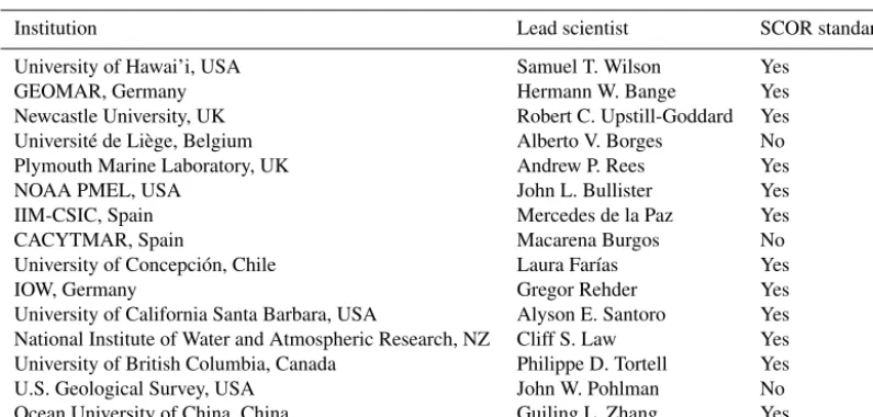
Table 1.List of laboratories that participated in the intercomparison. All laboratories measured both methane and nitrous oxide except the U.S. Geological Survey (methane only), UC Santa Barbara (nitrous oxide only), and NOAA PMEL (nitrous oxide from the Pacific Ocean). Also indicated are the 12 laboratories that received the SCOR gas standards of methane and nitrous oxide.
Institution Lead scientist SCOR standards
University of Hawai’i, USA Samuel T. Wilson Yes
GEOMAR, Germany Hermann W. Bange Yes
Newcastle University, UK Robert C. Upstill-Goddard Yes
Université de Liège, Belgium Alberto V. Borges No
Plymouth Marine Laboratory, UK Andrew P. Rees Yes
NOAA PMEL, USA John L. Bullister Yes
IIM-CSIC, Spain Mercedes de la Paz Yes
CACYTMAR, Spain Macarena Burgos No
University of Concepción, Chile Laura Farías Yes
IOW, Germany Gregor Rehder Yes
University of California Santa Barbara, USA Alyson E. Santoro Yes National Institute of Water and Atmospheric Research, NZ Cliff S. Law Yes University of British Columbia, Canada Philippe D. Tortell Yes
U.S. Geological Survey, USA John W. Pohlman No
Ocean University of China, China Guiling L. Zhang Yes
Q1 What is the agreement between the SCOR gas standards and the “in-house” gas standards used by each labora-tory?
Q2 How do measured values of dissolved methane and ni-trous oxide compare across laboratories?
Q3 Despite the use of different analytical systems, are there general recommendations to reduce uncertainty in the accuracy and precision of methane and nitrous oxide measurements?
Q4 What are the implications of interlaboratory differences for determining the spatial and temporal variability of methane and nitrous oxide in the oceans?
2 Methods
2.1 Calibration of nitrous oxide and methane using compressed gas standards
Laboratory-based measurements of oceanic methane and ni-trous oxide require separation of the dissolved gas from the aqueous phase, with the analysis conducted on the gaseous phase. Calibration of the analytical instrumentation used to quantify the concentration of methane and nitrous oxide is nearly always conducted using compressed gas standards, the specifics of which vary between laboratories. Therefore, the reporting of methane and nitrous oxide datasets ought to be accompanied by a description of the standards used, includ-ing their methane and nitrous oxide mole fractions, the de-clared accuracies, and the composition of their balance or “makeup” gas. For both gases, the highest-accuracy com-mercially available standards have mole fractions close to
current-day atmospheric values. These standards can be ob-tained from national agencies including the National Oceanic and Atmospheric Administration Global Monitoring Divi-sion (NOAA GMD), the National Institute of Metrology China, and the Central Analytical Laboratories of the Euro-pean Integrated Carbon Observation System Research Infras-tructure (ICOS-RI). By comparison, it is more difficult to ob-tain highly accurate methane and nitrous oxide gas standards with mole fractions exceeding modern-day atmospheric val-ues. This is particularly problematic for nitrous oxide due to the nonlinearity of the widely used electron capture detector (ECD) (Butler and Elkins, 1991).
uncer-tainty of the nitrous oxide mole fraction in the WRS was es-timated at 2 %–3 %. The gas standards were distributed to 12 of the laboratories involved in this study (Table 1). The technical details on the production of the gas standards and their assigned absolute mole fractions are included in Bullis-ter et al. (2016).
2.2 Collection of discrete samples of nitrous oxide and methane
Dissolved methane and nitrous oxide samples for the inter-comparison exercise were collected from the subtropical Pa-cific Ocean and the Baltic Sea. PaPa-cific samples were ob-tained on 28 November 2013 and 24 February 2017 from the Hawai’i Ocean Time-series (HOT) long-term monitoring site, station ALOHA, located at 22.75◦N, 158.00◦W. The November 2013 samples are included in Figs. S1 and S2 in the Supplement, but are not discussed in the main Results or Discussion because fewer laboratories were involved in the initial intercomparison, and the results from these samples support the same conclusions obtained with the more recent sample collections. Seawater was collected using Niskin-like bottles designed by John Bullister (NOAA PMEL), which help minimize the contamination of trace gases, in partic-ular chlorofluorocarbons and sulfur hexafluoride (Bullister and Wisegarver, 2008). The bottles were attached to a rosette with a conductivity–temperature–depth (CTD) package. Sea-water was collected from two depths: 700 and 25 m, at which the near maximum and minimum water-column concentra-tions for methane and nitrous oxide at this location can be found. The 25 m samples were always well within the surface mixed layer, which ranged from 100 to 130 m of depth dur-ing sampldur-ing. Replicate samples were collected from each bottle, with one replicate reserved for analysis at the Uni-versity of Hawai’i to evaluate variability between sampling bottles. Seawater was dispensed from the Niskin-like bottles using Tygon® tubing into the bottom of borosilicate glass bottles, allowing for the overflow of at least two sample vol-umes and ensuring the absence of bubbles. Most sample bot-tles were 240 mL in size and were sealed with no headspace using butyl rubber stoppers and aluminum crimp seals. A few laboratory groups requested smaller crimp-sealed glass bot-tles ranging from 20–120 mL in volume and two laboratories used 1 L glass bottles, which were closed with a glass stop-per and sealed with Apiezon®grease. Seawater samples were collected in quadruplicate for each laboratory. All samples were preserved using saturated mercuric chloride solution (100 µL of saturated mercuric chloride solution per 100 mL of seawater sample) and stored in the dark at room tempera-ture until shipment. The choice of mercuric chloride as the preservative for dissolved methane and nitrous oxide was due to its long history of usage. It is recognized that other preservatives have been proposed (e.g., Magen et al., 2014; Bussmann et al., 2015); however, pending a community-wide evaluation of their effectiveness over a range of microbial
as-semblages and environmental conditions for both methane and nitrous oxide, it is not evident that they are a superior alternative to mercuric chloride.
Samples from the western Baltic Sea were collected dur-ing 15–21 October 2016 onboard the R/VElisabeth Mann Borgese (Table 2). Since the Baltic Sea consists of differ-ent basins with varying concdiffer-entrations of oxygen beneath permanent haloclines (Schmale et al., 2010), a larger range of water-column methane and nitrous oxide concentrations were accessible for interlaboratory comparison compared to station ALOHA. For all seven Baltic Sea stations, the wa-ter column was sampled into an on-deck 1000 L wawa-ter tank that was subsequently subsampled into discrete sample bot-tles. At three stations (BAL1, BAL3, and BAL6), the wa-ter tank was filled from the shipboard high-throughput un-derway seawater system. For deeper water-column sampling at the stations BAL2, BAL4, and BAL5, the water tank was filled using a pumping CTD system (Strady et al., 2008) with a flow rate of 6 L min−1and a total pumping time of approx-imately 3 h. For the final deep water-column station, BAL7, the pump that supplied the shipboard underway system was lowered to a depth of 21 m to facilitate a shorter pumping time of approximately 20 min. Subsampling the water tank for all samples took approximately 1 h in total and the total sampling volume was less than 100 L. To verify the homo-geneity of the seawater during the sampling process, the first and last samples collected from the water tank were analyzed by Newcastle University onboard the research vessel. In con-trast to the Pacific Ocean sampling, which predominantly used 240 mL glass vials, each laboratory provided their own preferred vials and stoppers for the Baltic Sea samples. Sea-water samples were collected in triplicate for each labora-tory. All samples were preserved with 100 µL of saturated mercuric chloride solution per 100 mL of seawater sample, with the exception of samples collected by the U.S. Geologi-cal Survey, which analyzed unpreserved samples onboard the research vessel.
2.3 Sample analysis
Each laboratory measured dissolved methane and nitrous ox-ide slightly differently. A full description of each laboratory’s method can be found in Tables S6 and S7 in the Supplement for methane and nitrous oxide, respectively.
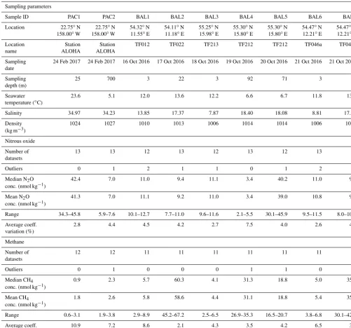
Table 2.Pertinent information for each batch of methane and nitrous oxide samples. This includes contextual hydrographic information, median and mean concentrations of methane and nitrous oxide, range, number of outliers, and the overall average coefficient of variation (%).
Sampling parameters
Sample ID PAC1 PAC2 BAL1 BAL2 BAL3 BAL4 BAL5 BAL6 BAL7
Location 22.75◦N 22.75◦N 54.32◦N 54.11◦N 55.25◦N 55.30◦N 55.30◦N 54.47◦N 54.47◦N 158.00◦W 158.00◦W 11.55◦E 11.18◦E 15.98◦E 15.80◦E 15.80◦E 12.21◦E 12.21◦E
Location Station Station TF012 TF022 TF213 TF212 TF212 TF046a TF046a
name ALOHA ALOHA
Sampling 24 Feb 2017 24 Feb 2017 16 Oct 2016 17 Oct 2016 18 Oct 2016 19 Oct 2016 20 Oct 2016 21 Oct 2016 21 Oct 2016 date
Sampling 25 700 3 22 3 92 71 3 21
depth (m)
Seawater 23.6 5.1 12.0 13.6 12.2 6.6 6.7 11.8 13.4
temperature (◦C)
Salinity 34.97 34.23 13.85 17.37 7.87 18.40 18.08 8.81 17.65
Density 1024 1027 1010 1013 1006 1014 1014 1006 1013
(kg m−3) Nitrous oxide
Number of 13 13 12 13 12 13 12 13 12
datasets
Outliers 0 1 2 1 1 0 1 2 2
Median N2O 42.4 7.0 11.0 9.4 11.1 3.4 40.2 11.0 9.6
conc. (nmol kg−1)
Mean N2O 41.3 7.0 11.1 9.2 11.0 3.4 39.0 10.8 9.5
conc. (nmol kg−1)
Range 34.3–45.8 5.9–7.6 10.1–12.7 7.7–11.0 9.6–11.6 2.1–5.5 30.1–45.9 9.5–11.5 8.0–10.4
Average coeff. 2.8 4.4 4.5 4.2 2.7 7.5 4.0 2.6 4.4
variation (%) Methane
Number of 12 12 11 11 11 11 11 11 11
datasets
Outliers 0 1 0 0 0 1 1 0 0
Median CH4 0.9 2.3 5.7 60.3 4.1 31.3 18.8 5.0 35.2
conc. (nmol kg−1)
Mean CH4 1.8 2.6 5.8 58.6 4.4 31.1 18.8 5.4 35.4
conc. (nmol kg−1)
Range 0.6–3.1 1.9–3.8 2.9–8.9 45.2–67.2 2.5–6.5 26.9–35.3 16.5–20.7 3.8–6.8 30.1–42.1
Average coeff. 10.9 7.2 8.6 2.1 4.3 3.5 4.2 6.5 3.5
variation (%)
the vessel used to conduct the headspace equilibration ranged from 20 mL borosilicate glass vials to 1 L glass vials and sy-ringes used by Newcastle University and the U.S. Geological Survey, respectively. The dissolved gases equilibrated with the overlying headspace at a controlled temperature for a set period of time that ranged from 20 min to 24 h for the dif-ferent laboratories. The longer equilibration times are due to overnight equilibrations in water baths. The majority of lab-oratories enhanced the equilibration process by some initial period of physical agitation. After equilibration, an aliquot
The final gas concentrations using the headspace equili-bration method were calculated by
Cgas[nmol L−1] =
βxP Vwp+
xP
RTVhs Vwp, (1)
whereβis the Bunsen solubility of nitrous oxide (Weiss and Price, 1980) or methane (Wiesenburg and Guinasso, 1979) in nmol L−1atm−1,xis the dry gas mole fraction (ppb) mea-sured in the headspace,P is the atmospheric pressure (atm),
Vwp is the volume of water sample (mL), Vhs is the
vol-ume (mL) of the created headspace, R is the gas constant (0.08205746 L atm K−1mol−1), and T is the equilibration temperature in Kelvin (K). An example calculation is pro-vided in Table S8 in the Supplement.
In contrast to the headspace equilibrium method, five lab-oratories used a purge-and-trap system for methane and/or nitrous oxide analysis (Tables S6 and S7 in the Supplement). These systems were directly coupled to a flame ionization detector (FID) or ECD, with the exception of the University of British Columbia, where a quadrupole mass spectrome-ter with an electron impact ion source and Faraday cup de-tector were used (Capelle et al., 2015). The purge-and-trap systems were broadly similar, each transferring the seawa-ter sample to a sparging chamber. Sparging times typically ranged from 5–10 min and the sparge gas was either high-purity helium or high-high-purity nitrogen. In addition to com-mercially available gas scrubbers, purification of the sparge gas was achieved by passing it through stainless steel tub-ing packed with Poropak Q and immersed in liquid nitrogen. This is a recommended precaution to consistently achieve a low blank signal of methane. The elutant gas was dried using Nafion or Drierite and subsequently cryotrapped on a sample loop packed with Porapak Q to aid the retention of methane and nitrous oxide. Cryotrapping was achieved for methane using liquid nitrogen (−195◦C) and either liquid nitrogen or cooled ethanol (−70◦C) for nitrous oxide. Subsequently, the valve was switched to inject mode and the sample loop was rapidly heated to transfer its contents onto the analyti-cal column. Calibration was achieved by injecting standards via sample loops using multi-port injection valves. The injec-tion of standards upstream of the sparge chamber allowed for calibration of the purge-and-trap gas-handling system, in ad-dition to the GA. Calculation of the gas concentrations using the purge-and-trap method was achieved by the application of the ideal gas law to the standard gas measurements:
P V =nRT , (2)
whereP,R, andT are the same as Eq. (1),V represents the volume of gas injected (L), and nrepresents moles of gas injected. Rearranging Eq. (2) yields the number of moles of methane or nitrous oxide gas for each sample loop injection of compressed gas standards. These values were used to de-termine a calibration curve based on the measured peak areas of the injected standards and thereafter derive the number of
moles measured for each unknown sample. To calculate con-centrations of methane or nitrous oxide in a water sample, the number of moles measured was divided by the volume (L) of seawater sample analyzed. An example calculation is provided in Table S8 in the Supplement.
2.4 Data analysis
The final concentrations of methane and nitrous oxide are re-ported in nmol kg−1. The analytical precision for each batch of samples obtained by each of the individual laboratories was estimated from the analysis of replicate seawater sam-ples and reported as the coefficient of variation (%). The val-ues reported by each laboratory for all the batches of seawa-ter samples are shown in Tables S1 to S4 in the Supplement. Due to the observed interlaboratory variability, it is likely that the median value of methane and nitrous oxide for each batch of samples does not represent the absolute in situ concen-tration. As this complicates the analytical accuracy for each laboratory, we instead calculated the percentage difference between the median concentration determined for each set of samples and the mean value reported by an individual lab-oratory. The presence of outliers was established using the interquartile range (IQR) and by comparing with 1 standard deviation applied to the overall median value.
3 Results
3.1 Comparison of methane and nitrous oxide gas standards
Six laboratories compared their existing “in-house” stan-dards of methane with the SCOR stanstan-dards. This was done by calibrating in-house standards and deriving a mixing ra-tio for the SCOR standards, which were treated as unknowns. Four laboratories reported methane values for either the ARS or WRS within 3 % of their absolute concentration, whereas two laboratories reported an offset of 6 % and 10 % between their in-house standards and the SCOR standards (Table S6 in the Supplement). For those laboratories who measured the SCOR standards to within 3 % or better accuracy, observed offsets in methane concentrations from the overall median cannot be due to the calibration gas.
frac-Figure 1.Concentrations of methane measured in nine separate seawater samples collected from the Pacific Ocean(a, b)and the Baltic Sea(c, d, e). The dashed grey line represents the value of methane at atmospheric equilibrium(b). Individual data points are plotted sequentially by increasing value. The same color symbol is used for each laboratory in all plots.
tion of the standard exceeded the signal typically measured from in-house standards or acquired by sample analysis by an order of magnitude. The high mole fraction of the WRS was not an issue when multiple sample loops of varying sizes were incorporated into the analytical system, which was the case for purge-and-trap-based designs. For the two laborato-ries with an in-house standard of comparable mole fraction to the WRS, an offset of 3 % and a>20 % offset were reported. 3.2 Methane concentrations in the intercomparison
samples
Overall, median methane concentrations in seawater samples collected from the Pacific Ocean and the Baltic Sea ranged from 0.9 to 60.3 nmol kg−1 (Table 2). Out of 101 reported
values, 3 outliers were identified using the IQR criterion and were not included in further analysis. The methane data val-ues for each batch of samples analyzed by each laboratory, including the mean and standard deviation, the number of samples analyzed, and the percent of offset from the overall median value, are reported in Tables S1 and S2 in the Sup-plement. Analysis conducted by the University of Hawai’i of
methane and nitrous oxide from each Niskin-like bottle used in the Pacific Ocean sampling did not reveal any bottle-to-bottle differences. Furthermore, analysis by Newcastle Uni-versity showed there was no difference between the first and the last set of samples collected from the 1000 L collection used in the Baltic Sea sampling.
The two Pacific Ocean sampling sites had the lowest water-column concentrations of methane (Fig. 1a and b). The PAC1 samples collected from within the mesopelagic zone, where methane concentrations have been reported to be less than 1 nmol kg−1(Reeburgh, 2007; Wilson et al., 2017),
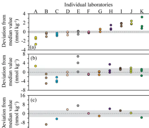
[image:7.612.138.457.69.388.2]Figure 2. Deviation from the median methane concentration (re-ported as absolute values in nmol kg−1) for the seven Baltic Sea samples. The batches of seawater samples: BAL1, BAL3, and BAL6 (a); BAL4, BAL5, and BAL7(b); BAL2 (c). The shaded grey area indicates values≤5 % of the median concentration. The color scheme for each laboratory dataset is identical to that used in Fig. 1 and the letters allocated to each dataset are to facilitate cross-referencing in the text. Note that theyaxis scale varies between the figures.
also had a distribution of data skewed towards the higher con-centrations.
Three Baltic Sea sampling sites (BAL1, BAL3, and BAL6) had median methane concentrations that ranged from 4.1 to 5.7 nmol kg−1(Fig. 1c). The BAL1 samples also showed a skewed distribution of reported values towards higher con-centrations, as seen in PAC1 and PAC2 samples. However, this was not evident in BAL3 or BAL6, which had the closest agreement between the reported methane concentrations. For these three sets of Baltic Sea samples, the mean coefficient of variation for all laboratories ranged from 4 % (BAL3) to 9 % (BAL1). The next three Baltic Sea samples (BAL4, BAL5, and BAL7) had methane concentrations that ranged from 18.8 to 35.4 nmol kg−1 (Fig. 1d). These three sets of sam-ples had a normal distribution of data and the closest agree-ment between the reported concentrations for all of the Pa-cific Ocean and Baltic Sea samples. Furthermore, for these three sets of samples, the mean coefficient of variation for all laboratories was 4 % (Table 2). The final Baltic Sea sample (BAL2) had the highest concentrations of methane, with a median reported value of 60.3 nmol kg−1 and a large range of values (45.2 to 67.2 nmol kg−1; Fig. 1e). The BAL2 sam-ples had the lowest overall mean coefficient of variation for all laboratories: 2 % (Table 2).
Further analysis of the data was conducted to better com-prehend the factors that caused the observed interlaboratory
variability in methane measurements. The deviation from median values was calculated for each sample collected from the Baltic Sea (Fig. 2). The Pacific Ocean samples (PAC1 and PAC2) were not included in this analysis due to the skewed distribution of data. There were also some instances in the Baltic Sea samples for which the median concentra-tion might not have realistically represented the absolute in situ methane concentration. This was most likely to have oc-curred at low concentrations due to the skewed distribution of reported concentrations (e.g., BAL1) or at high concen-trations for which there was a large range in reported val-ues (e.g., BAL2). The results revealed that a few laboratories (Datasets D, F, and G) were consistently within or close to 5 % of the median value for all batches of seawater samples (Fig. 2). Some laboratories (e.g., Datasets B, C, and H) had a higher deviation from the median value at higher methane concentrations. Two laboratories (Datasets J and K) had a higher deviation from the median value at lower methane concentrations. Finally, in some cases it was not possible to determine a trend (Datasets A and E) due to the variability.
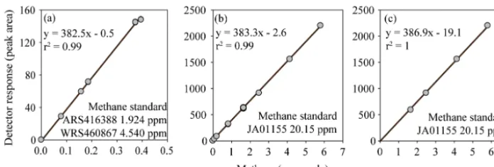
Figure 3.FID response to methane fitted with a linear regression calibration. The inclusion(a, b)or exclusion(c)of low methane values causes the calibration slope and intercept to vary. However, the observed variation in the calibration slope does not have a significant effect on the final calculated concentrations of methane. In contrast, variation in the intercept does have an effect on the final concentrations of methane.
3.3 Nitrous oxide concentrations in the intercomparison samples
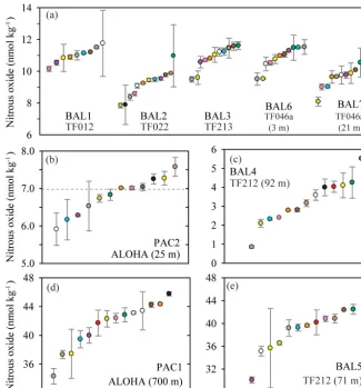
Overall, median nitrous oxide concentrations in seawater samples collected from the Pacific Ocean and the Baltic Sea ranged from 3.4 to 42.4 nmol kg−1(Table 2). Of the 113 re-ported values, 10 outliers were identified using the IQR cri-terion and were not included in further analysis. The nitrous oxide data values for each batch of samples analyzed by each laboratory, including the mean and standard deviation, the number of samples analyzed, and the percent of offset from the overall median value are reported in Tables S3 and S4 in the Supplement.
For six sets of seawater samples, BAL1, BAL2, BAL3, BAL6, BAL7, and PAC2, the concentrations of nitrous oxide were close to atmospheric equilibrium. The reported values ranged from 7.7 to 12.7 nmol kg−1in the Baltic Sea (Fig. 4a) and from 5.9 to 7.6 nmol kg−1in the Pacific Ocean (Fig. 4b). For the Pacific Ocean near-surface (mixed layer) sampling site (PAC2), the theoretical value of nitrous oxide concen-tration in equilibrium with the overlying atmosphere is also shown (Fig. 4b). For these six samples with concentrations close to atmospheric equilibrium, the mean coefficient of variation for all laboratories ranged from 3 % (BAL3 and PAC2) to 5 % (BAL1) (Table 2).
For the three other sets of samples (BAL4, BAL5, and PAC1), the nitrous oxide concentrations deviated signifi-cantly from atmospheric equilibrium (Fig. 4c, d, and e). At one sampling site, BAL4 (Fig. 4c), nitrous oxide was un-dersaturated with respect to atmospheric equilibrium and re-ported concentrations ranged from 2.1–5.5 nmol kg−1. As
observed in the low-concentration Pacific Ocean methane samples, there was a skewed distribution of the data towards the higher nitrous oxide concentrations. The BAL4 samples also had the highest variability (i.e., lowest precision), with a mean coefficient of variation of 8 % (Table 2). The two re-maining samples (PAC1 and BAL5) had much higher con-centrations of nitrous oxide, as expected for low-oxygen
re-gions of the water column. In contrast to the samples with near atmospheric equilibrium concentrations of nitrous ox-ide, there was a low overall agreement between the indepen-dent laboratories for PAC1 and BAL5 nitrous oxide concen-trations (Fig. 4d, e). At PAC1 and BAL5, nitrous oxide con-centrations ranged from 34.3–45.8 nmol kg−1 (Fig. 4d) and
30.1–45.9 nmol kg−1, respectively (Fig. 4e). The mean co-efficient of variation for all laboratories was 4 % for BAL5 samples compared to 3 % for PAC1 samples.
Figure 4.Concentrations of nitrous oxide measured in nine separate samples from the Baltic Sea and the Pacific Ocean. The dashed grey line represents the value of nitrous oxide at atmospheric equilibrium(b). Individual data points are plotted sequentially by increasing value. The same color symbol is used for each laboratory in all plots.
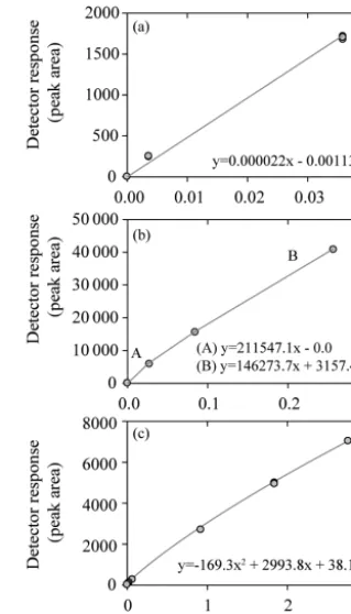
1991; Bange et al., 2001). The laboratories participating in the nitrous oxide intercomparison employed different cali-bration procedures (Fig. 6). Some used a linear fit and kept their analytical peak areas within a narrow range (Fig. 6a), while others used a stepwise linear fit and therefore used dif-ferent slopes for low and high nitrous oxide mole fractions (Fig. 6b). Finally, some applied a polynomial curve (Fig. 6c) and sometimes two different polynomial fits for low and high concentrations. The difficulty in calibrating the ECD was evidenced by the deviation from median values as multiple datasets show good precision but consistent offsets at the lowest (Fig. 5a) and highest (Fig. 5b) final concentrations of nitrous oxide.
3.4 Sample storage and sample bottle size
Because the prolonged storage of samples can influence dis-solved gas concentrations, including methane and nitrous oxide, the intercomparison dataset was analyzed for sam-ple storage effects (Table S5 in the Supsam-plement). It should,
however, be noted that assessing the effect of storage time on sample integrity was not a formal goal of the intercom-parison exercise and replicate samples were not analyzed at repeated intervals by independent laboratories, as would normally be required for a thorough analysis. Nonetheless our results did provide some insights into potential storage-related problems. Most notably, there were indications that an increase in storage time caused increased concentrations and increased variability for methane samples with low con-centrations, i.e., PAC1 and PAC2 samples, which had me-dian methane concentrations of 0.9 and 2.3 nmol kg−1, re-spectively (Fig. 7). In comparison, for samples of nitrous ox-ide with low concentrations there was no trend of increasing values as observed for samples with low methane concentra-tions.
Figure 5.Deviation from the median value (reported in absolute units) for nitrous oxide datasets. The batches of samples include BAL1, 2, 3, 6, and 7(a)and PAC2 and BAL5(b). The Baltic Sea samples are represented by circles and the Pacific Ocean samples are represented by triangles. The shaded area indicates a deviation ≤5 % from the median value based on a water-column concen-tration of 11 and 42 nmol kg−1 for(a)and(b), respectively. The color scheme for each laboratory dataset is identical to that used in Fig. 4 and the letters allocated to each dataset are to facilitate cross-referencing in the text. Note theyaxis for(a)and(b)are plotted on a different scale.
and nitrous oxide values obtained from the various sampling bottles and it was concluded that sampling bottles were not a controlling factor for the observed differences between labo-ratories. We note, however, the potential for greater air bub-ble contamination in smaller bottles.
4 Discussion
[image:11.612.47.290.70.262.2]The marine methane and nitrous oxide analytical commu-nity is growing. This is reflected in the increasing number of corresponding scientific publications and the resulting de-velopment of a global database for methane and nitrous ox-ide (Bange et al., 2009). Like all Earth observation measure-ments, there is a need for intercomparison exercises of the type reported here for data quality assurance and for appro-priate reporting practices (National Research Council, 1993). To the best of our knowledge, the work presented here is the first formal intercomparison of dissolved methane and nitrous oxide measurements. Based on our results, we dis-cuss the lessons learned and our recommendations moving forward by addressing the four questions that were posed in the Introduction.
Figure 6.Three calibration curves for nitrous oxide measurements using an ECD including linear(a), multilinear(b), and quadratic(c) fits.
4.1 What is the agreement between the SCOR gas standards and the “in-house” gas standards used by each laboratory?
predic-Figure 7.Comparison of sample storage times with measured con-centrations of methane(a)and coefficient of variation(b)for two sets of seawater samples (PAC1 and PAC2) collected in Febru-ary 2017. These two sets of seawater samples had the lowest methane concentrations and appear to be influenced by the dura-tion of storage time. The data points enclosed in parentheses were not included in the regression analysis. The PAC1 regression line is black and the PAC2 regression line is grey. All of the storage times are included in the Supplement.
tion for the higher-methane-content SCOR WRS, facilitated by the linear response of the FID (Fig. 3). In contrast, the nitrous oxide mole fraction in the SCOR WRS exceeded the typical working range for several laboratories and it was diffi-cult for them to cross-compare with their in-house standards. This reflects an analytical setup that involves on-column in-jection via a 6-port or 10-port valve with one or two sample loops, respectively. The sample loops have a fixed volume and their inaccessibility makes it difficult to replace them with a smaller loop size. Therefore either dilution of the stan-dard is required, or smaller loops need to be incorporated into the calibration protocol. The two laboratories that com-pared their in-house standards with the SCOR WRS reported an offset of 3 % and >20 %. This indicates that variabil-ity between standards can be an issue for obtaining accurate dissolved concentrations and provides support for the pro-duction of a widely available high-concentration nitrous ox-ide standard. We strongly recommend that all commercially obtained standards are cross-checked against primary stan-dards, such as the SCOR ARS and WRS. This should be conducted at least at the beginning and end of their use to detect any drift that may have occurred during their lifetime. With due diligence and care, the SCOR standards provide the capability for cross-checking personal standards for years to decades (Bullister et al., 2016).
4.2 How do measured values of methane and nitrous oxide compare across laboratories?
4.2.1 Methane
The methane intercomparison highlighted the variability that exists between measurements conducted by independent lab-oratories. At low methane concentrations, a skewed distri-bution of methane data was observed, which was particu-larly evident in PAC1 (Fig. 1a). Potential causes include cal-ibration procedures (Sect. 3.2) and/or sample contamination, which is more prevalent at low concentrations (Sect. 3.4). For some laboratories, the low methane concentrations are close to their detection limit, which is determined by the rel-atively low sensitivity of the FID and the small number of moles of methane in an introduced headspace equilibrated with seawater. An approximate working detection limit for methane analysis via headspace equilibration is 1 nmol kg−1,
although some laboratories improve upon this by having a large aqueous- to gaseous-phase ratio during the equilibra-tion process (e.g., Upstill-Goddard et al., 1996). Depending upon the volume of sample analyzed, purge-and-trap analy-sis can have a detection limit much lower than 1 nmol kg−1 (e.g., Wilson et al., 2017). Methane measurements in aquatic habitats with methane concentrations near the limit of ana-lytical detection include mesopelagic and high-latitude envi-ronments distal from coastal or benthic inputs (e.g., Rehder et al., 1999; Kitidis et al., 2010; Fenwick et al., 2017). Of ad-ditional concern is that the skewed distribution of methane concentrations also occurs in samples collected from both the surface ocean (PAC2; Fig. 1b) and coastal environments (BAL1; Fig. 1c). Methane concentrations between 2 and 6 nmol kg−1are within the detection limit of all participating
laboratories. To address this we recommend that laboratories restrict sample storage to the minimum time required to an-alyze the samples and incorporate internal controls into their sample analysis (Sect. 4.4).
[image:12.612.95.242.63.286.2]4.2.2 Nitrous oxide
Some of the trends discussed for methane were also evident in the nitrous oxide data. For the samples with the lowest ni-trous oxide concentrations a skewed data distribution was ob-served, as found for methane (Fig. 4c). Such low nitrous ox-ide concentrations are typical of low-oxygen water-column environments (<10 µmol kg−1). Therefore, the analytical bias towards measuring values higher than the absolute in situ concentrations is particularly pertinent to oceanogra-phers measuring nitrous oxide in oxygen minimum zones and other low-oxygen environments (Naqvi et al., 2010; Farías et al., 2015; Ji et al., 2015). The low concentrations of nitrous oxide still exceed detection limits by at least an order of mag-nitude for even the less-sensitive headspace method due to the high sensitivity of the ECD. Therefore, the bias towards reporting elevated values for low concentrations of nitrous oxide is related less to analytical sensitivity and is more a consequence of calibration issues. During the intercompari-son exercise ECD calibration was identified as a nontrivial issue for all participating laboratories and it deserves con-tinuing attention. In particular, the nonlinearity of the ECD means that low and high nitrous oxide concentrations are more vulnerable to error. This is particularly true if a lin-ear fit is used to calibrate the ECD (Fig. 6a). To circumvent this problem, one laboratory used a stepwise linear function, while other laboratories used a quadratic function. The use-fulness of multiple calibration curves for low and high ni-trous oxide concentrations was highlighted during the inter-comparison exercise, although this necessitates some consid-eration of the threshold for switching between different cali-bration curves.
The majority of seawater samples analyzed had nitrous ox-ide concentrations ranging from 7–11 nmol kg−1(Fig. 4a, b), which are close to atmospheric equilibrium values, as shown for the Pacific Ocean (Fig. 4b). Collective analysis of these samples gives insight into the precision and accuracy associ-ated with surface-water nitrous oxide analysis (Fig. 5a). This is discussed further in the context of implementing internal controls for methane and nitrous oxide (Sect. 4.4). For sam-ples with the highest nitrous oxide concentrations, i.e., ex-ceeding 30 nmol kg−1, there was high variability between the concentrations reported by the independent laboratories. This was most evident for the BAL5 samples (Fig. 4e) and similar to the variability observed at the highest methane concentra-tions analyzed (Fig. 1e). It is difficult to assess how much of this variability was specifically due to the differences in cali-bration practices between the laboratories and the differences in gas standards with high-nitrous-oxide mole fractions, but at least some of it can be attributed to this. These results form the basis for a proposed production of reference material for both trace gases.
4.3 Are there general recommendations to reduce uncertainty in the accuracy and precision of methane and nitrous oxide measurements?
There are several analytical recommendations resulting from this study. The use of highly accurate standards and the ap-propriate calibration fit is an essential requirement for both headspace equilibration and the purge-and-trap technique. It was shown that both analytical approaches can yield com-parable values for methane and nitrous oxide, with the main differences observed at low methane concentrations. At sub-nanomolar methane concentrations, four out of the six labo-ratories that reported methane concentrations<1 nmol kg−1 used a purge-and-trap analysis.
This study also revealed that sample storage time can be an important factor. Specifically, the results from this study corroborate the findings of Magen et al. (2014), who showed that samples with low concentrations of methane are more susceptible to increased values as a result of contamination. The contamination was most likely due to the release of methane and other hydrocarbons from the septa (Niemann et al., 2015). Since the release of hydrocarbons occurs over a period of time, it is recommended to keep storage time to a minimum and to store samples in the dark. It should be noted that sample integrity can also be compromised due to other factors including inadequate preservation, outgassing, and adsorption of gases onto septa. For all these reasons, it is recommended to conduct an evaluation of sample storage time for the environment that is being sampled.
Bourbonnais et al., 2017; Wilson et al., 2017). It is likely that wider implementation would facilitate internal assessment of the analytical system. Since the main equipment required is a water bath and an overhead stirrer, the production is not cost prohibitive. A recommendation of this intercomparison exercise is that laboratories routinely use air-equilibrated sea-water samples to provide an estimate of analytical accuracy.
In addition to the self-assessments provided by the analy-sis of air-equilibrated seawater, this study revealed the need for reference seawater to help assess the accuracy of high-concentration methane and nitrous oxide measurements. Ref-erence seawater in this instance refers to batches of dissolved methane and nitrous oxide samples prepared in the laboratory using an equilibrator setup, as used for dissolved inorganic carbon (Dickson et al., 2007). In the absence of plans for ad-ditional intercomparison exercises, the provision of reference seawater will allow laboratories to continue evaluating their own measurements. Finally, the lessons learned during the intercomparison exercises will be the basis for a forthcoming good practice guide for dissolved methane and nitrous oxide. 4.4 What are the implications of interlaboratory
differences for determining the spatial and temporal variability of methane and nitrous oxide in the oceans?
The key outcome of this study was the identification of dif-ferences in methane and nitrous oxide concentrations for the same batch of seawater samples measured by several inde-pendent laboratories. Emergent from this is the distinct pos-sibility that any given laboratory will incorrectly report data, thereby increasing uncertainty over the saturation states of both gases. The tendency to overestimate methane concen-trations close to atmospheric equilibrium means that marine emissions of methane to the overlying atmosphere will also be overestimated (Bange et al., 1994; Upstill-Goddard and Barnes, 2016). In contrast, for nitrous oxide there does not appear to be either an underestimation or overestimation of concentrations. Consequently, there is generally a lower in-herent uncertainty in its surface ocean saturation state, as pre-viously proposed (Law and Ling, 2001; Forster et al., 2009). The interlaboratory differences highlighted by this study should be viewed in the context of numerous individual ef-forts to assess temporal and/or spatial trends in methane and nitrous oxide by way of time series observations (Bange et al., 2010; Farías et al., 2015; Wilson et al., 2017; Fenwick and Tortell, 2018), repeat hydrographic survey lines (de la Paz et al., 2017), and single expeditions. While the value of these in integrating the behavior of methane and nitrous oxide into the hydrography and biogeochemistry of local– regional ecosystems is beyond question, their value would be enhanced by the rigorous cross-validation of analytical protocols. Without this, perceived small temporal and/or spa-tial changes in water-column concentrations in any given re-gion are difficult to verify unless the data all originate from a
single laboratory. In addition, the value of a global methane and nitrous oxide database (e.g., Bange et al., 2009) would to some extent be compromised by the uncertainty. Taking due account of the analytical variability between laboratories will clearly be vital to any future assessment of the changing methane and nitrous oxide budgets of the oceans.
5 Conclusions
Overall, the intercomparison exercise was invaluable to the growing community of ocean scientists interested in under-standing the dynamics of dissolved methane and nitrous ox-ide in the water column. The level of agreement between independent measurements of dissolved concentrations was evaluated in the context of several contributing factors, in-cluding sample analysis, standards, calibration procedures, and sample storage time. Importantly, the intercomparison represents a concerted effort from the scientists involved to critically assess the quality of their data and to initi-ate the steps required for further improvements. Recom-mendations arising from the intercomparison include rou-tine cross-calibration of working gas standards against pri-mary standards, minimizing sample storage time, incorpo-rating internal controls (air-equilibrated seawater) alongside routine sample analysis, and the future production of refer-ence seawater for methane and nitrous oxide measurements. These efforts will help resolve temporal and spatial variabil-ity, which is necessary for constraining methane and nitrous oxide emissions from aquatic ecosystems and for evaluating the processes that govern their production and consumption in the water column.
Data availability. Data are available in the Supplement.
Supplement. The supplement related to this article is available online at: https://doi.org/10.5194/bg-15-5891-2018-supplement.
Competing interests. The authors declare that they have no conflict of interest.
Disclaimer. Any use of trade names is for descriptive purposes and does not imply endorsement by the U.S. government.
Acknowledgements. During the final stages of this work, our coau-thor John L. Bullister passed away. The intercomparison exercise greatly benefited from John’s scientific expertise on dissolved gases. He will be deeply missed by the oceanographic community.
Science Foundation (OCE-1546580). Pacific Ocean seawater samples were collected on HOT cruises, which are supported by the NSF (including the most recent OCE-1260164 to DMK). Baltic Sea seawater samples were collected during cruise no. 142 of the R/VElisabeth Mann Borgese, with the ship time provided by the Leibniz Institute for Baltic Sea Research Warnemünde. We thank Liguo Guo for help with sampling during the Baltic Sea cruise. The methane and nitrous oxide gas standards were produced via a Memorandum of Understanding between the University of Hawai’i and NOAA-PMEL. Funding for the gas standards was provided by the Center for Microbial Oceanography: Research and Education (C-MORE; EF0424599 to David M. Karl), SCOR, the EU FP7 funded Integrated non-CO2 Greenhouse gas Observation System (InGOS) (grant agreement no. 284274), and NOAA’s Climate Program Office, Climate Observations Division. Additional support was provided by the Gordon and Betty Moore Foundation no. 3794 (David M. Karl), the Simons Collaboration on Ocean Processes and Ecology (SCOPE; no. 329108 to David M. Karl), and the Global Research Laboratory Program (no. 2013K1A1A2A02078278 to David M. Karl) through the National Research Foundation of Korea (NRF). Alberto V. Borges is a senior research associate at the FRS-FNRS. Alyson E. Santoro would like to acknowledge NSF OCE-1437310. Mercedes de la Paz would like to acknowledge the support of the Spanish Ministry of Economy and Competitiveness (CTM2015-74510-JIN). Laura Farías received financial support from FONDAP 1511009 and FONDECYT no. 1161138.
Edited by: Ji-Hyung Park
Reviewed by: three anonymous referees
References
Anderson, B., Bartlett, K., Frolking, S., Hayhoe, K., Jenkins, J., and Salas, W.: Methane and nitrous oxide emissions from natural sources, Office of Atmospheric Programs, US EPA, EPA 430-R-10-001, Washington DC, 2010.
Arévalo-Martínez, D. L., Beyer, M., Krumbholz, M., Piller, I., Kock, A., Steinhoff, T., Körtzinger, A., and Bange, H. W.: A new method for continuous measurements of oceanic and at-mospheric N2O, CO and CO2: performance of off-axis inte-grated cavity output spectroscopy (OA-ICOS) coupled to non-dispersive infrared detection (NDIR), Ocean Sci., 9, 1071–1087, https://doi.org/10.5194/os-9-1071-2013, 2013.
Atkinson, L. P. and Richards, F. A.: The occurence and distribution of methane in the marine environment, Deep-Sea Res., 14, 673– 684, 1967.
Bange, H. W., Bartell, U. H., Rapsomanikis, S., and Andreae, M. O.: Methane in the Baltic and North Seas and a reassessment of the marine emissions of methane, Global Biogeochem. Cy., 8, 465–480, https://doi.org/10.1029/94GB02181, 1994.
Bange, H. W., Rapsomanikis, S., and Andreae, M. O.: Nitrous oxide cycling in the Arabian Sea, J. Geophys. Res.-Oceans, 106, 1053– 1065, 2001.
Bange, H. W., Bell, T. G., Cornejo, M., Freing, A., Uher, G., Upstill-Goddard, R. C., and Zhang G.: MEMENTO: a proposal to de-velop a database of marine nitrous oxide and methane measure-ments, Environ. Chem., 6, 195–197, 2009.
Bange, H. W., Bergmann, K., Hansen, H. P., Kock, A., Koppe, R., Malien, F., and Ostrau, C.: Dissolved methane during hy-poxic events at the Boknis Eck time series station (Eckern-förde Bay, SW Baltic Sea), Biogeosciences, 7, 1279–1284, https://doi.org/10.5194/bg-7-1279-2010, 2010.
Borges, A. V., Speeckaert, G., Champenois, W., Scranton, M. I., and Gypens, N.: Productivity and temperature as drivers of seasonal and spatial variations of dissolved methane in the Southern Bight of the North Sea, Ecosystems, 21, 583–599, https://doi.org/10.1007/s10021-017-0171-7, 2018.
Bourbonnais, A., Letscher, R. T., Bange, H. W., Échevin, V., Larkum, J., Mohn, J., Yoshida, N., and Altabet, M. A.: N2O production and consumption from stable iso-topic and concentration data in the Peruvian coastal up-welling system, Global Biogeochem. Cy., 31, 678–698, https://doi.org/10.1002/2016GB005567, 2017.
Bullister, J. L. and Tanhua, T.: Sampling and measurement of chlorofluorocarbons and sulfur hexafluoride in seawater, IOCCP Report No. 14 ICPO Publication Series No. 134, Version 1, available at: http://www.go-ship.org/HydroMan.html (last ac-cess: September 2018), 2010.
Bullister, J. L. and Wisegarver, D. P.: The shipboard analysis of trace levels of sulfur hexafluoride, chlorofluorocarbon-11 and chlorofluorocarbon-12 in seawater, Deep-Sea Res., 55, 1063– 1074, 2008.
Bullister, J. L., Wisegarver, D. P., and Wilson, S. T.: The production of methane and nitrous oxide gas standards for Scientific Com-mittee on Ocean Research (SCOR) Working Group #143, avail-able at: http://udspace.udel.edu/handle/19716/23288 (last access: September 2018), 2016.
Bussmann, I., Matousu, A., Osudar, R., and Mau, S.: Assessment of the radio3H-CH4tracer technique to measure aerobic methane oxidation in the water column, Limnol. Oceanogr.-Meth., 13, 312–327, 2015.
Butler, J. H. and Elkins, J. W.: An automated technique for the mea-surement of dissolved N2O in natural waters, Mar. Chem., 34, 47–61, 1991.
Butler, J. H., Elkins, J. W., Thompson, T. M., and Egan, K. B.: Tro-pospheric and dissolved N2O of the west Pacific and east Indian Oceans during the El Niño Southern Oscillation event of 1987, J. Geophys. Res., 94, 14865–14877, 1989.
Capelle, D. W., Dacey, J. W., and Tortell, P. D.: An automated, high through-put method for accurate and precise measurements of dissolved nitrous oxide and methane concentrations in natural waters, Limnol. Oceanogr.-Meth., 13, 345–355, 2015.
a policy-relevant carbon observing system, Biogeosciences, 11, 3547–3602, https://doi.org/10.5194/bg-11-3547-2014, 2014. Craig, H. and Gordon, L. I.: Nitrous oxide in the ocean and the
ma-rine atmosphere, Geochim. Cosmochim. Ac., 27, 949–955, 1963. Cutter, G. A.: Intercalibration in chemical oceanography – getting the right number, Limnol. Oceanogr.-Meth., 11, 418–424, 2013. de la Paz, M., García-Ibáñez, M. I., Steinfeldt, R., Ríos, A. F., and Pérez, F. F.: Ventilation versus biology: What is the controlling mechanism of nitrous oxide distribution in the North Atlantic?, Global Biogeochem. Cy., 31, 745–760, https://doi.org/10.1002/2016GB005507, 2017.
Dickson, A. G., Sabine, C. L., and Christian, J. R.: Guide to best practices for ocean CO2 measurements, PICES Special Publi-cation 3, North Pacific Marine Science Organization, Canada, 2007.
Farías, L., Castro-González, M., Cornejo, M., Charpentier, J., Faún-dez, J., Boontanon, N., and Yoshida, N.: Denitrification and ni-trous oxide cycling within the upper oxycline of the eastern tropi-cal South Pacific oxygen minimum zone, Limnol. Oceanogr., 54, 132–144, 2009.
Farías, L., Besoain, V., and García-Loyola, S.: Presence of ni-trous oxide hotspots in the coastal upwelling area off central Chile: an analysis of temporal variability based on ten years of a biogeochemical time series, Environ. Res. Lett., 10, 044017, https://doi.org/10.1088/1748-9326/10/4/044017, 2015.
Fenwick, L. and Tortell, P. D.: Methane and nitrous oxide distribu-tions in coastal and open ocean waters of the Northeast Subarctic Pacific during 2015–2016, Mar. Chem., 200, 45–56, 2018. Fenwick, L., Capelle, D., Damm, E., Zimmermann, S., Williams,
W. J., Vagle, S., and Tortell, P. D.: Methane and nitrous ox-ide distributions across the North American Arctic Ocean dur-ing summer, 2015, J. Geophys. Res.-Oceans, 122, 390–412, https://doi.org/10.1002/2016JC012493, 2017.
Forster, G., Upstill-Goddard, R. C., Gist, N., Robinson, C., Uher, G., and Woodward, E. M. S.: Nitrous oxide and methane in the Atlantic Ocean between 50◦N and 52◦S: latitudinal distribution and sea-to-air flux, Deep-Sea Res., 56, 964–976, 2009.
Freing, A., Wallace, D. W. R., and Bange, H. W.: Global oceanic production of nitrous oxide, Philos. T. R. Soc. B, 367, 1245– 1255, 2012.
Gülzow, W., Rehder, G., Schneider, B., Schneider, J., Deimling, V., and Sadkowiak, B.: A new method for continuous measurement of methane and carbon dioxide in surface waters using off-axis integrated cavity output spectroscopy (ICOS): An example from the Baltic Sea, Limnol. Oceanogr.-Meth., 9, 176–184, 2011. Jakobs, G., Holterman, P., Berndmeyer, C., Rehder, G.,
Blumen-berg, M., Jost, G., Nausch, G., and Schmale, O.: Seasonal and spatial methane dynamics in the water column of the central Baltic Sea (GotlandSea), Cont. Shelf Res., 91, 12–25, 2014. Ji, Q., Babbin, A. R., Jayakumar, A., Oleynik, S., and
Ward, B. B.: Nitrous oxide production by nitrification and denitrification in the Eastern Tropical South Pacific oxy-gen minimum zone, Geophys. Res. Lett., 42, 10755–10764, https://doi.org/10.1002/2015GL066853, 2015.
Kitidis, A., Upstill-Goddard, R. C., and Anderson, L. G.: Methane and nitrous oxide in surface water along the North-West Passage, Arctic Ocean, Mar. Chem., 121, 80–86, 2010.
Law, C. S. and Ling, R. D.: Nitrous oxide flux and response to in-creased iron availability in the Antarctic Circumpolar Current, Deep-Sea Res., 48, 2509–2527, 2001.
Magen, C., Lapham, L. L., Pohlman, J. W., Marshall, K., Bosman, S., Casso, M., and Chanton, J. P.: A simple headspace equi-libration method for measuring dissolved methane, Limnol. Oceanogr.-Meth., 12, 637–650, 2014.
McAuliffe, C.: Solubility on water of C1–C9hydrocarbons, Nature, 200, 1092–1093, 1963.
Myhre, G., Shindell, D., Bréon, F.-M., Collins, W., Fuglestvedt, J., Huang, J., Koch, D., Lamarque, J.-F., Lee, D., Mendoza, B., Nakajima, T., Robock, A., Stephens, G., Takemura, T., and Zhang, H.: Anthropogenic and Natural Radiative Forcing, in: Climate Change 2013: The Physical Science Basis. Contribution of Working Group I to the Fifth Assessment Report of the Inter-governmental Panel on Climate Change, edited by: Stocker, T. F., Qin, D., Plattner, G.-K., Tignor, M., Allen, S. K., Boschung, J., Nauels, A., Xia, Y., Bex, V., and Midgley, P. M., Cambridge Uni-versity Press, Cambridge, UK and New York, NY, USA, 2013. Naqvi, S. W. A., Bange, H. W., Farías, L., Monteiro, P. M.
S., Scranton, M. I., and Zhang, J.: Marine hypoxia/anoxia as a source of CH4 and N2O, Biogeosciences, 7, 2159–2190, https://doi.org/10.5194/bg-7-2159-2010, 2010.
National Research Council: Applications of analytical chemistry to oceanic carbon cycle studies, National Academy Press, Washing-ton DC, 1993.
Nevison, C. D., Weiss, R. F., and Erickson, D. J.: Global oceanic emissions of nitrous oxide, J. Geophys. Res., 100, 15809–15820, https://doi.org/10.1029/95JC00684, 1995.
Niemann, H., Steinle, L., Blees, J., Bussmann, I., Treude, T., Krause, S., Elvert, M., and Lehmann, M. F.: Toxic effects of lab-grade butyl rubber stoppers on aerobic methane oxidation, Lim-nol. Oceanogr.-Meth., 13, 40–52, 2015.
Pohlman, J. W., Bauer, J. E., Waite, W. F., Osburn, C. L., and Chap-man, N. R.: Methane hydrate-bearing seeps as a source of aged dissolved organic carbon to the oceans, Nat. Geosci., 4, 37–41, 2011.
Reeburgh, W. S.: Oceanic methane biogeochemistry, Chem. Rev., 107, 486–513, https://doi.org/10.1021/cr050362v, 2007. Rehder, G., Keir, R. S., Suess, E., and Rhein, M.: Methane
in the northern Atlantic controlled by microbial oxidation and atmospheric history, Geophys. Res. Lett., 26, 587–590, https://doi.org/10.1029/1999GL900049, 1999.
Schmale, O., Schneider von Deimling, J., Gülzow, W., Nausch, G., Waniek, J. J., and Rehder, G.: Distribution of methane in the wa-ter column of the Baltic Sea, Geophys. Res. Lett., 37, L12604, https://doi.org/10.1029/2010GL043115, 2010.
Strady, E., Pohl, C., Yakushev, E. V., Krügera, S., and Hennings, U.: PUMP–CTD-System for trace metal sampling with a high verti-cal resolution. A test in the Gotland Basin, Baltic Sea, Chemo-sphere, 70, 1309–1319, 2008.
Swan, H. B., Armishaw, P., Iavetz, R., Alamgir, M., Davies, S. R., Bell, T. G., and Jones, G. B.: An interlaboratory compari-son for the quantification of aqueous dimethylsulfide, Limnol. Oceanogr.-Meth., 12, 784–794, 2014.
Upstill-Goddard, R. C., Rees, A. P., and Owens, N. J. P.: Simulta-neous high-precision measurements of methane and nitrous ox-ide in water and seawater by single phase equilibration gas chro-matography, Deep-Sea Res., 43, 1669–1682, 1996.
Walter, S., Peeken, I., Lochte, K., Webb, A., and Bange, H. W.: Nitrous oxide measurements during EIFEX, the European Iron Fertilization Experiment in the subpolar South Atlantic Ocean, Geophys. Res. Lett., 32, L23613, https://doi.org/10.1029/2005GL024619, 2005.
Weiss, R. F. and Price, B. A.: Nitrous oxide solubility in water and seawater, Mar. Chem., 8, 347–359, https://doi.org/10.1016/0304-4203(80)90024-9, 1980.
Weiss, R. F., Van Woy, F. A., and Salameh, P. K.: Surface water and atmospheric carbon dioxide and nitrous oxide observation by shipboard automated gas chromatography: Results from expedi-tions between 1977 and 1990, Scripps Institution of oceanog-raphy Reference 92-11, ORNL/CDIAC-59, NDP-044, Carbon Dioxide Information Analysis Center, Oak Ridge National Lab-oratory, Tennessee, 1992.
Wiesenburg, D. A. and Guinasso, N. L.: Equilibrium sol-ubilities of methane, carbon monoxide and hydrogen in water and seawater, J. Chem. Eng. Data, 24, 354–360, https://doi.org/10.1021/je60083a006, 1979.
Wilson, S. T., Ferrón, S., and Karl, D. M.: Interannual vari-ability of methane and nitrous oxide in the North Pa-cific Subtropical Gyre, Geophys. Res. Lett., 44, 9885–9892, https://doi.org/10.1002/2017GL074458, 2017.