Ultrasonic attenuation estimation for tissue characterization

Retrospective Theses and Dissertations

Iowa State University Capstones, Theses and

Dissertations

1989

Ultrasonic attenuation estimation for tissue

characterization

Viren R. Amin

Iowa State University

Follow this and additional works at:

https://lib.dr.iastate.edu/rtd

Part of the

Analytical, Diagnostic and Therapeutic Techniques and Equipment Commons

,

Bioimaging and Biomedical Optics Commons

, and the

Biomedical Devices and Instrumentation

Commons

This Thesis is brought to you for free and open access by the Iowa State University Capstones, Theses and Dissertations at Iowa State University Digital Repository. It has been accepted for inclusion in Retrospective Theses and Dissertations by an authorized administrator of Iowa State University Digital Repository. For more information, please [email protected].

Recommended Citation

by

Viren R. Amin

A Thesis Submitted to the

Graduate Faculty in Partial Fulfillment of the Requirements for the Degree of

MASTER OF SCIENCE Interdepartmental Program:

"Major:

Signatures have been redacted for privacy

Biomedical Engineering Biomedical Engineering

Signatures have been redacted for privacy

Iowa State University Ames, Iowa

1989

11

TABLE OF CONTENTS

CHAPTER

1.

INTRODUCTION . . . .

CHAPTER 2.

BASICS OF ULTRASONICS

Generation and Detection of Ultrasound . . .

Frequency Characteristics of the Transducer

Axial Resolution . . . .

Beam Pattern and Lateral Resolution

Transducer Selection . . .

Ultrasound/Tissue Interactions

Velocity . . . .

Acoustic Impedance and Reflection

Refraction

Scattering

Absorption.

Attenuation

Ultrasonic Instrumentation.

Pulser .

Receiver

."

1

4

4

6

8 8 10 11

11

12

13

15

16

17

18

18

Signal Processing

Display . . . .

Ultrasound Applications for Tissue Characterization.

CHAPTER 3. ULTRASONIC ATTENUATION: BACKGROUND

AND LITERATURE REVIEW

Mechanisms for Attenuation . . .

Units of Measured Attenuation

Frequency Dependence of Attenuation

Attenuation Data for Biological Tissues.

Clinical Significance of Attenuation

Methods of Attenuation Estimation

Frequency Domain Methods

Time Domain Methods . . .

Selecting a Method for Attenuation Estimation

19 19

23

26

26

27

28 29

32

33

3.5

41

46

CHAPTER 4.

SYSTEM:

DATA ACQUISITION AND ANALYSIS 48

Scanning Apparatus

Tank . . . .

Transducer Movement by Stepper Motor

Pulser/Receiver . . . .

Ultrasonic Transducers

Tissue Samples/i\Iodels Used

Data Acquisition . . . .

Heath Oscilloscope

IV

Near/Far Depth Triggering . . . Software Control of Data Acquisition Data Analysis . . . .

Calculation of Power Spectra

Calculation of Coefficient and Slope of Attenuation Summary of Data Acquisition and Analysis

CHAPTER 5.

RESULTS AND CONCLUSIONS

Preliminary Results with Plexiglas Attenuation in the Tissue Samples

Effects of Transducer Characteristics Effects of Spectral Estimation Method Attenuation Along the Tissue Thickness Conclusions .

59

62

65

67

68

71

72

72

75

79

79

80

80

CHAPTER 6.

RECOMMENDATIONS FOR FURTHER STUDIES

83

BIBLIOGRAPHY . . . "

. . .

85

ACKNOWLEDGEMENTS

APPENDIX . . . .

Data Acquisition Programs Data Analysis Programs . .

91

92

92

Table 2.1:

Table 2.2:

Table 3.1:

Table 3.2:

Table 3.3:

Table 4.1:

Table 5.1:

Table .5.2:

LIST OF TABLES

Mean velocity values for selected biological tissues . . . .

Reflection coefficients (or amplitude ratios) and percentage

en-ergies reflected for normally incident ultrasonic waves at

typ-ical tissue interfaces

12

1.5

A verage attenuation for biological tissues by categories 30

Thicknesses of biological tissues required to attenuate intensity

of an ultrasound beam by half (-3 dB) . . . 31

Summary of in vivo measurements of ultrasonic attenuation

in liver using a variety of methods . . . . . 33

Function generator settings for generating triggering signal,

and corresponding tissue depths for digitizing a segment of

echo signal . . . . . 62

Attenuation results for Plexiglas cylinder at different settings

of ultrasonic pulser / receiver using the narrowband transducer 74

Attenuation slope values for tissue samples using the

Table 5.3:

Table 5.4:

Table 5.5:

VI

Attenuation slope values for tissue samples using the wideband

transducer . . . . . Ii

Attenuation at particular frequency (Ie = 2.2 MHz) for tissue

samples using the narrowband transducer

Attenuation at particular frequency for tissue samples using

the wideband transducer . . . . . . 78

Figure 2.1:

Figure 2.2:

LIST OF FIGURES

Basic transducer design for ultrasonic pulse-echo applications

Frequency characteristics of the transducer and pulsed

ultra-5

sound. . . . . i

Figure 2.3: Relationship between pulse duration and axial resolution for

the pulsed ultrasound . . . 8

Figure 2.4: The ultrasonic field of a plane disc transducer 9

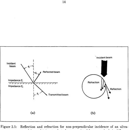
Figure 2.5: Reflection and refraction for non-perpendicular incidence of

an ultrasound beam . . . . .

Figure 2.6: Scattering of sound at small interfaces

Figure 2.7: Block diagram of simplified pulse-echo instrument

Figure 2.8: The sequence of signal conditioning steps often implemented 14

16

18

in processing of the received ultrasonic echoes. . . 20

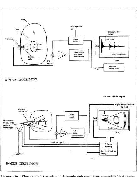
Figure 2.9: Elements of A-mode and B-mode pulse-echo instruments 22

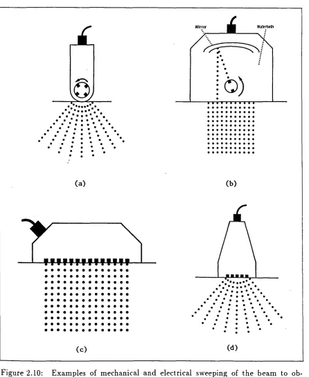
Figure 2.10: Examples of mechanical and electrical sweeping of the beam

to obtain B-mode images . . . . . 24

Vlll

Figure 3.2: Approaches to obtain the reference and attenuated spectra for

log-spectral difference technique of attenuation estimation .. 37

Figure 3.3: Illustration of shift of the spectrum to lower frequencies as an

ultrasonic pulse propagates through an attenuating medium 39

Figure 3.4: Principle of gating at a depth and measuring the signal

am-plitudes across the defined plane for so called C-mode analysis 44

Figure 3.5: Typical graph showing decrease of zero crossings density along

the depth of the tissue mimicking phantom . . . 46

Figure 4.1: System set up for ultrasonic scanning of tissue samples 49

Figure 4.2: Left side view and top view of ultrasonic scanning tank .51

Figure 4.3: Impulse responses and power spectra of the ultrasonic

trans-ducers used in this study . . . .. 54

Figure 4.4: Relative fat/muscle contents and distribution for tissue

sam-ples used for attenuation measurements .56

Figure 4.5: Schematic of data acquisition system .57

Figure 4.6: Computer Oscilloscope screen, displaying the digitized signal

Figure 4.7:

Figure 4.8:

Figure 4.9:

and controls . . . 58

Typical waveforms at various stages of data acquisition

Flow-chart of data acquisition software . . . .

Flow-chart of data analysis for attenuation calculations

61

64

66

Figure .5.1: Echoes from two sides of the Plexiglas cylinder . . . . . 73

Figure 5.3: Plot of tissue thickness vs. attenuation, showing increase in

1

CHAPTER

1.

INTRODUCTION

Ultrasound applications to the fields of medicine, agriculture, and food are

rela-tively recent developments which parallel rapid growth in electronic and signal

pro-cessing technologies. After the piezoelectric effect (upon which the generation and

detection of an ultrasound signal depend) was noted by Pierre and Jacques Curie in

1880, it was only in early 1940s when the first use of ultrasound in medical imaging

was reported. Since then, in last 45 years, ultrasonic techniques have become an

integral part of diagnostic imaging.

Ultrasound imaging techniques non-invasively obtain information about size and

structure of the tissues, and functions of the organs of the body. The interactions of

transmitted ultrasound with tissue structures give rise to the information which can

be visually displayed. This information is therefore directly related to acoustic

prop-erties of the tissues and is essentially different from that supplied by other diagnostic

tools such as an x-ray or isotope imaging. Because of its marked superiority

(particu-larly for safety, size and cost) over x-ray for soft-tissue visualization, ultrasonography

is rapidly supplementing, and in some instances, replacing x-ray for soft-tissue

visu-alization. Many applications in obstetrics, gynecology, hepatic. breast, cardiac, renal,

pancreatic, neurological, and vascular imaging are now standard. Work is in progress

and even to find parameters for pathology differentiation.

In recent years, many ultrasonic parameters have been found to have potential for

tissue characterization. These include attenuation, velocity, reflection, and scattering.

Advanced signal processing and pattern recognition techniques are applied to extract

information about particular parameters. Attenuation has been found to have

po-tential for characterizing the tissues because tissues differ in their attenuation values

for ultrasound. These might be used to differentiate the tissues, to diagnose various

pathologies, or to improve the ultrasonic images. In the meat industry, this could be

applied to differentiate (and ultimately, to grade) samples with varying contents and

distribution of fat and muscle tissues.

The purpose of this research was to develop a personal computer based system

by which the ultrasonic attenuation parameter for different tissue samples could be

estimated, and its potential for tissue characterization/ differentiation could be

deter-mined. Specifically, this involved the following objectives:

• Set up a simple hardware system that can take several A-scans of a tissue sample at varying angles, digitize the signal at varying depths of the sample and at high MHz sampling rate, and store it in a computer.

• Find an appropriate method for estimating attenuation of ultrasound in the tissue sample from the stored signal, and develop appropriate signal processing routines.

• Analyze the attenuation results in order to determine their correlations, if any, with relative fat/muscle contents in different tissue samples.

3

Chapter 2 reviews the basics of ultrasonics and describes some parameters useful

for tissue characterization. The attenuation as a tissue characterizing parameter is

discussed, in detail, in Chapter 3. It also reviews the attenuation data for normal and

pathological tissues, and their clinical significance. Recently developed techniques for

estimating attenuation in tissues is reviewed in detail, since finding the best suitable

method for fat/muscle differentiation was the first and perhaps crucial step in this

research.

The development of the personal computer based data-acquisition system is

de-scribed in Chapter 4. It also describes the developed software, implementing the log-spectral difference method of attenuation estimation. The results of this study

are presented in and discussed in Chapter 5. The attenuation was found to be an

CHAPTER 2.

BASICS OF ULTRASONICS

8

The phenomenon of ultrasound is the same as that of normal audible sound.

It occurs when mechanical vibrations in one region of a medium are transmitted

to another region by the mechanical interaction of the atoms and molecules of the

medium. Ultrasound is the term used to describe the sound when pitch is too high

for human ears to hear. The lower limit of the ultrasonic spectrum is usually taken as

about 20 KHz. The frequency range of ultrasound for medical applications is usually

between 1 MHz and 20 MHz. rJ

Generation and Detection of Ultrasound

There are several types of devices that can be used to generate and detect

ul-trasonic waves. The most common type of transducer used in medical ultrasound

employs the piezoelectric effect (Greek word piezein means to press). This is

the property of certain materials where an application of an electric field causes a

change in physical dimensions and vice versa. Commonly used (natural and

syn-thetic) piezoelectric materials are quartz, barium titanate, lead zirconate titanate

(PZT), or poly(vinylidine fluoride) (PVDF).

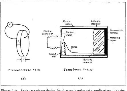
As shown in Figure 2.1a, two opposite faces of the transducer disc are plated with

.5

the thickness 1 of the transducer, whose magnitude is given by E:; = V/l (assuming

the diameter is much larger than 1).

The expansion or contraction of the transducer,~or this so called thickness mode

of orientation~ depends on the polarity of the signal. Oscillating signals cause the

transducer to vibrate, resulting in propagation of sound waves into the medium with

which the crystal is in contact. The most efficient transduction of energy occurs

at natural resonance frequency. This is determined by thickness of the piezoelectric

element; the thinner the element, the higher the frequency.

Piezoelectric -Fil.m

(a)

Plastic case

Acoustic insulator

Backing material

Transducer design

(b)

Piezoelectric element

Matching

[image:15.612.77.521.305.622.2]

layP.r:J

Figure 2.1b shows the basic design of a single-element non-focused transducer.

Such a transducer is used both as transmitter and receiver. A flat, circular disc of

piezoelectric material is mounted coaxially in a cylindrical case. The backing material

plays a major role in damping out the transducer oscillations when excited by a pulse.

Acoustic impedance of the backing material is matched to that of the piezoelectric

element to reduce reflections at the interface. Also, it is filled with special

sound-absorbing material (e.g., aluminum-filled epoxy or tungsten-filled epoxy) to damp

the oscillations, resulting in the transmission of short duration acoustic impulses

into the medium. Attachment of impedance-matching layers to the front face of the

transducer provides more efficient transmission of sound waves from the transducer

element to soft tissue and vice versa.

Frequency Characteristics of the Transducer

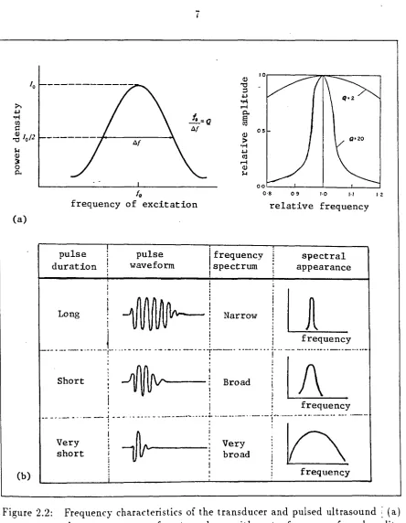
The frequency response of a transducer system is sometimes described by a term

called quality factor or Q-factor. It is defined as a ratio of resonance frequency

to bandwidth (for -3 dB power). As shown in Figure 2.2a! higher

Q

means narrow

bandwidth. The magnitude of Q is mainly determined by the losses encountered in

the transducer.

For pulse-echo system, the bandwidth depends upon the pulse duration; the

(a)

(b)

i

1·0r----"="'~=_---~

~=Q

at

at

tg 09 1·0 1·1

frequency of excitation _{relative frequency}

pulse duration

! _pulse

waveform

I

,spectrum frequency \

spectral appearance

Long

i

~

i

Narrow

i

LL

1

1

i

frequency

'---!---

---t--

---j-

rl\·

f\'.' .... ' .. _ ... .

Short

~!

Broad

LLL

frequency

.

.

.. --~ -_ .. -.- - i .. -~ -. _6 __ - ---... -- ... :- ---- .. -·-··---1~ ... · - ... - .. ----_ ... -.. -_.-Very

short

.

.

"

.

Very broad

frequency

1·2

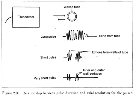
[image:17.612.77.521.67.639.2]

Axial Resolution

The transducer frequency characteristics are closely related to the axial resolution

of pulse-echo system. Axial resolution is limited by the pulse duration; the shorter

the pulse duration. the better is the axial resolution (Figure 2.3).

Transducer

Long pulse

Short pulse

Very short pulse

Walled tube

I

~O

\..--- Echo from tube

~n~ Echoes from walls of tube

-'~U~~r--Inner and outer

~es

Figure 2.3: Relationship between pulse duration and axial resolution for the pulsed ultrasound (the shorter the pulse duration. the better the axial resolu-tion)

Beam Pattern and Lateral Resolution

The sound beam produced by an unfocused circular transducer maintains the

[image:18.612.71.515.216.534.2]

9

as near field or Fresnel zone. At larger distances, the natural divergence begins to

spread the transverse extent of the beam, referred to as far field or Fraunhofer zone

(Figure 2.4).

t

(a) 2a

-1,-,-r---+-__

L

l·OI-r-;.--k--+--~';""oo;;;;::----1r----t---+---I

(b) ~ 0·5

HtHH--t-r--J'----i'---t--.=o..;o;:::::---t--...

O~~-~---~--~---~---~--~

0·0 (i)

Axial distance (> • .1 aZ)

(c)

"0" '.' ,: ".,,-. \

@

"-···'···8:---0····

..

·-:",., __ , . ) .:"',, ", ['0." (,,)

.:.~

( i ) (ii) (iii) (iv) (v) (vi)

Figure 2.4: The ultrasonic field of a plane disc transducer [ (a) conventional textbook representation of the field, (b) relative intensity distribution along the central axis of the beam. and (c) ring diagrams showing the energy distribution of the beam sections at positions indicated in (b) 1

The lateral resolution for pulse-echo system is most closely related to the

transducer beam width at the depth of interest. The beam width from an unfocused

transducer is generally too wide to give adequate lateral resolution. Therefore, a lens

or other focussing scheme (such as a spherical reflector or focused annular array of

small spot at the focal plane. The size (i.e., lateral dimensions) and the depth (i.e.,

axial distance over which the beam maintains its approximate focused size) of focus

are important parameters determining lateral resolution. Recently the approach has

been to generate a moving focus for transmitter and receiver, using complex electronic

circuits, for maximum possible resolution.

Transducer Selection

We have seen that the transducers vary in frequency characteristics, focal zone,

and face diameter. Choosing the correct transducer for a specific scanning situation

is essential. The selection of the center frequency of the transducer is a trade off

between the penetration depth of ultrasonic beam and axial resolution. Visualizing

deep structures requires more penetration; therefore, a lower frequency transducer is

desired which, in turn, gives less axial resolution. As a general rule, it is best to use

the highest frequency that allows adequate penetration.

The focal zone of the transducer is the distance range at which the lateral

res-olution is best. It is selected according to the depth of the structure to be scanned.

The diameter of the transducer face is an important factor when the window, through

which the transducer scans the structure, is small; e.g., intercostal spaces. In such

sit-uations, it may not be possible to achieve proper focal zone. For abdominal scanning,

an array of transducers is widely used.

Thus, the transducer selection is a matter of compromise: frequency vs.

pene-tration, and focal zone vs. face size. It may be helpful to examine the same area with

11

Ultrasound/Tissue Interactions

When an ultrasonic pulse travels through the tissues of the body, it undergoes

continuous modifications, which depend on characteristics of sound waves as well

as tissues. This section describes some important parameters of ultrasound/tissue

interactions.

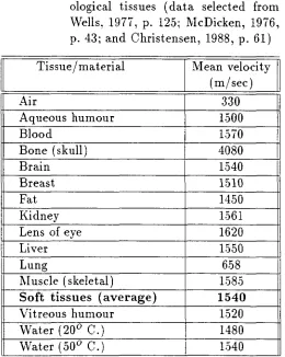
Velocity

The speed at which ultrasound travels through a medium depends on the density

and compressibility of the material. The more solid the material, the greater is the

velocity of sound. Table 2.1 shows the values for biological tissues.

As seen from values for water at different temperatures, the velocity increases

with the temperature. It also depends on condition of the tissue, e.g., dead or living.

In ultrasonics for tissue characterization, there are a few situations, listed below, in

which the knowledge of the velocity is relevant.

1. For conversion of pulse-return time into the depth of tissue.

2. To calculate the acoustic impedance of tissue, which allows echo SIze to be estimated.

3. Refraction (deviation of ultrasonic beam) occurs at tissue interfaces when ve-locity differs in two tissues.

Table 2.1: Mean velocity values for selected bi-ological tissues (data selected from Wells, 1977, p. 125; McDicken, 1976, p. 43; and Christensen, 1988, p. 61) Tissue / material Mean velocity

(m/sec)

Air 330

Aqueous humour 1500

Blood 1570

Bone (skull) 4080

Brain 1.540

Breast 1510

Fat 1450

Kidney 1.561

Lens of eye 1620

Liver 1550

Lung 6.58

Muscle (skeletal) 1.58.5

Soft tissues (average) 1540

Vitreous humour 1.520

Water (200 _{C.) 1480}

\Nater (500 _{C.) 1.540}

Acoustic Impedance and Reflection

Acoustic impedance of tissue is the resistance exerted by tissue to the sound propagation; it is given by the product of tissue density (p) and the velocity of sound

[image:22.612.166.426.136.462.2]

13

Specular reflector is the term used for a large, flat surface reflecting a perpen-dicularly (or normally) incident beam. Here, the reflected beam is also perpendicular

to the surface, so the same transducer can receive it. Specular reflection is very

com-mon in abdominal scanning; examples are capsules of the liver and kidney, the gall

bladder, and the aorta.

The size of echo due to reflection at a particular interface is expressed as the

ratio of reflected wave amplitude to the incident wave amplitude. This ratio is also

known as reflection coefficient (R).

where

R _ _ Pr _ _ Z.=....1 _-_Z-=:!.2

- Pi - Z1

+

Z2

pressure amplitudes of the incident and the reflected beams,

impedances of the tissues making the interface.

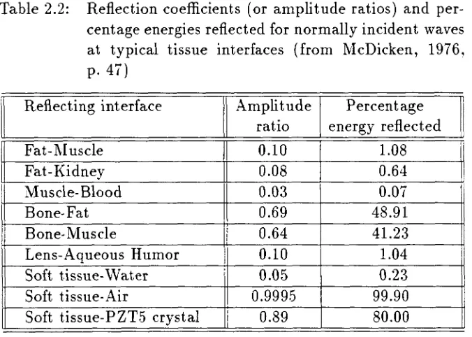
Amplitude ratios for boundaries of interest are shown in Table 2.2. The values

from the table explain why scanning through lung or gas in the bowel, or through

bone is difficult, and also why water is used as a coupling medium.

Refraction

For non-perpendicular sound beam incidence, the beam bends at the interface

if the speed of sound changes across the interface; this causes the transmitted beam

to emerge in a direction different from the incident beam. This is refraction and is

Incident beam

Z

Reflected beam I fJr

'~~;n;e,z."" ~'"

_{Impedance Z. I}

~

e,

r .. n,mltted bo.m

(a)

Incident beam

(b)

[image:24.612.74.517.76.517.2]

[image:25.612.127.465.127.368.2]

15

Table 2.2: Reflection coefficients (or amplitude ratios) and per-centage energies reflected for normally incident waves at typical tissue interfaces (from McDicken, 1976, p.47)

Reflecting interface Amplitude Percentage ratio energy reflected Fat-l\Iuscle

II

0.10 1.08

Fat-Kidney

_.

0.08 0.64

M uscle- Blood 0.03 0.07

Bone-Fat 0.69 48.91

Bone-Muscle 0.64 41.23

Lens-Aqueous Humor 0.10 1.04

Soft tissue- \Vater 0.05 0.23

Soft tissue-Air 0.9995 99.90

Soft tissue-PZT5 crystal 0.89 80.00

Scattering

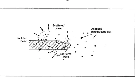
For smaller dimensions (about the magnitudes of wavelength of incident ultra-sonic pulse) of interfacing surface, the incident wave is reflected in all directions and is said to be scattered (Figure 2.6). When the dimensions of scattering objects are very much less than the wavelength, it is known as Rayleigh scattering. Since the scattered wave spread in all directions, echo signals detected from a volume containing small scatterers are not highly dependent on the orientation of individual scatterers. This is in contrast to the strong orientation dependence seen for specular reflectors.

Incident

Scattered wave

o o

Acoustic

o o 0 inhomogeneities

o

0--- /

beam ~77~7z~7077~~~~ o

o

o

o 0

~,' 0

,t... Scattered

,. -s- wave 0

o

o o

o

Figure 2.6: Scattering of sound at small interfaces (Hagen-Ansert, 1983. p. 8)

ultrasonic frequencies.

Backscatter coefficient is the term used to describe the ratio of energy

scat-tered back through 180 degrees to incident energy, per unit area. Examples of small

scatterers are red blood cells and multiple air-filled alveoli of lung tissue (where the

scattering is so severe that 1 MHz ultrasound wave is considered non-penetrating to

lung regions).

Absorption

Absorption of ultrasound is the process by which a portion of originally organized

acoustic energy is transferred to subsequent heat. (F nder ordinary circumstances

with diagnostic ultrasound. the amount of heat produced is too small to cause a

[image:26.612.78.516.85.341.2]

17

frequency of sound; therefore it is said to exhibit dispersion.

Absorption and its mechanisms are rarely considered in isolation in routine

clin-ical techniques. Total attenuation, which includes a number of other factors as well,

is a more relevant quantity.

Attenuation

As a sound beam traverses through a medium, its amplitude and intensity are

reduced as an exponential function of distance; this is referred to as attenuation. It is

the result of interactions between ultrasound and tissue including absorption,

reflec-tion, and scattering. Mathematically, attenuation is defined in terms of attenuation

coefficient (a), in the expressions

where 1

Ao

n

A = Ao e- a1

acoustic path length in attenuating medium amplitude at I = 0

power of frequency dependence of a

ao a constant.

As seen from these equations, attenuation increases with increasing frequency,

which limits the maximum frequency that can be used to scan the particular depth of

tissue or region of body; the working frequency range is typically 1-5 MHz for scanning

the abdomen, heart, or head, and .5-20 MHz for eyes. Thus, by limiting the maximum frequency, attenuation also limits the range resolution indirectly. Since attenuation

TIMER

PULSER t-- , . RECEIVER

-TRANSDUCER

-r - - - -, r - - -,

I I

I ITISSUEI I

I I I I

L _ _ .J

L _ _ _ .J

[image:28.612.76.512.142.377.2]

DISPLAY

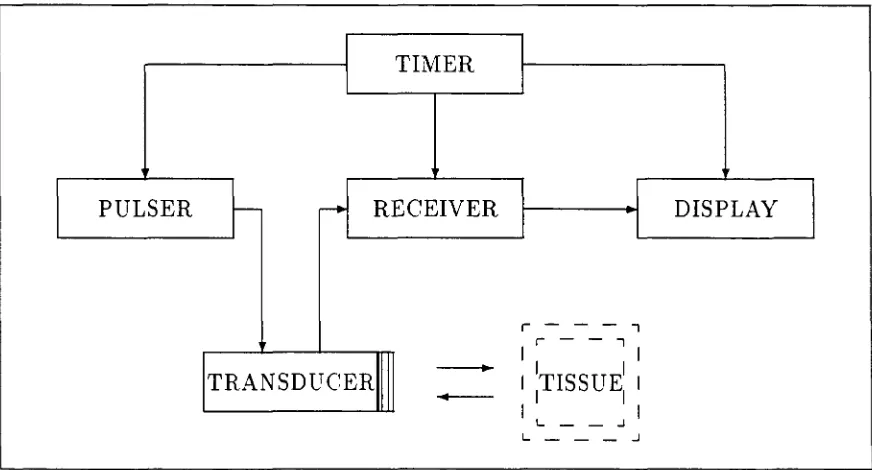
Figure 2.7: Block diagram of simplified pulse-echo instrument

Ultrasonic Instrumentation

Pulse echo ultrasound is widely used to localize and image structures in the body. The basic principle is that the distance between transmitter and reflector,

d,

is

c/2t

where c is average speed of sound in the tissue and t is delay between transmitted pulse and received echo. The simplified block diagram of pulse echo instrument is shown in Figure 2.7.

Pulser

19

bandwidth of the transducer as mentioned earlier. The acoustic power is determined

by amplitude of the pulser output.

Receiver

The receiver detects and amplifies the echoes. If only one transducer is used, the

fraction of time that the transducer is actually emitting or receiving is indicated by

duty factor, which is the dimensionless product of the prf (pulses/sec) and the time

duration of each pulse (sec/pulse). Sound beam attenuation in tissue is compensated

by using swept gain (also called TGC for time gain compensation) in the receiver.

Signal Processing

Besides amplification, the echo signals are often processed by rectification,

com-pression and rejection to condition them for effective display. These basic steps are

illustrated in Figure 2.8.

Display

A-mode is a one-dimensional display of echo amplitude, as shown in Figure 2.9a.

This was widely used to diagnose midline shifting of brain (due to edema, hematoma,

etc.) by comparing the distance of midline of brain (i.e., echo from Fax cebrii) from

Figure 2.8: The sequence of signal conditioning steps often implemented in processing of the received ultrasonic echoes

(Modified from Christensen, 1988, p. 134)

(a) unprocessed, amplified echoes;

(b) after demodulation (rectification and smoothing), yielding the pulse envelop;

(c) time gain control (TGC) amplification; (d) logarithmic compression;

(e) elimination of signals below threshold setting; (f) sweeped B-scope; and

UNPROCESSED SIGNAL

(a)

(b)

/1\

AFTER DEMODULATION

1\

(c)

/f\

AFTER TIME GAIN CONTROL

.0,

}LA

(d)

AFTER NOISE REDUCTION

(e)

1\1\

(f)

SWEEPED B-SCOPE

~---

....

~--

- -

--~-

-..----

-.----TRIGGERED B-SCOPE

-_._--A-MODE INSTRUMENT

Movable

Mechanical

linkage with _---;"=-_'1\1' .. ~ ...

position transducen

B-MODE

INSTRUMENT

T/R

5witch

Position signals

22

Pulse repetition nte

Time variable cain. "iCnal condilioninl

TGC

signal

conditioning

Cathode ny tube display

tAmPlitude

d

Cathode ray tube display

o aeam

stcerin&

Sawtooth voltage

.... ----+1 sweep

'---_ _ _ ---J

[image:33.612.86.524.85.653.2]

B-mode is two dimensional display where the echo amplitude is modulated

into brightness of the displayed beam (also called gray scale or z-axis modulation).

This is shown in Figure 2.9b. The image is constructed from several A-mode signals

taken at different angles. Most commercially available ultrasonic imaging systems use

a variety of scanning methods. These include mechanical (rotating, oscillating, etc.)

and electronic (linear array, phased array and annular array) scanners. Some examples

are illustrated in Figure 2.10. The advantages of these complex arrangements are real

time (therefore, also called real time scanner), precision scanning of larger area of

tissues with better axial, and in case of annular array, lateral resolution.

C-mode refers to through-transmission imaging in which the ultrasound pulse

IS transmitted from one side of the body through to receiving transducers on the

opposite side. Attenuation and velocity data may be obtained by this method.

Ultrasound Applications for Tissue Characterization

Ever since the use of ultrasound for tissue characterization began, it has grown

tremendously, almost as a separate discipline. It is the second most widely used

imag-ing technique, beimag-ing next only to radiology. Ultrasonic tissue characterization involves

the determination of propagation characteristics (velocity, attenuation, backscatter,

etc.) of ultrasonic energy in various tissues. In the medical field, tissue

charac-terization applications range from detecting a fetus in the uterus to differentiating

pathologies of liver, breast·, eye, etc., which can not be easily diagnosed by other

methods.

[image:35.612.83.529.97.640.2]

• • Figure 2.10:

.

• •

.

-

...

:::

...

•• •• • • • • ••• •• •

•

••••• •

•

• • • • •• • • • •• •• • • •• • •• • • • • • •

:

: :

.. ..

.

• _• • • • •

•

• (a)

•

•

• • •

•

•

•

•

•

•

•

• •

•

•

•

• •

•

• •

•

•

• •

•

•

•

• • •

•

• • • •

• •

•

•

•

• • • •

•

•

•

•

•

•

•

•

•

•

• • • • •

•

• • • •

•

•

•

•

• • • • • • • •

• •

• •

•

•

• • • •

•

•

•

•

• • •

•

•

•

•

•••••••••••••

•

•••••••••••••

• •••••••••••••

• •••••••••••••

(c) 24 ••

•

•

.

• •

•

_• •

b)

•

• • • •

•

••••••••••

•

•••••••••• • ••••••••••

·

_{• ••••••••••}

... .

• •••••••••• • ••••••••••

·

_·

... .

_{... .}

• ••••••••••

•

•••••••••• (b)

-

... .

.

...

-

... .

..

...

..

• • • • • • • • •

...

:

... .

• • • • • • • • •

.

•

.

•

•

• • • • • • • • • (d) • • •

.

• •

.

_• • • • _• • • •

26

CHAPTER 3.

ULTRASONIC ATTENUATION:

BACKGROUND

AND LITERATURE REVIEW

As defined in the previous chapter, attenuation, in simple terms, is defined as

a loss in acoustic intensity (power per unit cross-sectional area) as a transmitted

ul-trasound wave passes through tissue or any other medium. This chapter describes

the attenuation phenomena. The data for biological tissues are given and clinical

significance of some primary encouraging results are discussed. It also reviews

var-ious methods of estimating attenuation in clinical situations and their potentials in

characterization of fat and muscle tissues.

Mechanisms for Attenuation

Attenuation is caused by number of processes such as absorption, scattering,

reflection, refraction and wavefront divergence.

In

addition, when an ultrasound beam

exits from tissue, additional losses may be detected that depend on the characteristics

of the measurement apparatus, such as transducer aperture. For example, portions of

the incident beam may be refracted or scattered and may never reach the measurement

transducer.

A bsorption is the fundamental tissue parameter responsi bIe for attenuation

at-tenuation. Reflection, scattering and absorption contribute the most for measured

attenuation.

Units of Measured Attenuation

By definition, attenuation can be expressed in units of intensity (watts/ cm2 ) or

power (watts) lost per unit distance. Unfortunately, it is fairly difficult to interpret

and calibrate instruments absolutely, since power levels are very low and vary with

transducer selection. It is customary, therefore, to calibrate output levels by

com-paring them with a fixed arbitrary level using the decibel (dB) notation. Usually

the output power is compared to input power for measuring attenuation of whole

tissue; or recently the approach has been to compare powers at varying tissue depths

for statistically better estimates of attenuation, particularly for inhomogeneous

tis-sues. Attenuation can also be expressed as a ratio of wave echo amplitudes (pressure

amplitude in voltage) in decibel notation 1. Thus,

where

Power attenuation

Amplitude attenuation

10

10glO(~)

dB

20 log 10

(4;;)

dB

reference and new power levels reference and new amplitude levels.

The replacement of factor of 10 by 20 in amplitude attenuation is related to the fact that on conversion from power to voltage, the voltage (V) appears as a square (V2)

28

and 10 log10 V 2 = 20 loglO V.

When a wave is attenuated in a medium, the power levels and amplitude levels

decrease at the same rate if they are measured in dB with respect to the reference level.

It is therefore common practice to talk of attenuation in terms of dB per centimeter

depth of tissue, without specifying whether power or amplitude is being discussed.

Also, when measured thus, it is found to increase linearly with frequency, for most soft

tissues; so it is expressed per unit frequency (i.e., per MHz) or at specific frequency

(e.g., center frequency of transducer). Thus, the units of measured attenuation (i.e.,

a or aU) as defined in Chapter 2) are:

I

Units of Q :

I

I

or dBcm- 1 at 2 .. 5

I MHz

I

Since it is difficult to assess the individual contribution of mechanisms in routine

diagnostic techniques, it is quite preferable to estimate the more relevant quantity,

attenuation as a whole or total attenuation. In some literature, attenuation is

referred to for only a single mechanism (e.g., absorption); it is recommended that

these misleading terms should be avoided and the general term attenuation should be

reserved for total attenuation.

Frequency Dependence of Attenuation

The importance of the various mechanisms is dependent on the wave frequency;

therefore, the total attenuation is also a function of frequency. The attenuation of

soft tissues increases monotonically with frequency in low MHz range. This frequency

(Lele et al., 197.5; Narayana and Ophir, 1983a). The frequency derivative or slope

of this monotonically increasing function of frequency provides an useful index of

attenuation. It has been shown that this slope is quite independent of whether or not

the tissue attenuation exhibits a linear dependence on frequency (Jones and Behrens,

1981; Narayana and Ophir, 1983b).

Many investigators have worked to determine frequency dependence of

attenua-tion for various normal and pathologic tissues. In general, for most soft tissues, this

dependence is linear or almost linear (i .e., power of frequency dependence around 1)

for most practical purposes. Non-linear frequency dependence has been found for

blood, bone and lung tissues.

Attenuation Data for Biological Tissues

Biological tissues can be characterized ultrasonically by their attenuation,

ab-sorption, and velocity, which correlate well with the presence of major tissue

compo-nents of water and protein, particularly collagen (Johnston et al., 19(9). Compiled

data of average attenuation for tissues by categories are shown in Table 3.1. As seen

from the table, the structural tissues such as tendons and bones tend to be more

attenuating than visceral organs such as liver, brain and kidney. Also, note that the

frequency dependence of attenuation for blood, bone and lung is not linear, while

most soft tissues exhibit a linear dependence. Increasing attenuation also correlates

to decreasing water content, increasing protein content and increasing speed of sound

30

Table 3.1: Average attenuation for biological tissues by categories (data selected from Johnston et al., 1979; Dunn, 1975; and Goss et al., 1978 and 1980)

Tissue Attenuation , General trends

il

attenuation at f=1MHz Tissue Remarka water collagen sound

I'

categories (dB cm- 1 ) content content velocity I

Very low 0.026 serum

-

_T

increa.sing increa.sing

0.087 , blood , , _I f 1."20 structura.l velocity

Low 0.61 fat I

@ 37°C. protein of sound

Medium 0.87 brain

-

conten'

0.96 liver I

-0.7-1.4 _I muscleb

!

-I

1.9 breast I

-i

I

2.0 heart ,

I

II

i

-2.6 kidney , _i

-

_;1

High 4.3 tendon

_I

-

increasing

\1 Very high

>

8.7 bone

\

f l . l _{H 2 O} 1

- !

>

34 lung

I

fU'o

₁

i

Ii

- I cont~nt .~

a fn represents the power of frequency dependence for attenuation in the power law model aU) = aofn (spaces indicate a linear dependence, i.e., f1).

bStriated muscle; attenuation along the fibers is higher than that across the fibers.

Half-value Layer Thickness: To give some appreciation of the role of atten-uation in practice, the thicknesses of tissues required to reduce ultrasonic intensity by half (-3 dB) are listed in Table 3.2. Some interesting points can be noted from the table and related to practicabilities of imaging tissue structures.

1. Firstly, many soft tissues have similar attenuation characteristics, e.g., for brain and liver, the intensity of 2 MHz ultrasound is reduced by half in about 2 cm. Blood, on the other hand, is less attenuating and this helps the visualization of cardiac structures.

[image:41.612.85.522.150.397.2]

Table 3.2: Thicknesses of biological tissues required to attenuate intensity of an ultrasound beam by half (-3 dB) (McDicken, 1976, p. 58)

Tissue / material Thickness (in cm.) of tissue at

1 MHz 2 MHz 5 MHz 10 MHz 20 MHz

Aqueous humour

-

-

6 3 1.5

Air 0.25 0.06 0.01

-

-Blood 17 8.5 3 2 1

Bone 0.2 0.1 0.04 -

-Brain 3.5 2 1

-

-Caster oil 3 0.7.5 0.12

-

-Fat 5 2.5 1 0.5 0.25

Kidney 3 1.5 0.5

-

-I Lens of eye

-

-

0.3 0.15 0.07

Liver 3 1.5 0.5

-

-I Muscle 1..5 0.7.5 0.3 0.15

-Perspex 1.5 0.7 0.3 0.1.5 0.07

Polythene 0.6 0.3 0.12 0.6 0.03

I Soft tissues (average) 3 1..5 0.5 0.3 0.1.5

i Vitreous humour

I

6 3 1.5

-

-II

Water

II

1360

I

340

I

54

I

14 3.4

to the uterus. \Vater itself is very useful because of it.s extremely low absorption; for most practical purposes, water can be regarded as lossless and can therefore be used in immersion scanning with no loss of sensitivity.

3. Muscle is of special note in that it is anisotropic and a difference of a factor of 2 .. 5 exists between the attenuation across and along its fibers.

4. The high attenuation in the bone, about 20 times that of soft tissues, creates many problems for ultrasonic scanning. B-scanning of the head is primarily difficult; bones also limit viewing access to the heart, eye and abdomen .

. 5. Gas bubbles in lung cause high attenuation by extremely strong scattering and absorption of t.he ultrasound and this makes it almost impossible to penetrate a normal lung with diagnostic ultrasound. Lung also limits examination of heart and much of the thorax.

[image:42.612.105.506.150.439.2]

32

it is a convenient medium for constructing test and training phantoms.

7. Absorption in air is very high at diagnostic frequencies. Because of this and low acoustic impedance, transmission of ultrasound in air ceases to be practical above 0 .. 5 MHz (McDicken, 1976, p. 59).

Clinical Significance of Attenuation

Tissue attenuation has been measured in vitro and in vivo by many investigators

and some initial clinical results for several different estimation techniques have been

obtained, particularly for liver, breeast, eye, and uterus.

Some encouraging consistency has been noted among the results obtained using

several different methods of estimation. Attenuation has been found to have

poten-tial to become a clinically measurable parameter for differenpoten-tial diagnosis of certain

pathologies. Attenuation measurements in vivo and their correlation with biopsy and

autopsy results has enabled separation of normal from pathologic tissues. Most

in-vestigators have chosen the liver as the target organ, primarily because of its large

size, homogeneous nature of the backscatter, the ease of access and confirmation of

the results through easy liver biopsy. Table 3.3 shows the attenuation data for liver

pathology differentiation.

It should be noted that the ultrasonic attenuation may not serve as the only

pa-rameter for differential diagnosis, but it surely has potential to become an important,

Table 3.3: Summary of in vivo measurements of ultrasonic attenuation in liver using a variety of methods (Jones, 1984)

II

Patholog~

Normal

I

Cirrhosis

II

Hepatitis

I

Fatty

Attenuation

• magnitude: 0.5 dB/cm @ 1 MHz (range 0.4 - O.i)

• frequency dependencea : 1.05 (range 0.95 - 1.15) • 50% - 60% higher than corresponding normal • slightly greater frequency dependence

• 30% - 40% lower than corresponding normal • high (when scattering dominates), or

low (when absorption dominates)

• higher frequency dependence (range 1.0 - 1.4)

aRepresents the power, n, in the power law model a(f) = Ctofn.

Methods of Attenuation Estimation

II

I

J

l.Tltrasonic attenuation has been measured in vitro by many investigators ever

since the field of diagnostic ultrasound began. In last fifteen years, there has been

good progress in this area and many in vivo methods, too, have been developed

to estimate attenuation in a clinically useful manner. The goal in measurement of

attenuation is to provide an objective and reliable index to quantitate the subjective,

equipment-dependent estimates of attenuation that clinicians have found useful in

interpreting ultrasonic images. Some uses for measurements of attenuation include:

• Improved time gain compensation for imaging (Melton and Skorton, 1981).

• Compensating backscatter measurements for the attenuation of intervening tis-sue (Cohen et al., 1982; and O'Donnell, 1983).

• Estimating local values of attenuation for purposes of tissue characterization (Shawker, 1984; Maklad. 1984; and Jones, 1984).

• As a long term goal, quantitate the backscatter and attenuation imaging

34

Qualitative estimation in B-mode On the standard B-mode image, the effects of

attenuation are subjectively observed by ultrasonographer. Attenuation of localized

lesions is judged by the appearance of the posterior echoes, i.e., amplitude of the

returning echoes from the far side of a lesion. Terms such as acoustic enhancement

(echo amplitude higher than the surrounding tissues) and acoustic shadowing (total

absence of the posterior echoes) are qualitative descriptions of this posterior echo

amplitude. This helps distinguish cystic and solid masses.

Attenuation in large masses or entire organs is generally estimated by the relative

difficulty of beam penetration. This is subjectively evaluated by noting the

transdu-cer frequency, the instrument gain, and the time-gain-compensation (TCG) settings

required to penetrate an organ or large mass, and to uniformly display the echoes in

near and far fields of the transducer.

Quantitative estimation in reflection Over the past several years, several pulse

echo techniques for quantitative estimation of attenuation have been developed, and

some initial clinical results have been obtained, particularly for the liver. These

methods can be grouped in time domain and frequency domain methods. In general,

time domain methods are adaptable to real time implementations, which feature speed

at the expense of flexibility. On the other hand, the frequency domain techniques

allow flexibility of implementation, but tend to require off-line processing.

An excellent review of these techniques could be found in literature (Miller, 1984;

and Flax, 1984). Since the part of this research was to select the best method for

application to fat and muscle characterization, some methods are discussed in detail

Frequency Domain Methods

These methods fall generally into two main kinds: spectral difference methods

and spectral shift methods. A relatively new approach of matched filter pulse

com-pression is also considered in this category.

1. Log Spectral Difference Techniques: In these techniques, the log-power

of the signal, attenuated by its path through the tissue, is compared with reference

log-power. As shown in Figure 3.1, the log-power difference is plotted against frequency

and least square slope over the transducer bandwidth is calculated. Dividing this

slope by the distance the signal traveled (in cm.), gives the coefficient of attenuation

in dB cm- 1 MHz-1. There are several approaches to obtain attenuated and

refer-ence spectra, as illustrated in Figure 3.2 and described below.

TRANSMISSION ApPROACH: Here, a broad band pulse passes through the tissue

of interest and is received by a second transducer (Figure 3.2a). The attenuation

is estimated by comparing the response obtained with only water (or physiological

saline) between transducers and the response obtained when tissue is substituted.

SHADOWED REFLECTOR ApPROACH: This represents a slight modification of

the transmission method, in which single transducer emits and receives a pulse that

passes through the tissue a second time after being reflected from a flat metal or glass

plate (Figure 3.2b).

BACKSCATTER ApPROACH: A conceptually simple approach for estimating

attenuation from backscatter signal is to compare spectra of echoes obtained from

E

1-1 oI-l () Q) P. til 1-1

~ _o

p. 00 o ...t shallow (reference) deep (attenuated) frequency (a) 36

slope of line 0:0

=

2 (shallow - deep)

frequency

(b)

Figure" 3.1: Log-spectral difference technique for estimation of attenuation [ (a) ref-erence and attenuated log-power spectra, and (b) log-spectral diffref-erence and least square fit to calculate the slope and coefficient of attenuation]

of the irregular shapes of the surface of organs of interest and the specular echoes

that a"rise from tissue interfaces are highly dependent on geometrical factors that can

not be controlled.

It is difficult to adapt the techniques just described to in vivo situations, due to

the factors listed below (Ophir et al.. 1984).

1. Tissue does not contain reliable reference reflectors, and therefore estimates must be made from a noisy statistical ensembles of scatterers. This limits the precision and spatial resolution obtainable in the estimate.

2. Evidence indicates that the main contribution to attenuation is from absorption and not from scattering. The attenuation estimates, however, rely heavily on the properties of the scatterers, such that small changes in these properties could readily result in erroneously large changes in the attenuation estimates.

(a)

reflector

transmitter

~

& receiver

--1

114·

(b)

transmitter

& receiver ~

--4

II ••

~

shallow deep

(c)

Log-power spectra (reference and attenuated)

without

I'

~

withtissue

( \issue

without

( ~ tissue

' / "with

. tissue

shallow segment

~deep

segment

[image:48.612.84.527.113.611.2]

38

4. Various techniques estimate different quantities which are related to attenua-tion under certain assumpattenua-tions (e.g., tissue model of scatterers and specular reflection). The validity of these assumptions is difficult to ascertain.

5. Transmission and shaded reflector methods can not be adapted clinically for obvious reasons.

Consequently, most of the techniques proposed for estimating attenuation in

reflection concentrate on relatively weak backscattered signals emanating from the

interior of the tissue. Figure 3.2c illustrates steps in this method. A shallow and a

deep segment are extracted from rf A-mode signal and power spectra are obtained

using appropriate method. One common approach is to take the Fourier transform

using the Hanning window.

Assuming that the backscatter coefficient is the same in shallow and deep

seg-ments, log spectral difference can be obtained and attenuation coefficient (0:) and slope (Qo) can be calculated as described earlier. The following points should be

noted about this method.

• The mean slope exhibited by tissue volume is obtained by averaging axially (along A-mode signal) and laterally (adjacent A-mode signals). This reduces the variance (Fink et al., 1983; Lizzi and Laviola, 1976; and Kuc and Taylor, 1982).

• The optimal separation between shallow and deep pairs in rf A-mode data for axial averaging is suggested to be 2/3 of total length of the A-mode signal (Kuc et al., 1977; and Kuc and Schwartz, 1979).

• Smoothing the spectra (in frequency, autocorrelation, or cepstral domain) has some effect in improving the estimates (Robinson, 1979; and Fraser et al., 1979).

2. Spectral Shift Technique: This approach is based on the fact that soft

tissues exhibit transfer characteristics of a low-pass filter (because the ultrasonic

high frequency results in a decrease, with distance travelled, in the peak frequency,

the average frequency (centroid), and the bandwidth of the received signal in general.

This is illustrated in Figure 3.3.

[image:50.612.64.534.181.428.2]

( a)

... \f

p

o

..

_e r

s

p e c

t r

u

m

Frequency

Figure 3.3: Illustration of the shift of the spectrum to lower frequencies as an ultra-sonic pulse propagates through an attenuating medium

In these methods. models for the transmitted pulse shape and for the frequency

dependence of attenuation are assumed to relate measured changes in the spectrum

to the attenuation. Usually, the spectrum is modelled as a Gaussian with variance 0'2;

then. the shape of the spectrum remains unchanged and the variance is preserved.

The shift in frequency

(.6.f)

is proportional to the slope of attenuation (ao), the

distance travelled (I) and the variance of the pulse as

'J

fe

=

fo - aolO'~ or (3.1 )

40

has been shown that an estimate of the centroid provides a better measure of the

frequency shift than an estimate based on the peak frequency. The centroid «

1

> )

can be calculated as

Jh

I[E(f)[2

dl

<

1

>

=

_1--";1~

_ _

_

Jh

[E(f)[2

dl

h

where [E(f)[2 is the power spectrum of the windowed rf segment.

3. Matched Filter Pulse Compression Technique: This new concept

was developed by Meyer (1979 and 1982). The motivation for this approach is the

limitations of time gated pulse echo ultrasound. Tissue segments from which received

power spectra are computed can not be made arbitrarily short, because reducing

the time windows blurs the power spectra (a trade-off between axial resolution and

spectral resolution). Also, interference effects resulting from the overlap of signals

emanating from adjacent regions of tissue compromise estimates of attenuation.

The matched filter pulse compression method (also called as matched filter

cross-correlation method) overcomesthese drawbacks. It is capable of providing results that

are independent of overlaping echo wave-trains from adjacent tissue regions separated

in time by

2/6.1,

where

.6.1

is the system bandwidth. For example, for a bandwidth of .5 MHz, attenuation coefficient from tissue segments as small as 0.3 mm can be

determined independently. This has potential of high resolution attenuation imaging.

It is beyond scope of this document to discuss this method any further, but the

interested reader is urged to refer the original li terat ure (Meyer, 1979 and 1982).

for attenuation estimation techniques.

A parametric method of analysis is one which

requires the transmitted ultrasonic pulse to be of convenient mathematical

param-eters, e.g., as a Gaussian shape pulse. In contrast, a non-parametric method does

not require such characteristics of transmitting pulse. For example, frequency shift

method is a parametric one, while log-spectral and matched filter pulse compression

methods are non-parametric ones.

Time Domain Methods

Just as the attenuation information in the frequency domain is carried in the

amplitude and center frequency of the rf spectrum, so is the attenuation information

in the time domain contained in the amplitude and rate of zero-crossings of the rf

signal itself. The important advantage of time domain methods is the possibility of

real time implementation.

1. Amplitude Difference Method: In this method, the difference in the

amplitudes of backscattered echoes from two planes in the tissue is measured. This

amplitude difference is related to the attenuation coefficient o:(f).

The relationship between frequency domain and time domain attenuation is

de-scribed by simple convolutional model for backscattered signal from a pulse

propa-gating through an attenuating medium (Flax et al., 1983; and Flax, 1984). The basis

for this model is given by Eq. (3.2), assuming the Gaussian spectral shape, linear

fre-quency dependence on attenuation, negligible frefre-quency dependence of the scatterers,

where

_f

S(f)

IA(f)I~

ao

Z

fo

42

frequency

backscattered power density spectrum noise spectrum

attenuation coefficient (in dB em -1 MHz -1 ) depth of tissue traveled by ultrasound

transducer center frequency

characteristic width of transducer power spectrum.

(3.2)

Now, the total energy contained in the signal is integral over the power density

spectrum (Parseval theorem). Hence. the energy as a function attenuation and depth,

E( ao, Z), will be

E( ao, 1) = 2

10

00

S(f) df.

However, since the spectrum is Gaussian and does not change shape with attenuation,

the energy will be simply proportional to the power density at the center frequency

(fe). Thus, the energy can be described by the proportionality

E(ao,l) IX S(fe).

Using Eq. (3.2)' the backscattered energy is given as

where Ao is the Gaussian envelop amplitude at the center frequency (fe). Substituting

Eq. (3.1) for fe,

{ 2 2 2 }

Thus, the spectral energy decays exponentially, but not as a simple linear function of

ao or I, but rather with an additional quadratic term (aolo-)2. However, if the pulse

bandwidth is narrow such that 0-2 can be approximated as zero, then the quadratic

term disappears leaving the desirable relationship

( 3.4)

It is therefore possible to estimate ao by measuring the amplitudes (or

inten-sities) of the echoes from the backscattered signals from two planes separated by a

distance I. Using a method termed C-mode analysis, Ophir et al. (1982) applied

this narrowband relationship to estimate attenuation coefficient for human skeletal

muscle in vivo. In this technique, a narrowband transducer and a gating mechanism

are used to detect the narrowband signal located at a specified distance from the

transducer face. By translating the transducer back and forth over a fiat (X- Y)

re-gion, an amplitude plane will be defined at the gated depth, as shown in Figure 3.4.

The average value of all the amplitude measurements across the plane is recorded,

to reduce the effect of beam profile. Next, the transducer (or gating) is repositioned

at a different axial depth and the procedure is repeated. By simply determining the

amplitude change occurring with axial translation (l) between planes, and noting

the transducer center frequency (fa), the attenuation coefficient (ao) can be readily

determined from Eq. (3.4).

One of the main factors that affects the amplitude measurements is the axial

beam sensitivity profile. So, a knowledge of the beam profile and appropriate