Robust Scalable Visualized Clustering in Vector and non Vector
Semimetric Spaces
Geoffrey Fox
School of Informatics and Computing Indiana University
Bloomington IN 47408, USA [email protected]
Abstract
We describe an approach to data analytics on large systems using a suite of robust parallel algorithms running on both clouds and HPC systems. We apply this to cases where the data is defined in a vector space and when only pairwise distances between points are defined. We introduce improvements to known algorithms for functionality, features and performance but review state of the art as this is not broadly familiar. Visualization is valuable for steering complex analytics and we discuss it for both the non vector semimetric case and for clustering high dimension vector spaces. We exploit deterministic annealing which is heuristic but has clear general principles that can give reasonably fast robust algorithms. We apply methods to several life sciences applications.
Keywords Clustering, MDS, Dimension Reduction, Parallel Algorithms, Bioinformatics
1
Introduction
The importance of big data is well understood but so far there is no core library of “big algorithms” that tackle some of the new issues that arise. These include of course parallelism which should be scalable i.e. run at good efficiency as problem and machine are scaled up. Further one can expect that larger datasets will increase need for robust algorithms that for example when applied to the many optimization problems in big data do not easily get trapped in local minima. Section 2 describes deterministic
annealing as a generally applicable principle that makes many algorithms more robust and builds in the important multi-scale concept. In section 3, we focus on clustering with an emphasis on some of the advanced features that are typically not provided in the openly available software such as R [3]. We discuss some challenging parallelization issues for cases with heterogeneous geometries in section 4.
Further we note that the majority of datasets are in high dimension and so not easily visualizable to inspect the quality of an analysis. Thus we suggest that it is good practice to follow a data mining algorithm with some form of visualization. We suggest that the well-studied area of dimension reduction deserves more systematic use and show how one can map high dimension vector and non vector spaces into 3 dimensions for this purpose. This process is also time consuming and itself an optimization problem (find the best 3D representation of a set of points) and so needs the same considerations of parallelization. This is briefly described in section 5.
2
Deterministic Annealing
Deterministic annealing[4] is motivated by the same key concept as the more familiar simulated annealing, which is well understood from physics. We are considering optimization problems and want to follow nature’s approach that finds global minima of energy functions rather than local minima with dislocations of some sort. At high temperatures systems equilibrate easily as there is no roughness in the energy (objective) function. If one lowers the temperature on an equilibrated system, then it is a short safe path between minima at current temperature and that at a higher temperature. Thus systems which are equilibrated iteratively at gradually lowered temperature, tend to avoid local minima. The Monte Carlo approach of simulated annealing is often too slow, so we perform integrals analytically using a variety of approximations within the well-known mean field approximation in statistical physics. In the basic case, we have a Hamiltonian H(χ) which is to be minimized with respect to variables χ and we introduce the essential idea of deterministic annealing based on averaging with the Gibbs distribution at Temperature T. P(χ) = exp( - H(χ)/T) / ∫ dχ exp( - H(χ)/T) (1)
or P(χ) = exp( - H(χ)/T + F/T ) (2)
and minimize the Free Energy F combining Objective Function and Entropy,
F = < H - T S(P) > = ∫ dχ [P(χ)H + T P(χ) lnP(χ)] (3)
as a function of χ, which are (a subset of) parameters to be minimized. The temperature is lowered slowly – say by a factor 0.95 to 0.9995 at each iteration. For some cases such as vector space clustering and Mixture Models, one can do integrals of equations (1) and (2) analytically but usually that will be impossible. So we introduce a new Hamiltonian H0(ε, χ) which by choice of ε can be made similar to real Hamiltonian H(χ) but have a simpler dependence on χ such that the integrals are tractable analytically. Then we use the approximate Gibbs distribution
P0(χ) = exp( - H0(ε, χ) /T + F0/T ) (4) and calculate
F(P0) = < H - T S0(P0) >|0 = < H – H0> |0 + F0(P0) (5) where <…>|0 denotes averaging with Gibbs P0(χ) i.e. ∫ dχ P0(χ). ε is fixed in these integrals
Note that the true Free Energy satisfies the Gibb’s inequality
F(P) ≤ F(P0) (6)
which is also related to Kullback-Leibler divergence. This leads to an expectation maximization EM method with annealed variables given by the E step:
χ = <χ> |0 = ∫ dχχ P0(χ) (7)
Note there are three types of variables ε, χ, ϕ in the general case . The first variable set ε are used to approximate the real Hamiltonian H(χ, ϕ) by H0(ε, χ, ϕ); the second variable set χ are subject to annealing while one can follow the determination of χ by finding yet other parameters ϕ (the third set) optimized by traditional methods – the M step. Usually the functions have a simple dependence on ϕ allowing a trivial optimization given the values of the other two sets. Note one iterates over temperature decreasing it, but also iterate at fixed temperature until the EM step converges. The formulation above shows deterministic annealing to be generally applicable and gives a method first described by Hofmann and Buhmann for the general problem [5] as a generalization of the original theory derived by Rose, Fox and collaborators [6, 7]. The discussion here includes published [4, 8] and unpublished improvements, and the latter are noted explicitly. Further I do not think the many published ideas have ever been
integrated as efficient parallel functional libraries and that is another important contribution of this paper. Challenges in using deterministic annealing include formulating the Hamiltonians H(χ, ϕ) and H0(ε, χ, ϕ) and especially choosing the approximating parameters ε. The algebra involved in minimizing (5) can be quite difficult especially for the second derivatives needed in the splitting analysis described below in section 3.3. The resultant software complexity is at least an order of magnitude greater than simpler methods such as Kmeans which reinforces the suggestion [9] that one should build libraries that once and for all embody these most sophisticated powerful algorithms such as deterministic annealing.
3
Vector Space Clustering
3.1 Basic Central or Vector Space Clustering
Consider a clustering problem with N points labeled by x and K clusters labeled by k. In this example, the annealed variables χ are Mx(k), which is the probability that point x belongs to cluster k with
constraint.
∑k=1K Mx(k) = 1 for each x. (8)
In either central clustering (where points are in a vector space so there are identified centers Y(k)) or pairwise clustering
H0 = ∑x=1N∑k=1K Mx(k) εx(k) (9)
which is linear in Mx(k) allowing integrals in equations (5) and (7) to be done analytically.
The vector space central clustering has
εx(k) = (X(x)- Y(k))2 (10)
where points have position X(x) and cluster centers are Y(k), so:
HCentral = H0 = ∑x=1N∑k=1K Mx(k) (X(x)- Y(k))2 (11)
and one easily proves [4, 6] that the expectation E step gives:
<Mx(k)> = exp( -εx(k)/T ) / ∑k=1K exp( -εx(k)/T ) (12)
and the cluster centers Y(k) are easily determined in M step.
Y(k) = ∑x=1N < Mx(k)> X(x) / ∑x=1N < Mx(k)> (13)
We don’t discuss the non vector case here in detail except to note that equation (9) takes the same form but rather than analytic formula (10), the εi(k) are determined so that H0 in (9) approximates
HNon Vector = 0.5 ∑x=1N∑y=1N d(x, y) ∑k=1K Mx(k) My(k) / C(k) (14)
where d(x, y) is the distance between points x and y. Non vector space problems are typically specified by this pairwise distance rather than the Euclidean form of distance and scalar products.
Here C(k) = ∑x=1N Mx(k) as number of points in k’th cluster (15)
and ∑k=1K C(k) = N the total number of points (16)
3.2 Fuzzy Clustering and K-means
Looking at equation (12), we see that each point x belongs to all clusters k with a probability proportional to exp( - (X(x)- Y(k))2 /T ) which is largest for the center Y(k) that is nearest the point position X(x). At very high temperatures, the exponent is near zero and all centers have roughly equal probability – exactly equal at infinite temperature. At large temperatures, all centers coincide with a position
Y(k) = ∑x=1N X(x) / N (17)
As we anneal and the temperature decreases, the points gradually commit to a center and in the zero temperature limit, one finds a K-means solution with each point associated 100% with the nearest center; the characteristic of the K-means solution. This is an example of “fuzzy clustering” [10] which is a related technique to avoid the “early committal” of greedy solution methods that iterate hard constraints.
The idea behind annealing shown in figure 1, is that there are no false minima at high (infinite) temperature as the objective function is totally smooth there; thus we have properly minimized the free energy there. As we lower the
temperature we start at minimum solution at higher temperature and as long as we cool slowly, we are near the minima at lower temperature and not likely to get trapped; thus annealing – as seen in the physical forge – is robust as long as temperature lowered slow enough (we will discuss criteria for this below). The rough dependence of objective function on center positions can lead to false minima at finite temperature with no annealing as shown by temperatures T2 and T3 of the figure. We are approximating this process in deterministic annealing. This approximation involves replacing integrals by evaluations of functions by their mean value. This is motivated (justified) by the sharp peak in the integrands of equations (5) and (7).
3.3 Multiscale (Hierarchical) and Continuous Clustering
In many problems, decreasing temperature is a classic multiscale step with finer resolution being used as temperature T decreases. Note from equations (9) and (10) that we have factors like (X(x) - Y(k))2 / T and √T acts as a distance scale. In clustering there is just one cluster at infinite temperature (the starting point) at the mean position over all points. We already noted this above with the universal formula of equation (17) with all centers at the centroid. A critical feature of deterministic annealing is that unlike K-means, one need not feed in the “required” number of clusters. Rather one can start with just one cluster
Figure 1: The annealing mechanism for tracking true minima illustrated with 3 temperatures and two false minima at finite temperature
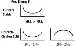
Figure 2: Stable and Unstable behavior of Free Energy F w.r.t. positions of perturbing centers
and decrease temperature from the highest value. The system becomes unstable and additional clusters “pop” out in what is a phase transition in the physics interpretation of the system [7]. This is illustrated in figure 2, showing that if one has two identical centers Y(kA) = Y(kB), at a phase transition, the system is
unstable to the combination Y(kA) - Y(kB). There are two rather different ways these phase transitions can be found. In the first method, one inserts multiple potential centers at each site and at every temperature, test stability by perturbing half in one direction and half in the opposite direction.
In the second method which my software uses, one calculates the second derivative of the free energy (the first derivative is of course zero) and tests for negative eigenvalues. This method can be quite time consuming but has advantage that it also gives a direction in which to perturb the centers. It was introduced in vector case by Rose [4] without details and our extensions for the non vector case are new. It also gives one an understanding of nature of instability. If one calculates the second derivative for the vector space clustering and transforms to the local eigendirections Y(kA) - Y(kB). and Y(kA) + Y(kB), then one find that instability corresponds to a negative eigenvalue of D by D matrix Γ given in equation (18) for the unstable combination Y(kA) - Y(kB) below where D is dimension of vector space and i and j run over vector components. The stable combination Y(kA) + Y(kB) is position of mean of two centers and the instability corresponds to their splitting apart.
Γij(k) = δij ∑x=1N < Mx(k)> - ∑x=1N (Yi(k)) - Xi(x)) (Yj(k)) – Xj(x)) < Mx(k)> / T (18)
Here one looks independently at stability of each center k. The calculation of eigendirections is
straightforward and reliable as (18) is difference of a diagonal and positive definite symmetric matrix. If one uses the power method, one need not explicitly calculate second derivative matrix but rather scalar products V.( Y(k) – X(x) ). Note as temperature T decreases, the second term in (18) gets larger in magnitude and the possibility of an overall negative eigenvalue increases. At very small T, all centers show negative eigenvalues and this can help design the annealing schedule. One aims for interesting/all centers to appear in region where (18) still
discriminates between centers. In that region, the “very elliptical” centers with unusually large |Y(k)) - X(x)| will split first and the “spherical” ones later (at lower temperature). One lowers temperature at a rate that gives enough iterations to allow all clusters to appear in this appropriate temperature regime before (18) has negative eigenvalues for all centers. As another minor benefit of explicit form of (18), note that one can estimate “infinite temperature” analytically by using simple bounds to find an “infinite” T∞ for which value (18) is guaranteed to have positive eigenvalues. It is does not matter if T∞ is an over estimate as one only has one cluster at this stage and the computation goes very fast. We use power method except for small dimension D (an
important special case) where we use analytic eigenvalue methods. Figure 3 illustrates a clustering which started with a single cluster at high temperature and finished with approximately 25,000 clusters; each new cluster being generated from a split as described above. There is structure around T=20 for reasons described in section 3.4. In deterministic annealing, one can stop in two different ways; one criterion is just reaching a particular cluster count as is essentially used in traditional Kmeans. However the results of figure 3 come from a different approach stopping the splitting at a particular value of temperature i.e. at a
Figure 3: Cluster Count versus Temperature for a D=2 LC-MS peak example[1] with 241605 points
cluster size in target space. This emphasizes the value of concept that √T is related to distance in
parameter space. In this application the cluster size is known as it corresponds to a measurement error that can be determined a priori.
There is an important technical issue that I call continuous clustering which is needed to make the above scheme work well. This was first described by Rose [4] but it is not broadly recognized and for example the important and brilliant work by Buhmann and colleagues [5, 11, 12] does not use it. Equation (12) does not directly allow a simple splitting as discussed above as if K>1, ∑k=1K exp( -εx(k)/T ) is
significantly changed if one replaces one cluster by two; i.e. the splitting affects the < Mx(k)> for all k.
One addresses this by introducing p(k) which is relative number of centers at site with position Y(k). (12) is then replaced by
<Mx(k)> = p(k) exp( -εx(k)/T ) / ∑k=1K p(k) exp( -εx(k)/T ) (19)
with ∑k=1K p(k) = 1 (20)
The probability p(k) is like Y(k), one of the parameters that are determined by analytic optimization in the M step of the free energy optimization after the <Mi(k)> are determined by annealing. One can easily
show that
p(k) = <C(k)>/N = ∑x=1N <Mx(k)>/N (21)
i.e. every center is weighted in sum ∑k=1K p(k) exp( -εx(k)/T ) by an amount proportional to their size
or equivalently that every point is equally represented in this sum – an elegant principle. Now one can implement cluster splitting at a phase transition very simply. A split cluster starts with (perturbed) positions Y(kA) and Y(kB) near original (split in direction of negative eigenvalue) and with both p(k) and <C(k)> exactly half that of original cluster as expected for splitting in two. Note (21) ensures this is consistent. Our software is the first to use this idea in both vector and non vector cases.
3.4 Trimmed Clusters with a Sponge
There are several refinements that are needed in extensions of the above formalism. One example [1, 13] involves adding a “sponge cluster” defined by
HCentral = H0 = ∑x=1N [∑k=1K Mx(k) ((X(x)- Y(k))/σ(k))2 + Mx(sponge)c2] (22)
Here we have taken a case when there is prescribed error σ(k) for each cluster as would happen if cluster spread due to an estimable measurement error discussed in figure 3. Then let’s use k=0 for the “sponge” term introduced above.
< Mx(0)> = p(0) exp( - c2/T) / (∑k=1K p(k) exp( - (X(x) - Y(k))2/(σ(k)2 T) ) + p(0)exp( - c2/T) ) (23) As T decreases we see that < Mx(0)> tends to one and < Mx(k)> to zero if k ≠ 0 if
(X(x) - Y(k))2 / σ(k)2 > c2 for all k (24) i.e. the k = 0 sponge picks up all points that have squared distance greater than σ(k)2 c2 and correspondingly all points inside “real” clusters are within this radius. The sponge seen later in figure 5(b), picks up all “stray” points not near enough to a cluster center and all clusters are cut off and the centers are calculated from equation (13) as trimmed means. This approach gives a set of well-defined compact clusters with a “dust” of stray points picked up by the sponge. In our implementation we only added sponge below the high temperatures and then annealed the constant c starting at high values and letting it reach target value at a temperature where clustering was determined apart from final refinement. This addition of the sponge is seen in figure 3 by the drop in cluster counts near T=20. Our work is the first to integrate “sponge clusters” into a multi-cluster formulation (with continuous clustering and eigenvalue-based splitting) as the original work [1] treats each cluster separately.
4
Parallel Clustering
4.1 Parallel Data Decomposition
The basic approach to parallelism for clustering is straightforward and well understood. One “just” decomposes the points x across the parallel processes so each of the P processes contains N/P points. This simple idea underlies most of the popular MapReduce applications to data analytics. The centers Y(k) are stored in all processes for this simple case. We see then that the above formulae are either independently
parallel – such as E step of equation (12) calculating Mx(k), or global reductions as in the
M step of equations (13) and (15) calculating Y(k) and C(k). Note that the parallel power method used to find eigenvectors/values in Section 3.3, is also dominated by global
reductions (AllReduce in an MPI language). One feature of such parallel data analytics are
insensitivity to decomposition – what points are in what processor doesn’t matter; rather one just needs equal numbers in each processor for load balancing. Correspondingly one does not see the nearest neighbor communication pattern seen in parallel partial differential equation solvers; rather one just needs the global reduction (add vectors across all processors) and broadcast operations. This simple but important observation motivates the successful use of Iterative
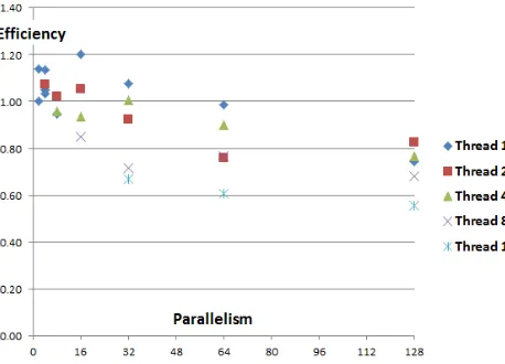
MapReduce for this problem class [14-17]. Figure 4 illustrates the performance of a clustering (into 138 clusters) of a sample of 200K 74 dimensional vectors coming from a pathology informatics application described by Saltz at the CCDSC 2012 workshop [18]. The code is written in C# and run on a Windows HPC environment on eight 16 core nodes with a gigabit Ethernet connection. One finds for this fixed problem size example, a reasonable speedup with a parallel efficiency that decreases naturally as parallelism increases but can be 80% for 128 way parallel case. MPI is of course always used between nodes and on the node either threading (with Microsoft TPL library) or MPI. This paper is not aimed at an authoritative performance study but as in earlier results [8, 19], one finds better performance with MPI rather than threading in the node (note best 128 way parallel performance has 2 threads inside each of 8 MPI processes on each of 8 nodes). Further Windows has a strange [8, 20] degradation of performance for large memory small core runs (note highest efficiency is 16 way parallel case with 16 MPI processes, each with one thread).
4.2 Speed up by use of the Triangle Inequality
There are various ways of speeding up clustering algorithms and especially Kmeans, with the idea of Elkans [21] being important for cases where the points are in high dimension D. This uses the triangle inequality to reduce the number of distance calculations (which take time that is O(D)) needed. This has applied successfully by Qiu in her Twister Kmeans application and uses inequalities such as:
d(x, k-new) ≥ d(x, k-old) – d(k-new, k-old) (25) d(x, k1-new) ≥ d(k1-new, k2-new) - d(x, k2-new) (26)
Here d is metric distance, x is any point and k-old and k-new label positions of center k at previous and current iteration. k1-new and k2-new label current positions of two centers k1 and k2. Thus for example d(x, k-new) = √(X(x)-Y(k)new)2. In Kmeans we know at one iteration, the nearest center to each point and at next iteration, need to update this. Use of an updated array of lower bounds on d(x, k-old) allows one to rule out many centers as candidates for the best center at next iteration by using (25) or (26) in a calculation that is order O(K) and not O(KD) as in basic method. This approach can be extended to deterministic annealing by modifying equation (12) by multiplying numerator and denominator by d(x, knearest-x)/T where knearest-x is the Kmeans center that is nearest to point x. Then we need only include those
centers k in sum in denominator that satisfy:
εx(k) = d2(x, k) ≤ d2(x, knearest-x) + Cutvalue . T (27)
Where exp( - Cutvalue) is small. We use Cutvalue = 20 (28)
[image:6.612.75.304.81.246.2]Note for large temperature T, the constraint (27) (and its estimate using lower bounds) is very weak but at low temperatures where there are the largest number of centers it can be quite strong. For example in the 74 dimensional example given in figs 4 and 5(b), equations (27) and (28) remove 85% of distance
Figure 4: Parallel Efficiency of clustering of 200K points in 74 dimensions on an 8 node 16 core cluster
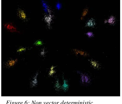
Figure 6: Non vector deterministic annealing clustering and visualization of the “divergent” metagenomics sample with 15761 sequences and 23 clusters [2]
computations averaged over entire run. This work is the first to use the Triangle Inequality with deterministic annealing.
4.3 Parallelism over Centers
The idea of the previous subsection fundamentally changes the problem structure as now each center is associated with its own set of clusters – those near it in sense of equations (27) and (28). Correspondingly each center is only associated with the points near it and the basic parallel model of global reductions still works but may not be most efficient. One needs a decomposition of points that respects the geometric structure and “nearest neighbor communication. Further in this case one can introduce parallelism over centers as those far apart are totally independent. I implemented this for a D=2 problem with 241605 points [1] where as seen in figure 5(left) a simple one dimensional decomposition was efficient. This was implemented with center parallelism and nearest neighbor communication and was a factor of 3 faster than original algorithm which just used the ideas of subsections 4.1 and 4.2. This was a useful gain but not clearly “worth it” as resultant code and approach was much less elegant and general. Note this center parallel approach has similar features to particle in the cell or mesh codes; namely one has two geometric structures – centers and points for clustering – which do not have completely compatible decompositions. The decomposition into equal number of points (near each other) in each node does not have equal number of centers in each node. I believe this approach is first introduced in this paper.
5
Visualization and Dimension Reduction
Clearly clustering needs both to be performed and a measure of quality and confidence developed. One can calculate cluster centers (even in non vector case), cluster sizes and inter-cluster distances. However visualizing the result is a powerful approach and this needs a special approach unless D=2 or 3 when direct display is possible. Otherwise one needs to map system into 3 dimensions for easy visualization. We have developed a suite ofpowerful parallel codes to perform this [22] where the well-known multidimensional scaling is very powerful HMDS = Σx<y=1N weight(x,y) (δ(x, y) – d3D(x, y))2 (29)
[image:7.612.84.279.485.651.2]Here x and y separately run over all points in the system, δ(x, y) is distance between x and y in original space while d3D(x, y) is distance between them after mapping to 3 dimensions. One needs to minimize (29) for optimal choices of mapped positions X3D(x).
Figure 5: Cluster visualizations. (Left) Small portion of 241605 point 2D clustering showing a few “sponge points” (orange) and cluster centers (triangles). (Right) 200,000 74D points with 138 clusters and centers as colored spheres of size proportional to # points in cluster.
Sample results are shown in figures 5 and 6. Note non vector examples can preserve their structure well after mapping (figure 6) while figure 5(right) shows that when there is no dramatic intrinsic structure, clustering ends up similar to break up of region into geometrically compact sub regions. This is a powerful concept as shown for example in recent use of Kmeans in “deep learning” [23].
6
Remarks
Although I have described the vector space case, exactly the same issues are present in non vector case [8, 22] with significantly more complex algebra for formulae like equation (18). There are still many important issues to be explored especially following up discussion in sections 4.2 and 4.3. For the O(N2) non vector methods, we are pursuing much faster hierarchical approaches [2, 24].
7
Acknowledgements
Our work is partially supported by Microsoft and by the NSF under the FutureGrid Grant No. 0910812. I would like to thank Judy Qiu for discussions on material in section 4.2 and D. Mani, and Saumyadipta Pyne for access to data in [10] and to Joel Saltz and Tahsin Kurc for test 74 dimension pathology data.
8
References
1. Rudolf Fruhwirth, D. Mani, and Saumyadipta Pyne, Clustering with position-specific constraints on variance: Applying redescending M-estimators to label-free LC-MS data analysis. BMC Bioinformatics, 2011. 12(1): p. 358. http://www.biomedcentral.com/1471-2105/12/358
2. Yang Ruan, Saliya Ekanayake, Mina Rho, Haixu Tang, Seung-Hee Bae, Judy Qiu, and Geoffrey Fox, DACIDR: Deterministic Annealed Clustering with Interpolative Dimension Reduction using Large Collection of 16S rRNA Sequences, in ACM Conference on Bioinformatics, Computational Biology and Biomedicine (ACM BCB). October 7-10, 2012. Orlando, Florida.
http://grids.ucs.indiana.edu/ptliupages/publications/DACIDR_camera_ready_v0.3.pdf. 3. R open source statistical library. [accessed 2012 December 8]; Available from:
http://www.r-project.org/.
4. Ken Rose, Deterministic Annealing for Clustering, Compression, Classification, Regression, and Related Optimization Problems. Proceedings of the IEEE, 1998. 86: p. 2210--2239.
5. Hofmann, T. and J.M. Buhmann, Pairwise Data Clustering by Deterministic Annealing. IEEE Transactions on Pattern Analysis and Machine Intelligence, 1997. 19(1): p. 1-14.
6. Ken Rose, Eitan Gurewitz, and Geoffrey Fox, A deterministic annealing approach to clustering. Pattern Recogn. Lett., 1990. 11: p. 589--594.
7. Kenneth Rose, Eitan Gurewitz, and Geoffrey C Fox, Statistical mechanics and phase transitions in clustering. Phys. Rev. Lett., Aug, 1990. 65: p. 945--948.
8. Geoffrey Fox, Seung-Hee Bae, Jaliya Ekanayake, Xiaohong Qiu, and H. Yuan, Parallel Data Mining from Multicore to Cloudy Grids. book chapter of High Speed and Large Scale Scientific Computing. 2009: IOS Press, Amsterdam.
http://grids.ucs.indiana.edu/ptliupages/publications/CetraroWriteupJune11-09.pdf. ISBN:978-1-60750-073-5
9. Geoffrey C. Fox, Large scale data analytics on clouds, in Proceedings of the fourth international workshop on Cloud data management. 2012, ACM. Maui, Hawaii, USA. pages. 21-24.
http://grids.ucs.indiana.edu/ptliupages/publications/CloudDB12.pdf. DOI: 10.1145/2390021.2390026.
10. Makoto Yasuda, Deterministic Annealing Approach to Fuzzy C-Means Clustering Based on Entropy Maximization. Advances in Fuzzy Systems, 2011. 2011: p. 9.
DOI:10.1155/2011/960635. http://dx.doi.org/10.1155/2011/960635
11. Hansjorg Klock and Joachim M. Buhmann, Data visualization by multidimensional scaling: a deterministic annealing approach. Pattern Recognition, April, 2000. 33(4): p. 651-669. DOI:http://dx.doi.org/10.1016/S0031-3203(99)00078-3
12. Hansjörg Klock and Joachim M. Buhmann, Multidimensional scaling by deterministic annealing, Chapter in ENERGY MINIMIZATION METHODS IN COMPUTER VISION AND PATTERN RECOGNITION. 1997, Springer Lectures Notes in Computer Science. p. 245-260.
13. Rudolf Fruhwirth and Wolfgang Waltenberger, Redescending M-estimators and Deterministic Annealing, with Applications to Robust Regression and Tail Index Estimation. AUSTRIAN JOURNAL OF STATISTICS, 2008. 3 & 4: p. 301–317.
14. Bingjing Zhang, Yang Ruan, Tak-Lon Wu, Judy Qiu, Adam Hughes, and Geoffrey Fox, Applying Twister to Scientific Applications, in CloudCom 2010. November 30-December 3, 2010. IUPUI Conference Center Indianapolis.
http://grids.ucs.indiana.edu/ptliupages/publications/PID1510523.pdf.
15. J.Ekanayake, H.Li, B.Zhang, T.Gunarathne, S.Bae, J.Qiu, and G.Fox, Twister: A Runtime for iterative MapReduce, in Proceedings of the First International Workshop on MapReduce and its Applications of ACM HPDC 2010 conference June 20-25, 2010. 2010, ACM. Chicago, Illinois. http://grids.ucs.indiana.edu/ptliupages/publications/hpdc-camera-ready-submission.pdf.
16. Thilina Gunarathne, Tak-Lon Wu, Judy Qiu, and Geoffrey Fox, MapReduce in the Clouds for Science, in CloudCom 2010. November 30-December 3, 2010. IUPUI Conference Center Indianapolis.
http://grids.ucs.indiana.edu/ptliupages/publications/CloudCom2010-MapReduceintheClouds.pdf.
17. Thilina Gunarathne, Bingjing Zhang, Tak-Lon Wu, and Judy Qiu, Scalable Parallel Computing on Clouds Using Twister4Azure Iterative MapReduce Future Generation Computer Systems 2012. To be published.
http://grids.ucs.indiana.edu/ptliupages/publications/Scalable_Parallel_Computing_on_Clouds_Us ing_Twister4Azure_Iterative_MapReduce_cr_submit.pdf
18. Clusters, Clouds, and Data for Scientific Computing Workshop CCDSC 2012. [accessed 2012 December 10]; September 11th – 14th, 2012; Châteauform’, La Maison des Contes, 427 Chemin de Chanzé, France Available from: http://web.eecs.utk.edu/~dongarra/CCGSC-2012/index.htm. 19. Judy Qiu and Seung-Hee Bae, Performance of Windows Multicore Systems on Threading and
MPI Concurrency and Computation: Practice and Experience, 2011. Special Issue for FGMMS Frontiers of GPU, Multi- and Many-Core Systems 2010(To be published).
http://grids.ucs.indiana.edu/ptliupages/publications/CCPESpecialIssue_PerformanceofWindows MulticoreSystemsonThreadingandMPI.pdf
20. Geoffrey Fox, Xiaohong Qiu, Scott Beason, Jong Youl Choi, Mina Rho, Haixu Tang, Neil Devadasan, and Gilbert Liu, Biomedical Case Studies in Data Intensive Computing, in The 1st International Conference on Cloud Computing (CloudCom 2009). December 1-4, 2009, Springer Verlag LNCS: Vol. 5931. Beijing Jiaotong University, China.
http://grids.ucs.indiana.edu/ptliupages/publications/SALSACloudCompaperOct10-09.pdf. 21. Charles Elkan, Using the triangle inequality to accelerate k-means, in TWENTIETH
INTERNATIONAL CONFERENCE ON MACHINE LEARNING, Tom Fawcett and Nina Mishra, Editors. August 21-24, 2003. Washington DC. pages. 147-153.
22. Geoffrey C. Fox, Deterministic annealing and robust scalable data mining for the data deluge, in Proceedings of the 2nd international workshop on Petascale data analytics: challenges and opportunities. 2011, ACM. Seattle, Washington, USA. pages. 39-40.
http://grids.ucs.indiana.edu/ptliupages/publications/pdac24g-fox.pdf. DOI: 10.1145/2110205.2110214.
23. Adam Coates and Andrew Y. Ng, Learning Feature Representations with K-means, Chapter in Neural Networks: Tricks of the Trade, 2nd edn, G. Montavon, G. B. Orr, and K.-R. Muller, Editors. 2012, Springer Lecture Notes in Computer Science.
http://www.stanford.edu/~acoates//papers/coatesng_nntot2012.pdf.
24. Judy Qiu, Jaliya Ekanayake, Thilina Gunarathne, Jong Youl Choi, Seung-Hee Bae, Yang Ruan, Saliya Ekanayake, Stephen Wu, Scott Beason, Geoffrey Fox, Mina Rho, and Haixu Tang, Data Intensive Computing for Bioinformatics, Chapter in Data Intensive Distributed Computing, Tevik Kosar, Editor. 2011, IGI Publishers.
http://grids.ucs.indiana.edu/ptliupages/publications/DataIntensiveComputing_BookChapter.pdf.