On-orbit assembly using superquadric potential fields

On-Orbit Assembly Using Superquadric Potential Fields

Ahmed Badawy1 and Colin R. McInnes2 University of Strathclyde, Glasgow, G1 1XJ, UK

The autonomous on-orbit assembly of a large space structure is presented using a method based on superquadric artificial potential fields. The final configuration of the elements which form the structure is represented as the minimum of some attractive potential field. Each element of the structure is then considered as presenting an obstacle to the others using a superquadric potential field attached to the body axes of the element. A controller is developed which ensures that the global potential field decreases monotonically during the assembly process. An error quaternion representation is used to define both the attractive and superquadric obstacle potentials allowing the final configuration of the elements to be defined through both relative position and orientation. Through the use of superquadric potentials, a wide range of geometric objects can be represented using a common formalism, while collision avoidance can make use of both translational and rotation maneuvers to reduce total maneuver cost for the assembly process.

Nomenclature

A = repulsive potential amplitude

Ao = maximum repulsive potential amplitude

a, b, c = superquadratic shape parameters in xB, yB, and zB directions C1, C2 = control gains

a = superquadric parameter vector

⎡

a b c ε₁ ε₂

⎤

T

D = relative Euclidian distance between two superquadric centers d = distance between two superquadric objects

F = superquadric inside-outside function f1 = superquadric scaling function in xB-direction f2 = superquadric scaling function in yB-direction f3 = superquadric scaling function in zB-direction I = element inertia matrix

m = total number of objects in the workspace n = superquadric contour parameter

q = error quaternion vector

⎡

q1 q2 q3 q4

⎤

T

q = part of error quaternion vector

⎡

q1 q2 q3

⎤

T

R = orbit radius

r = object position vector

1

Graduate Student, Department of Mechanical Engineering, [email protected]

2

rG = goal point position vector

s(t) = local (orbital) frame state vector T = control torque vector

t = time

V = global potential field Vatt = total attractive potential

Vatt,rot = attractive rotational potential

Vatt,trans = attractive translational potential

Vobs = obstacle potential

vmax = maximum controlled velocity v = velocity vector

x = element state vector

⎡

x y z q1 q2 q3 q4

⎤

T xB, yB, zB = Cartesian coordinates in body frame of reference xI, yI, zI = Cartesian coordinates in inertial frame of reference xl, yl, zl = Cartesian coordinates in local orbiting frame of reference

= superquadric obstacle potential shape parameter = braking length-scale

= state transition matrix

ε1, ε2 = superquadric roundness parameters

= element radius

= repulsive potential length-scale = circular orbit angular velocity max = maximum controlled angular velocity = object angular velocity vector

I. Introduction

M

any physical systems relax their configuration to attain the lowest possible energy state. This idea has been adopted and used in motion planning algorithms for manipulators and mobile robots as the artificial potential field

method.1 A virtual attractive potential field representing a goal and virtual repulsive potential field representing

obstacles are summed to generate a global potential field, the gradient of which in principle provides a collision-free

path to the goal. The method is widely used for autonomous mobile robot path planning in fixed workspaces where

both target and obstacles are stationary. Extensions to the potential field method due to obstacle and goal position

motion have also been presented through the definition of a velocity dependent potential function.2 Superquadric

potential fields have been introduced for manipulator obstacle avoidance in order to accurately capture the precise

geometric form of obstacles.3 Superquadrics can be used to represent a wide range of geometric objects using the

same common formalism. The potential field method has also been developed for space applications in areas such as

proximity maneuvering,4 large angle slew maneuvers,5 formation-flying6, and autonomous and distributed motion

planning for satellite swarm.7 Other work has focused on the assembly of large, complex space structures using

extensions of the potential field methodology. Here the adjacency matrix of the graph of the final structure is used to

required. A related approach has been used for the autonomous assembly of a group of homogeneous components

by defining and summing vector fields which capture sets of behaviors. The final configuration of the system is

defined by the equilibrium state of the dynamical system formed by the vector fields, in a similar manner to the

global minimum of an artificial potential field.9

As noted above, the artificial potential field methodology is based on the assumption of the existence of a virtual

potential field which attracts maneuvering objects toward a goal, while repelling them away from both static

obstacles and other maneuvering objects. There are strong analogies with physical scalar potential fields which

represent the electric field from electrostatic charges. The gradient of the artificial scalar potential field forms a

vector field which then defines the motion of maneuvering objects in the workspace. While the methodology is

appealing due to its intuitive nature and computationally efficient implementation (controls are typically available in

analytic form), there is often no guarantee that local minima are not present which may trap the maneuvering objects

in some configuration other than the desired one.2 This problem can be overcome by generating the potential field as

a numerical solution to the Laplace equation,4 or by various heuristics such as adding noise to escape form any local

minima. As will be seen, superquadric obstacle representations provide potential surfaces which are largely

symmetrical away form the obstacles, reducing the possibility that local minima may form. More importantly, since

all maneuvering objects are in relative motion simultaneously, even if an object is caught in a temporary local

minimum, it will be displaced due to the motion of other objects perturbing the potential field.

Superquadric functions provide an efficient and flexible means of representing geometric shapes, overcoming

the deficiencies of other representations such as spherically symmetric Gaussian or power law functions where

objects are represented as spheres of diameter equal to the maximum physical object dimension. Rather than a

simple spherical form, the superquadric potential can be moulded to represent the geometric shape of an object by

attaching the potential to the object body axes. In this way the obstacle potential becomes a function of both the

obstacle position and its orientation, unlike previous methods that de-couple translation and rotation.

Transformations with quaternion parameters are then used to define the element superquadric obstacle potentials in

an inertial frame which are then summed together in addition to the attractive goal potential. The global potential

field is then a function of both the position and orientation of the maneuvering objects. This allows collision

avoidance by both translation and rotation, allowing more precise maneuvering than is possible using spherically

assembly of a set of heterogeneous components into a truss-like structure. Other applications include the formation

and re-configuration of symmetric patterns of spacecraft for formation-flying applications where collision-avoidance

can make use of both translation and rotation.

II. Attractive Potential Field

The attractive potential field is a function defined with the goal position at its global minimum. A maneuvering

object will then move down the gradient of the potential field towards this global minimum, and with a suitable

dissipation function will come to rest. In this paper the goal configuration will be defined by both a goal position and

orientation. The Euclidean distance between a maneuvering object and the goal position is used to define the

translational attractive potential while error quaternions are used to define a rotational attractive potential. In order to

reach the global minimum of the attractive potential field, both a final position and orientation must be achieved. In

the subsequent analysis it will be assumed that continuous torques are available for attitude control and that discrete

impulses are available for translational control. This is similar to the configuration of agile robot free-flyers which

use control moment gyros and pulsed thrusters for actuation.

The overall attractive potential is the summation of both the translational and rotational attractive potentials. The

translational attractive potential aims to null the Euclidian distance between a maneuvering object and its goal

position, while the rotational attractive potential aims to bring the error quaternion to , relative to the

required final orientation. The attractive potential guides each extended maneuvering object toward its goal

configuration, both in position and orientation through impulsive velocity changes and continuous torque

commands. The attractive potential is therefore defined as:

⎡

T

1 0 0

0

⎤

rot , att trans , att

att V V

V = +

( )

q q I

r

r T T

G

att C

V

2 1 2

1

1 2

+ +

−

= (1)

Adding a translational potential to a rotational potential in a single global potential field leads to full 6

degree-of-freedom maneuvering control, as will be seen later. The controller is able to choose between translation and/or

rotation to reach its goal and most importantly, with the addition of repulsive obstacle potentials will allow

In order to ensure a continuous approach to the goal, the required maneuvering object velocity vector may be

chosen to be directed along the gradient of the potential at every point in the workspace. Therefore, the required

maneuvering object velocity vector v can be expressed as:11

att att

V

V

k

∇

∇

−

=

v

if V&≥0

G G

k

r

r

r

r

−

−

−

=

(2)

so that an impulse is applied if , otherwise control intervention is not required if the maneuvering object

is already moving towards the goal such that . An exponential time approach is guaranteed if

0

V

&

≥

0

V

&

<

(

Vatt

)

max

e

v

k

=

1

−

−β for some maximum translational speed vmax and braking parameter β. For maneuvering

towards a single goal with no obstacles, motion planning then becomes a stability problem through the use of

Lyapunov’s theorem. If the dynamical system formed by the global potential field is shown to be stable the

maneuvering object will reach its goal. The time derivative of the function Vatt is expressed as:

(

r

r

)

( )

q

q

I

v

&

T T

&

&

₌

₋

₊

₊

1

2

C

V

_att T _G (3)

However, the first derivative of the quaternion is defined as:12

Q q

2 1 =

& ₍₄₎

where Q is the matrix of quaternion components and is defined in the usual manner as:

(5) ⎥

⎥ ⎥ ⎦ ⎤ ⎢

⎢ ⎢ ⎣ ⎡

− −

− =

4 1 2

1 4 3

2 3 4

q q q

q q q

q q q Q

Substituting for the quaternion kinematics in Eq (3) it can be seen that

(

r r

)

Q q I

v T T T &

& _{= − + +}

1 C

V_att T _G

and so we have QTq=q4q such that:

(

r r

)

(

q I

)

v T &

& _{= − + +}

4 1

V_att T _G Cq (7)

Euler's equation defines the external torque T acting on the rigid body as:

I I

T= &+ × (8)

Hence;

(

r r

)

(

q T I

)

v − + T + − ×

= C₁q₄

V&_att T _G (9)

A linear control torque will now be defined such that T=−C₁q₄q−C₂ and so:

(

r r

)

(

I

)

v − + T − − ×

= ₂

V&_att T _G C (10)

However, it is clear that T

(

×I

)

=0 so that:

(

r r

)

v ₂ T

V&att = T − G −C (11)

Using Eq. (2) it is then concluded from Eq. (11) that is satisfied for all states except the goal position, so

that the proposed attractive potential function can be considered as a Lyapunov function where:

0 V&att<

0

V&_att ≤−kr−r_G −C₂ T ≤ (12)

With the definition of the attractive potential field, the addition of obstacles through the use of superquadric

potential can now be considered. By attaching the superquadric potential to the object body axes, translation and

rotational motion will then become strongly coupled, allowing precise maneuvering for collision avoidance

III. Superquadric Obstacle Representation

Superquadrics are a family of complex geometric objects which include superellipsoids and superhyperboloids.

The geometric object which will be used here is the superellipsoid, which may be referred to with the general term

superquadric.13 Superquadrics are mathematical representations of solid objects. They are a set of parametric

object shapes by manipulating the so-called roundness and shape parameters. A generic superquadric function is

defined in body axes as:

1 1 1 2 2 2 2 2 2 = ⎟ ⎠ ⎞ ⎜ ⎝ ⎛ + ⎥ ⎥ ⎥ ⎦ ⎤ ⎢ ⎢ ⎢ ⎣ ⎡ ⎟ ⎠ ⎞ ⎜ ⎝ ⎛ + ⎟ ⎠ ⎞ ⎜ ⎝

⎛ ε ε

ε ε ε c z b y a

x_{B B B}

(13)

The inside-outside function F defines whether a point lies inside, on the surface or outside a superquadric surface

and is given by:14

(

)

1

1 2 2 2 2 2 2 ε ε ε ε ε _⎟ ⎠ ⎞ ⎜ ⎝ ⎛ + ⎥ ⎥ ⎥ ⎦ ⎤ ⎢ ⎢ ⎢ ⎣ ⎡ ⎟ ⎠ ⎞ ⎜ ⎝ ⎛ + ⎟ ⎠ ⎞ ⎜ ⎝ ⎛ = c z b y a x ,

F axB B B B (14)

Consider any point P with coordinates (xB,yB,zB) with respect to a set of body axes attached to the superquadric. If F<1, point P lies inside the superquadric whereas if F=1, the point lies on the superquadric surface, and finally if

F>1, the point lies outside the superquadric. Various obstacle shapes can now be represented using the superquadric methodology by adjusting the five parameters defined in Eq. (13). For example, in order to define a spherical shape

at some distance from the object edges, the shape parameters 1, and 2 should approach unity. The superquadric

form of particular object shapes will be defined and used later for application to the on-orbit assembly problem. As

will be seen, through the appropriate choice of shape parameters the precise geometric form of objects can be

captured in proximity to them, but smoothed away from the object to allow for collision avoidance with less

likelihood of local minima formation.

A. Parallelepiped Obstacle (Cuboid)

The parallelepiped shape is common in structural assembly problems. A wide range of elements can be modeled

by manipulating the superquadric parameters. Columns and plates can be modeled by fixed parameters, while

triangles and trapezoids can be modeled by a variable set of parameters. Parallelepiped obstacles were first

investigated by Volpe as static objects for collision avoidance during manipulator control.15

To form a parallelepiped shape the values of ε1 and ε2 are chosen to approach zero in proximity to the object to

to form a smooth ellipsoid. Figure 1 shows a superquadric model for such a cuboid element. The most general form

of an implicit function for a parallelepiped object is defined as:

(

)

(

)

(

)

1

, , , , , , 2 3 2 2 2 1 = ⎟⎟ ⎠ ⎞ ⎜⎜ ⎝ ⎛ + ⎟⎟ ⎠ ⎞ ⎜⎜ ⎝ ⎛ + ⎟⎟ ⎠ ⎞ ⎜⎜ ⎝ ⎛ n B B B B n B B B B n B B B B z y x f z z y x f y z y x f x (15)

where the scaling functions f are used to define the required geometric form of the parallelepiped.

For example, the scaling functions for a column and a plate are constants. They can then be set to a, b, and c, the

semi major axis in xB, yB, and zB directions respectively such that:

1 2 2 2 = ⎟ ⎠ ⎞ ⎜ ⎝ ⎛ + ⎟ ⎠ ⎞ ⎜ ⎝ ⎛ + ⎟ ⎠ ⎞ ⎜ ⎝

⎛ B n

n B n B c z b y a x (16)

It is now possible to modify the nested level surfaces defined by Eq. (16) to form a sphere away from the object

rather than an ellipsoid by adjusting the coefficients as:

1 2 2 2 2 2 = ⎟ ⎠ ⎞ ⎜ ⎝ ⎛ ⎟ ⎠ ⎞ ⎜ ⎝ ⎛ + ⎟ ⎠ ⎞ ⎜ ⎝ ⎛ ⎟ ⎠ ⎞ ⎜ ⎝ ⎛ + ⎟ ⎠ ⎞ ⎜ ⎝

⎛ B n

n B n B c z a c b y a b a x (17)

The inside-outside function is then expressed as:

(

)

B n

n B n B B c z a c b y a b a x , F 2 2 2 2 2 ⎟ ⎠ ⎞ ⎜ ⎝ ⎛ ⎟ ⎠ ⎞ ⎜ ⎝ ⎛ + ⎟ ⎠ ⎞ ⎜ ⎝ ⎛ ⎟ ⎠ ⎞ ⎜ ⎝ ⎛ + ⎟ ⎠ ⎞ ⎜ ⎝ ⎛ = x

a (18)

Deformable superquadric surfaces are represented by introducing a new shaping parameter, n, related to each

surface. This parameter replaces both ε1 and ε2 with the value of n ∞ near the object edges (to ensure sharp edges)

while n 1 away from the object (to ensure smoothness) to form an n-ellipsoid with semi-axes a, b, and c. Following Vople, n can be defined as:16

d

e

n _−α

− =

1 1

(19)

The parameter has a major influence on the potential field and the transition from sharp to smooth potential

surfaces. The parameter α determines both the sharpness of the object potential shape and the transition from the

actual obstacle shape to a spherical shape at large distance. Increasing the value of increases the sharpness of the

of the object shape to influence the potential field at large distances from the object. By changing its value the

influence of object edges can be manipulated to overcome the formation of any local minima which may form when

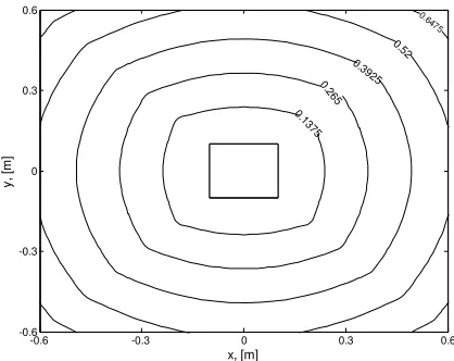
dealing with multiple objects. Figure 1 shows the effect of on the object iso-potential contours.

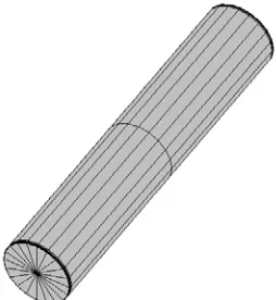
B. Cylindrical Obstacle (Beam)

Beam elements are again widely used in structural assembly problems, especially in truss-type structures.

Cylinders can be represented by a superquadric function by setting the shape parameter ε1 0, and ε2 = 1. Figure 2a

shows a superquadric model for a cylindrical element.

The objective of having spherical symmetry away from the obstacle edges will be guaranteed by deforming the

superquadric shape from a cylinder to a sphere. For a spherical shape both ε1 and ε 2 should be set to unity, hence the

parameter ε2 will remain unchanged throughout the workspace, while the parameter ε1 should be gradually changed

from zero at the beam edge to unity. It is then inversely proportional to the contour parameter n. Hence, the

superquadric model can be adapted to the following form as:

1 2 2 2 2 = ⎟ ⎠ ⎞ ⎜ ⎝ ⎛ ⎟⎟ ⎠ ⎞ ⎜⎜ ⎝ ⎛ + ⎥ ⎥ ⎦ ⎤ ⎢ ⎢ ⎣ ⎡ ⎟⎟ ⎠ ⎞ ⎜⎜ ⎝ ⎛ + ⎟⎟ ⎠ ⎞ ⎜⎜ ⎝ ⎛ n B n B B c z c y x ρ ρ

ρ (20)

for a cylinder of radius ρ. The corresponding inside-outside function is then expressed as:

(

)

B n

n B B B c z c y x , F 2 2 2 2 ⎟ ⎠ ⎞ ⎜ ⎝ ⎛ ⎟⎟ ⎠ ⎞ ⎜⎜ ⎝ ⎛ + ⎥ ⎥ ⎦ ⎤ ⎢ ⎢ ⎣ ⎡ ⎟⎟ ⎠ ⎞ ⎜⎜ ⎝ ⎛ + ⎟⎟ ⎠ ⎞ ⎜⎜ ⎝ ⎛ = ρ ρ ρ x

a (21)

The beam element iso-potential contours are shown in Fig. 2. The iso-potentials in the circular cross-section

plane remains unchanged, whereas those in the longitudinal plane change their shape in the same way as those of the

cuboid element to provide sharp edges close to the beam and a smooth symmetric potential far from the beam.

IV. Obstacle Potential Field

The formulation of the obstacle potential field from the individual obstacles depends on the behavior required

whilst approaching an obstacle. Two types of repulsive potential fields are used: the avoidance potential field and

the approach potential field, as defined by Volpe15. Each is defined over a certain distance around the obstacle. The

obstacles. This is achieved by introducing a repulsive potential around the obstacle which is sufficient to force the

controlled object to move away from the obstacle regardless of the kinetic energy of each of them. The best way to

ensure this requirement is to define infinite repulsive potential in the avoidance potential region. The minimum

distance between any two superquadric object surfaces, an obstacle at xB,obs and a maneuvering object at xB,obj, can be determined from the distance D between their geometric centers. This is found to be:17

(

)

(

)

⎥

⎦ ⎤ ⎢

⎣ ⎡

− −

=D F obs, B,obs −n F obj, B,obj −n

d 2

1 2

1

1 a x a x (22)

The avoidance potential is then calculated through the use of the so-called Born approximation for a Yukawa

potential in which the exponential term reaches zero faster than the inverse distance term as18:

(

)

d d exp A Vobs

α

−

= , d ≥ dmin (23)

The objective of the approach potential is to decrease the kinetic energy of the maneuvering object when

approaching the obstacle within a certain distance to reduce the approach velocity and to generate smooth contact

between objects. Smooth contact is clearly required in the goal position to achieve the final contact for mechanical

assembly. The approach potential function can then be expressed as:

⎟ ⎟ ⎠ ⎞ ⎜

⎜ ⎝ ⎛ −

= _α +α

1 1 d exp A

V_obs , d < dmin (24)

The repulsive potential amplitude, A, is used to define the maximum repulsive potential between objects. This

amplitude should be defined depending on the maximum allowable translational velocity of the objects. The

parameter A is crucial for structural assembly problems as it is expressed as a function of the configuration of the

objects. Allowing the obstacle potential to vanish at the goal configuration allows smooth contact, which is again

required for connection of the elements for assembly.19 The repulsive amplitude may then be expressed as a smooth

Gaussian function as:

(

)

(

2 σ

)

1− −r−rG

=A exp

A _o (25)

so that mechanical contact can be made as the maneuvering objects reach their goal. The global potential field

V. Global Potential Field

The global potential is a linear superposition of the attractive and repulsive potentials, as shown in Fig. 3 for a

single object. However, different potentials must be defined with respect to the same frame of reference. Although,

each superquadric obstacle function is expressed in a body frame attached to the obstacle, only the distances

between them are required to calculate the obstacle potential function. Object coordinates are therefore transformed

from an inertial frame to a body frame through a homogeneous transformation. This operation is well established by

using quaternions as:

(

)

(

)

(

)

(

)

(

)

(

)

obj obs _I

obs obj obs obj 2 4 2 3 2 2 2 1 2 4 2 3 2 2 2 1 2 4 2 3 2 2 2 1

B z z

y y x x q q q q q q q q 2 q q q q 2 q q q q 2 q q q q q q q q 2 q q q q 2 q q q q 2 q q q q z y x 4 1 3 2 4 2 3 1 4 1 3 2 4 3 2 1 4 2 3 1 4 3 2 1 ⎥ ⎥ ⎥ ⎦ ⎤ ⎢ ⎢ ⎢ ⎣ ⎡ − − − ⎥ ⎥ ⎥ ⎥ ⎦ ⎤ ⎢ ⎢ ⎢ ⎢ ⎣ ⎡ + + − − − + + + − + − − − + + − − = ⎥ ⎥ ⎥ ⎦ ⎤ ⎢ ⎢ ⎢ ⎣ ⎡ (26)

The quaternion parameters in Eq. (26) are the actual quaternion parameters which orient the object, unlike those

in the attractive potential which are error quaternions. Transformation between the two types of quaternions is

carried out through the following equation:

(27) error goal q q q q q q q q q q q q q q q q q q q q q q q q ⎥ ⎥ ⎥ ⎥ ⎥ ⎤ ⎢ ⎢ ⎢ ⎢ ⎢ ⎡ ⎥ ⎥ ⎥ ⎥ ⎦ ⎤ ⎢ ⎢ ⎢ ⎢ ⎣ ⎡ − − − − − − = ⎥ ⎥ ⎥ ⎥ ⎥ ⎤ ⎢ ⎢ ⎢ ⎢ ⎢ ⎡ 4 3 2 1 4 3 2 1 3 4 1 2 2 1 4 3 1 2 3 4 4 3 2 1

Substituting the local coordinates produced from Eq. (26) in conjunction with Eqs. (19) and (21) in Eq. (22), the

distance between any two objects is calculated and consequently the obstacle potential is fully defined. The addition

of different potential functions may result in some issues such as:

i) Local minimum due to the interference between spherically symmetric attractive potentials and obstacle

potentials produced with sharp edges.

ii) Local minimum due to the existence of multiple obstacles close to each other.

iii) The "goal non-reachable due to obstacle nearby" problem which exists when an obstacle is located near the

goal position. Consequently the global minimum of the potential field may be shifted from the desired location.

However, all these problems were in fact found to be overcome through the use of the superquadric obstacle

approaching the goal configuration. The overall potential field of a maneuvering object i in the presence of m-1

obstacles is now defined as:

For di,j≥ dmin

(

)

(

)

∑ ≠ = − + + + − = m i j ,

j i,j i j

, d i i i T i i T i i, G i i , d e A C V j i j , i 1 1 2 2 1 2 1 r r a, I q q r r r r a, α (28)

and for di,j < dmin

(

)

∑ ≠ = − + + + + − = m i j , j , d i i i T i i T i i, G i

i C A e i,j i j

V 1 1 2 1 1 2 1 2

1 α a,rr α

I q

q r

r (29)

Therefore, the required kinematics for object i in the presence of m-1 obstacles through continuous approach to

the goal is provided in the same way used to determine object velocity with the absence of obstacles as discussed in

section II. The required translational velocity is found to be:

(

)

(

)

i * m i i, j j , i j , i obs G i V max i V d d V e v j , i i i , att ∇ ∇ ∂ ∂ + − − − =

∑

≠ = − 1 1 r r

v β (30)

while the control torques can be determined from the quaternion kinematics as

(

)

i * m i j , j j , i q j , i obs i T i V max i V d d V C e j , i i, att ∇ ∇ ∂ ∂ + − − =

∑

≠ = − 1 1 2 1 q q q &

& _ω β ₍₃₁₎

(

)

−1 i i i i , i

i=−I C1q 4q +C2 + ×I

& , q&i,4=−qiTq&i qi,4

I I T (32) i i i

i = & + × (33)

where ∇=

⎡

∂ ∂x ∂ ∂y ∂ ∂z

⎤

T (34-a)

⎡

∂ ∂q1 ∂ ∂q2 ∂ ∂q3 =

∇q

_⎤

T

(34-b)

⎡

∂ ∂x ∂∂y ∂ ∂z ∂∂q1 ∂ ∂q2 ∂∂q3 =

∇*

_⎤

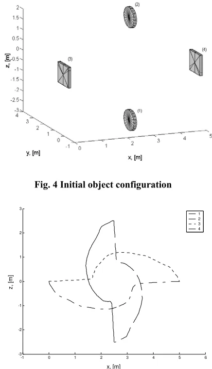
T _(34-c)

The following example shows the simultaneous motion of four objects: two parallelepipeds of dimensions 1 x 1

x 0.1 m and of 1 kg mass and two discs of 1 m diameter, 0.1 m thickness and 1.2 kg mass. The maximum controlled

maneuvers will be replaced by rotational maneuvers when the objects are in close proximity. The repulsive

parameters are defined as = 1, Ao = 4, = 0.1, and = 1. The control law parameters, C1 and C2, are selected as

unity. Each pair of identical objects will switch their location to demonstrate the interaction between the

translational and rotational potential fields. The obstacle avoidance potential fields demonstrate how objects of

different shapes can be modeled using superquadric functions. Due to the formulation of the control method, the

objects choose between translation and/or rotation in order to reduce the global potential function and so reach their

goals. The initial object configuration is shown in Fig. 4, while the translational maneuvers and error quaternion

parameters are shown in Fig.5. Figure 6 shows the objects during the maneuver.

The interaction between translation and rotation is evident as the objects change their orientation whilst

translating to their respective goals. The ability to simultaneously rotate and translate for collision avoidance is a

novel aspect of the method presented here and arises from the coupling of the translational obstacle potential field to

the orientation of the objects through the use of superquadric potential fields attached the object body axes.

VI. Implementation for On-Orbit Assembly

The previous analysis has shown that the superquadric obstacle representation along with quaternion parameters

for attitude representation can succeed in bringing maneuvering objects to their goals while avoiding mutual

collisions by rotation and translation. Each structural element is now assumed to maneuver as a free-flyer having

translational maneuvers actuated using thrusters (impulsive velocity changes), and rotational maneuvers actuated

using control moment-gyros (continuous torques). On-orbit assembly will be considered in low Earth orbit (LEO) of

altitude 100 km, so that the motion of the maneuvering objects is propagated using linearised orbital dynamics.

A. Equations of Motion:

The equations of motion describing transfer of a maneuvering object from some initial point on a circular orbit

towards a goal are now defined. By considering small distances between the initial position of the maneuvering

objects and their goal positions, the relative motion can be described using the Clohessy-Wiltshire (CW) equations.20

The state transition matrix of the CW equations will propagate the element motion between control impulses.

In this model a structural element is placed in orbit with a reference orbital angular velocity , and position

The linearised equations of motion in a local orbiting frame are then found to be:

L L

x& 2 z&

& =− Ω (35-a)

(35-b) L

L y

y& =−Ω

& 2

2

(35-c) L

L

L z x

z& &

& =3Ω +2Ω

where Ω= GM R3 is the circular orbit angular velocity. The solution to these linear differential equations

describes the maneuvering element motion, with the state transition matrix (t) as:

( )

( ) ( )

s0

st = t (36)

where , and s(0) is the initial conditions for the current period of free flight between impulses. The state transition matrix can then be defined as:

( )

⎡

T

L L L L L

L y z x y z

x

t = & & &

s

⎤

20

( )

( )

(

)

(

( )

)

(

( )

)

( )

( )

( )

(

( )

)

( )

( )

(

)

( )

( )

( )

( )

( )

( )

( )

⎥⎥ ⎥ ⎥ ⎥ ⎥ ⎥ ⎥ ⎥ ⎥ ⎦ ⎤ ⎢ ⎢ ⎢ ⎢ ⎢ ⎢ ⎢ ⎢ ⎢ ⎢ ⎣ ⎡ − − − − − − − − − = t cos t sin t sin t cos t sin t sin t cos t cos t sin t cos t cos t sin t cos t cos t t sin t t sin t Ω Ω Ω Ω Ω Ω Ω Ω Ω Ω Ω Ω Ω Ω Ω Ω Ω Ω Ω Ω Ω Ω Ω ω Ω Ω 0 2 3 0 0 0 0 0 0 2 0 3 4 1 6 0 0 0 1 2 3 4 0 0 0 0 0 0 1 2 0 3 4 1 6 0 1 (37)

B. On-Orbit Assembly

Many future large space structures will be unable to be launched as a single assembly. Carrying unassembled

structural elements in several launch vehicles then assembling them in-orbit will be required for both large

mechanical structures, such as trusses, and for large science missions using multiple spacecraft for formation-flying.

It is assumed that all the elements for the structure are initially on a circular orbit in some initial configuration.

Natural orbital motion can bring the elements toward their goals or away from them, depending on their relative

position and velocity. Therefore, control actuation is required when the global potential field is not monotonically

decreasing and the elements maneuver towards their goal. The only limitation on the initial configuration of the

The artificial potential field can control the assembly process through constructing an attractive potential field

with a global minimum situated in the goal configuration of each element, while the repulsive potential field is used

for collision avoidance. The potential functions, both attractive and repulsive, will be described with respect to the

local, orbiting frame of reference. Control intervention will be used when the rate of change of the global potential

function is larger than some non-positive value. Control actuation is then required when:

(38) f

i c

V& ≥

The control trigger constant, cf, can be set to zero for Lyapunov-like stability, however a negative value can be

used in order to preempt collision avoidance maneuvers. The correct choice of the control constant results in

minimizing the required thruster activity and so minimizing the propellant mass used for the assembly process.

C. On-Orbit Assembly Example

The initial velocities of all the elements to be assembled are set to zero relative to the goal position, hence the

initial rate of change of the potential is zero. As a result, control actuation will be required if cf<0 and so the

assembly process will start. The rate of change of the global potential is found and the control actuation is made

according to Eq. (38).

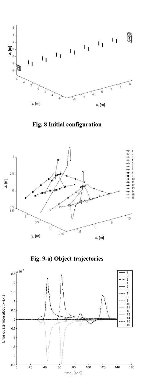
This example considers the assembly process of 14 beams of 0.1 m diameter, 1 m length, and mass of 20 kg and

plates of dimensions 1.2 x 1.2 x 0.3 m and mass of 75 kg, and of dimension 2.2 x 1.2 x 0.5 m and mass of 230 kg.

All objects move under both natural orbital motion and control action with a maximum controlled velocity of 0.1

m/sec and a maximum controlled angular velocity of 0.1 rad/sec. The repulsive parameters are defined as = 7,

Ao = 6, = 0.1, and = 1. The control law parameters, C1 and C2, are selected as unity. The initial configuration of

the objects is shown in Fig. 8, while the object trajectories and error quaternion parameters are shown in Fig. 9. The

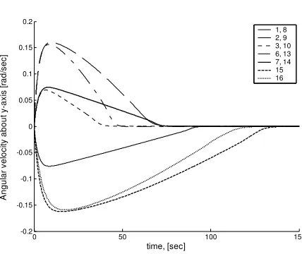
maneuvering object angular velocities are shown in Fig. 10, while Fig. 11 shows the object configuration during the

assembly process, as well as part of their trajectories to illustrate the objects paths. The final assembled truss-like

structure is shown in Fig. 12. The structure requires approximately 150 s to complete the assembly using a

maximum controlled velocity of 0.1 m s-1. The control trigger constant cf was set to zero, since this is the most

D. Cost of Assembly

The assembly cost is measured by the overall ∆v summed from every control action. It is affected by the presence of the obstacle potential of other objects so that a variation in cost for different elements is expected. Cost

optimization could be achieved through the optimal choice of parameters such as the maximum controlled velocity

and control trigger cf defined in Eq. (38), since this represents the threshold at which the controller will act. Figure

13 shows the absolute ∆v for each element, where an initial ∆v of 0.1 m s-1 is delivered to initiate the assembly process by maneuvering the objects towards the goal. Small impulses are required at the end of each object

trajectory to help in the precise coordination between objects to avoid collision and to reach their goals. The

maneuvering object translation costs are shown in Table 1 and are seen to be relatively modest.

Again, the key benefit of the method presented relative to other approaches is the ability to capture the geometric

form of maneuvering objects, unlike spherically symmetric potentials8 and the ability to perform coupled

translational and rotational maneuvers for collision avoidance. This is more flexible than other approaches to

distributed motion planning.7

E. Free-Flying Robots

In order to demonstrate the flexibility of the methodology presented, two free-flying robots, of dimension 0.1 x

0.1x 0.1 m and mass of 0.5 kg, are consider maneuvering in proximity to the structure. The free-flyers are controlled

using the same control parameters as the structural elements. Each free-flyer is affected by the repulsive potentials

of the 16 elements constituting the structure, in addition to the other free-flyer. Figure 15 shows the proximity

motion of the two free-flyers, R1 and R2 who maneuver past each other. Their close maneuvering inside the

structure again demonstrates the flexibility of the method.

F. Structure Reconfiguration

In this example, a hexagonal structure is assembled from 6 beams. All beams are again considered as extended

rigid bodies rather than point masses, as used in previous studies.9 The beam type objects have length 1 m, diameter

0.1 m and a mass of 20 kg mass, and are initially in a parking position with 1 m separation distance, Fig. 16. The

beams are then tasked to perform an extremely complex maneuver to form a closed hexagonal formation without

collision. All control constants are unity, the maximum controlled velocity is 0.02 m sec-1, while the repulsive

parameters are defined as = 6, Ao = 50, = 0.1, and = 1.

During the 400 sec of the first task, strongly coupled translation and rotation maneuvers are performed to from

the initial goal configuration shown in Fig. 17. The total translation costs are shown in Table 2. As the objects are

disengaged, they are repelled due to their mutual repulsive potentials, while later each maneuvers towards its new

configuration. Using the same parameters as in the first phase, the objects are able to reach their new goals and are

assembled together in a line without collision in 200 sec, Fig. 18. The middle objects such as (1) and (4) require

larger impulses and consequently total maneuver cost since they experience a more complex potential field topology

compared with those on the two ends as shown in Table 3.

VII. Conclusion

On-orbit assembly using superquadric potential fields has been presented. The obstacle superquadric potential

field has been attached to each obstacle body axes so that the global potential is a function of both position and

orientation. Interaction between the translational and rotational attractive potential along with that of the obstacles

results in flexibility for the algorithm to choose which behavior, rotation and/or translation, is effective in driving the

assembly process. Various object shapes were used within the algorithm, represented using the superquadric

functions. The obstacle repulsion amplitude was scaled to maintain constant repulsive amplitude for all locations

away from the goal, while decreasing the amplitude close to the goal to allow mechanical contact for assembly.

Simulation shows that complex assembly processes can be undertaken, again with simultaneous rotation and

translation used for collision avoidance between the maneuvering objects. The controls are available in closed,

analytic form allowing computationally efficient, on-board implementation.

References

1

Khatib O., "Real-Time Obstacle Avoidance for Manipulators and Mobile Robots", The International Journal of Robotics

Research, Vol. 5, No. 1, 1986, pp. 90-98.

2

Ge S.S., and Cui Y.I., “Dynamic Motion Planning for Mobile Robots using Potential Field Method”, Autonomous Robots

Vol. 13, No. 3, 2002, pp. 207-222.

3_{Khosla P. and Volpe R., "Superquadric Artificial Potentials for obstacle Avoidance and Approach", IEEE Conference on}

4

Roger, A.B., and McInnes, C.R., “Passive-Safety Constrained Free-Flyer Path-Planning with Laplace Potential Guidance at

the International Space Station”, Journal of Guidance, Control and Dynamics, Vol. 23, No. 6, 2000, pp. 971-979.

5

McInnes C.R., “Potential Function Methods for Autonomous Spacecraft Guidance and Control”, AAS 95-447, AAS/AIAA

Astrodynamics Specialist Conference, Halifax, Canada, August, 1995.

6

McQuade, F., Ward, R., Ortix, F., and McInnes, C.R., “The Autonomous Configuration of Satellite Formations using

Generic Potential Functions”, 3rd International Workshop on Satellite Constellations and Formation-Flying, Italy, February, 2003.

7

Izzo D., Pettazzi L., and Ayre M., "Mission Concept for Autonomous on Orbit Assembly of a Large Reflector in Space",

IAC-05-D1.4.03, 56th International Astronautical Congress, Fukoka, Japan, September, 2005.

8

McQuade, F., and McInnes, C.R., “Autonomous Control for On-Orbit Assembly using Potential Function Methods”, The

Aeronautical Journal, Vol. 101, No. 1008, 1997, pp. 255-262.

9

Izzo D., and Pettazi L., "Autonomous and Distributed Motion Planningfor Satellite Swarm", Journal of Guidance,

Control, and Dynamics, Vol. 30, No. 2, 2007, pp. 449-459.

10

Badawy A., and McInnes C.R., "Autonomous Structure Assembly Using Potential Field Functions", IAC-06-C1.P.3.04,

57th International Astronautical Congress, Valencia, Spain, October, 2006.

11

Casasco M. and Radice G., "Autonomous Slew Maneuvering and Attitude Control using the Potential Function Method",

AAS 03-612, AAS/AIAA Astrodynamics Conference, Big Sky, August, 2003.

12

Wie B., Space Vehicle Dynamics and Control, AIAA Education Series, pp. 307-322, 1998.

13

Barr A., "Superquadrics and Angle-Preserving Transformations", IEEE Computer Graphics and Applications, Vol. 1, No. 1,

pp. 11-23, 1981

14

Solina F. and Bajcsy R., "Recovery of Parametric Models from Range Images: The Case for Superquadrics with Global

Deformations", IEEE Transaction on Pattern Analysis and Machine Intelligence, Vol. 12, No. 2, 1990, pp. 131-147.

15

Volpe R. and Khosla P., " Manipulator Control with Superquadric Artificial Potential Functions: Theory and Experiments",

IEEE Transaction on Systems, Man, and Cybernetics, Vol. 20, No. 6, 1990 pp. 1423-1436.

16_{Volpe R., "Real and Artificial Forces in the Control of Manipulators: Theory and Experiments" Ph. D Dissertation,}

Carnegie Mellon University, 1990.

17

Badawy A., and McInnes C.R., "Separation Distance for Robot Motion Control using Superquadric Obstacle Potentials",

International Control Conference, Glasgow, UK, September, 2006, paper no. 25.

18

Cohen C., Diu B., and Laloë F., Quantum Mechanics, Vol. 2. John Wiley and Sons, New York, 1977, pp. 957-958.

19

McQuade F., "Autonomous Control for On-Orbit Assembly Using Artificial Potential Functions", Ph. D Dissertation,

20

Yu S., "On the Dynamics and Control of the Relative Motion between Two Spacecraft", Acta Astronautica, Vol. 35, No. 6,

Fig. 1-a) Cuboid element representation using a superquadric function

-0.6 -0.3 0 0.3 0.6

-0.6 -0.3 0 0.3 0.6

x, [m]

y,

[

m

]

0.1 37₅

0.2 65

0.3₉₂ 5

0.5₂ 0.6₄₇

5

Fig. 1-b) Cuboid element obstacle iso-potential contours near the obstacle ( = 1)

-0.6 -0.3 0 0.3 0.6

-0.6 -0.3 0 0.3 0.6

x, [m]

y

, [m

]

0.1 39₄₅

0.26₈₉ 0.3₉₈

35 0.5₂₇

8 0.6₅₇

24

[image:20.612.221.414.96.227.2] [image:20.612.205.414.296.462.2] [image:20.612.205.415.513.680.2]

Fig. 2-a) Cylindrical element representation using a superquadric function

-0.6 -0.3 0 0.3 0.6

-0.6 -0.3 0 0.3 0.6

x, [m]

y,

[

m

]

0.14 0.27

0.4 0.5

Fig. 2-b) Beam element obstacle iso-potential contours in circular cross section plane ( = 5)

-2 -1.5 -1 -0.5 0 0.5 1 1.5 2

-2 -1.5 -1 -0.5 0 0.5 1 1.5 2

z,

[

m

]

x, [m]

0.5 1

1.5 2

[image:21.612.254.381.89.227.2] [image:21.612.227.395.296.462.2]

[image:22.612.200.418.295.674.2]

Fig. 3 Global potential function with a single rectangular obstacle

Fig. 4 Initial object configuration

-1 0 1 2 3 4 5 6

-3 -2 -1 0 1 2 3

x, [m]

z,

[

m

]

1 2 3 4

0 100 200 300 400 500 600 -0.6

-0.5 -0.4 -0.3 -0.2 -0.1 0 0.1 0.2 0.3

time, [sec]

Q

ua

ter

n

io

n c

om

pon

ent

a

bou

t y

-a

x

is

1 2 3 4

Fig. 5-b) Quaternion parameters

Fig. 6-a) Object configuration at t = 185 [sec]

[image:23.612.207.419.302.468.2]

Fig. 6-c) Object configuration at t = 272 [sec]

Fig. 6-d) Final object configuration at t = 1000 [sec]

xL goal

R

zBi

zL

roi

i xBi ri

xI

zI

rGi

[image:24.612.205.418.88.256.2]

ri-rGi

[image:24.612.205.417.311.474.2] [image:24.612.202.432.510.675.2]

[image:25.612.197.433.74.698.2]

Fig. 8 Initial configuration

Fig. 9-a) Object trajectories

0 20 40 60 80 100 120 140 160

-2.5 -2 -1.5 -1 -0.5 0 0.5 1 1.5 2 2.5x 10

-3

time, [sec]

E

rr

or

q

uat

er

ni

on

a

bout

x

-axi

s

1 2 3 4 5 6 7 8 9 10 11 12 13 14 15 16

0 20 40 60 80 100 120 140 160 -0.8 -0.6 -0.4 -0.2 0 0.2 0.4 0.6 0.8 time, [sec] E rr o r quat e rni o n abou t y-axi s 1, 8 2, 9 3, 10 4, 11 5, 12 6, 13 7, 14 15 16

Fig. 9-c) Error quaternion about y-axis

40 60 80 100 120 140 160

-8 -6 -4 -2 0 2 4 6 8x 10

-4 time, [sec] E rr o r quat e rni o n abou t z-axi s 1 2 3 6 7 8 9 10 13 14 15 16

Fig. 9-d) Error quaternion about z-axis

0 50 100 150

-6 -4 -2 0 2 4 6x 10

-4 time, [sec] Angul ar v e lo ci ty about x-ax is [ rad/ s e c ] 1 2 3 6 7 8 9 10 13 14 15 16

[image:26.612.194.409.66.668.2] [image:26.612.193.409.87.378.2] [image:26.612.198.407.360.651.2]

0 50 100 150 -0.2

-0.15 -0.1 -0.05 0 0.05 0.1 0.15 0.2

time, [sec]

Angul

ar

v

e

lo

ci

ty

about

y-ax

is

[

rad/

s

e

c

]

1, 8 2, 9 3, 10 6, 13 7, 14 15 16

Fig. 10-b) Angular velocities about y-axis

0 50 100 150

-0.2 -0.15 -0.1 -0.05 0 0.05 0.1 0.15 0.2

time, [sec]

Angul

ar

v

e

lo

ci

ty

about

y-ax

is

[

rad/

s

e

c

]

1, 8 2, 9 3, 10 6, 13 7, 14 15 16

Fig. 10-c) Angular velocities about z-axis

[image:27.612.189.406.80.251.2] [image:27.612.192.406.276.456.2] [image:27.612.210.416.516.662.2]

Fig. 11-b) Object configuration at t = 47 [sec]

Fig. 11-c) Object configuration at t = 86 [sec]

[image:28.612.210.416.109.249.2] [image:28.612.206.415.303.469.2] [image:28.612.203.430.513.686.2]

[image:29.612.199.415.99.245.2]

Fig. 12 Assembled structure at t = 150 [sec]

0 50 100 150

0 0.005 0.01 0.015 0.02

time, [sec]

V

e

lo

ci

ty

Change

[m/

s

ec

] (1,8)

(2,9) (3,10)

(4,11) (5,12)

(6,13) (7,14)

[image:29.612.199.417.279.677.2]

(15) (16)

Fig. 13 Translation cost

0 50 100 150

-0.5 -0.4 -0.3 -0.2 -0.1 0 0.1 0.2 0.3 0.4 0.5

time, [sec]

Tor

que ab

out

y

-axi

s

, [

N

.m

]

1, 8 2, 9 3, 10 4, 11 5, 12 6, 13 7, 14 15 16

Fig. 15-a) Two servicing robots approaching the structure

Fig. 15-b) Two servicing robots exchange their positions

[image:30.612.217.407.122.202.2] [image:30.612.215.408.327.445.2] [image:30.612.250.373.540.630.2]

[image:31.612.186.428.76.245.2]

Fig. 16 Initial object configuration

Fig. 17-a) Object configuration (t = 20 sec)

[image:31.612.190.428.479.656.2]

Fig. 17-c) Object configuration (t = 145 sec)

Fig. 17-d) Object configuration (t = 230 sec)

[image:32.612.185.429.75.647.2]

Fig. 17-f) Final configuration (t = 400 sec)

Fig. 18-a) Object configuration (t = 15 sec)

[image:33.612.185.426.68.636.2]

Fig. 18-c) Object configuration (t = 77 sec)

[image:34.612.186.429.72.443.2]

Table 1 Element translation cost element

no.

v [m/sec]

element no.

v [m/sec]

element no.

v [m/sec]

element no.

v [m/sec] 1 0.20064 2 0.20019 3 0.20055 4 0.17703 5 0.19876 6 0.20114 7 0.20151 8 0.20065 9 0.2002 10 0.20057 11 0.17705 12 0.19878 13 0.20116 14 0.20151 15 0.20045 16 0.19999

Table 2 Reconfiguration first phase total translation cost element

no.

v [m/sec]

element no.

v [m/sec]

element no.

v [m/sec]

1 0 2 0.035289 3 0.1118

4 0.20255 5 0.42914 6 0.1025

Table 3 Reconfiguration second phase total translation cost element

no.

v [m/sec]

element no.

v [m/sec]

element no.

v [m/sec] 1 0.26279 2 0.070863 3 0.060064