Two-equation and multi-fluid turbulence models for
Rayleigh-Taylor mixing
Kokkinakis,I.W. and Drikakis,D.∗
Cranfield University, Bedforshire MK43 0AL, United Kingdom
Youngs,D.L. and Williams,R.J.R.
AWE, Aldermaston, Reading RG7 4PR, United Kingdom
Abstract
This paper presents a new, improved version of theK-Lmodel, as well as a detailed investigation of K-L and multi-fluid models with reference to high-resolution implicit large eddy simulations of compressible Rayleigh-Taylor mixing. The accuracy of the models is examined for different interface pressures and specific heat ratios for Rayleigh-Taylor flows at initial density ratios 3:1
and 20:1. It is shown that the original version of the K-L model requires modifications in order to provide comparable results to the multi-fluid model. The modifications concern the addition of an enthalpy diffusion term to the energy equation; the formulation of the turbulent kinetic energy (source) term in theK equation; and the calculation of the local Atwood number. The proposed modifications significantly improve the results of theK-Lmodel, which are found in good agreement with the multi-fluid model and Implicit Large Eddy Simulations with respect to the self-similar mixing width; peak turbulent kinetic energy growth rate, as well as volume fraction and turbulent kinetic energy profiles. However, a key advantage of the two-fluid model is that it can represent the degree of molecular mixing in a direct way, by transferring mass between the two phases. The limitations of the single-fluidK-Lmodel as well as the merits of more advanced Reynolds-Averaged
Navier-Stokes models are also discussed throughout the paper.
I. INTRODUCTION
Rayleigh-Taylor (RT) instability and mixing occurs in a range of variable-density
techno-logical flows such as inertial confinement fusion [1], cavitation [2] and combustion [3], as well
as geophysical flows [4]. Geological flow examples include include oil trapping in salt-domes,
atmospheric and oceanic flows, e.g, atmospheric temperature inversions and the formation
of cirrus clouds. In astrophysics, the formation and development of nebulae and supernovae
are also associated with RT instabilities [5–7]. A related process, Richtmyer-Meshkov (RM)
instability occurs in variable-density flows when shock waves are present. For high-Reynolds
number flows these instabilities can give rise to turbulent mixing and accurate modeling of
RT/RM induced turbulence is often a major uncertainty in calculating behavior.
Despite the advances in computer hardware, direct numerical simulation (DNS) for com-plex applications will remain impracticable at least in the foreseeable future. As a result, Implicit Large Eddy Simulation (ILES) has been widely used for studying RM and RT mix-ing [8–12]. ILES combines the ability to directly capture strong shock waves and large flow scales associated with transition and turbulence at material interfaces without resorting to subgrid scale models. Although significant progress has been achieved in ILES methods, the approach is still computationally expensive for complex engineering applications at high Reynolds numbers. For such problems, turbulence models based on transport equations that predict the “average” behavior of the turbulent mixing zone, can be used. These equa-tions allow larger time steps and coarser computational grids than ILES. However, due to the ensemble averaging of second- and higher-order correlations of turbulent fluctuations, additional terms arise that require the use of turbulence models.
Turbulence modeling of RM and RT mixing encompasses several challenges. In addition to the shock waves and material discontinuities, turbulent mixing features baroclinic effects as well as anisotropy and inhomogeneity resulting from initial and boundary conditions. The modeling assumptions and closure coefficients are validated and calibrated, respectively, through comparisons with experiments but also increasingly through comparisons with high-resolution large eddy and direct numerical simulations.
buoyancy and drag forces; these are called buoyancy drag models [13–17]. These models are of limited use as they cannot model multiple mixing interfaces, cannot be easily extended to two and three dimensions and cannot address de-mixing (reduction of total fluid masses within the mixing zone); this can occur when there is a reversal in the pressure gradient and
there is not complete mixing at a molecular level within the mixing zone.
To resolve these problems, a second category of models has been proposed, the so-called two-fluid (or multi-fluid models) [18–21] and references therein. These models use one set of equations for each fluid in addition to mean flow equations. The models are fairly complex but provide an accurate modeling framework for de-mixing and capture correctly the relative motion of the different fluid fragments. Finally, an intermediate class of models, which are significantly simpler than the two-fluid models, maintains the individual species fraction but assigns a single velocity for the mixture. The above models are also known as two-equation turbulence models because they consist of evolutionary equations for the turbulent kinetic energy per unit mass and its dissipation rate or the equivalent turbulent length scale [22–25]. These models postulate a turbulent viscosity, a Reynolds stress, and dissipation terms, as well as a buoyancy term for modeling RT and RM instabilities. They are able to handle multi-dimensions, multi-fluids, and variable accelerations, however, they too cannot address de-mixing (at least in their present form). A more advanced version of the single fluid approach is the BHR (Besnard-Harlow-Rauenzahn) turbulent-mix model [26]. Evolution equations from second-order correlations were developed and gradient-diffusion approxima-tions were applied to close the system of equaapproxima-tions [26]. Using a mass weighted averaged decomposition, the original BHR model included full transport equations for Reynolds stress tensor, turbulent mass flux, density fluctuations and the dissipation rate of the turbulent ki-netic energy. A reduced, simpler but still accurate, version of the model has been previously presented [27, 28], showing very promising results.
Despite the aforementioned efforts, there is still uncertainty about the optimum choice
of engineering turbulence models for flows involving RT (and RM) mixing, as well as lack of
comparisons between different models. Many of the flows are highly compressible. However,
turbulent velocity fluctuations are usually small compared to the speed of sound. Hence it is
essential that the models give good results for low-Mach number RT mixing. The problem
considered in the paper is the simplest such case in which the fluid densities and acceleration
self-similar test cases have been widely used by other researchers, [22] for example, as the
starting point for the development of models for RT/RM mixing. In the RT test case the
depth, at time t, to which the turbulent mixing zone extends into to denser fluid 1 is given
by:
h1 =α
ρ1 −ρ2
ρ1+ρ2
gt2 (1)
where ρ1 and ρ2 are the densities of the two fluids, g is the acceleration and αis a constant
for self-similar mixing. Two different density ratios are consideredρ1/ρ2=3 and 20. For RT
experiments α ∼ 0.05 to 0.06. However, when simulations (ILES or DNS) are performed
using ideal initial conditions (small random short wavelength perturbations) much lower
values of α ∼ 0.026 are obtained [6, 9]. The higher observed values of α are attributed to
the influence of the initial conditions. This presents a problem for turbulence modelling. All
the turbulence models referred to herein will, when model coefficients are specified, give a
unique value of α (at least for a given density ratio). It is argued here that the turbulence
model coefficients should, for practical purposes, be chosen to match a typical experimental
value of α. The value chosen in this paper is α=0.06. For the ILES described in [9],
long wavelength random perturbations where included in the simulations to approximate
self-similar mixing at the higher observed values ofα.
The aim of this work is twofold:
• To propose specific modifications to the original K-L model of Dimonte and Tipton
[22], which lead to significant improvements in the modeling predictions; for simplicity
the modified model will be henceforth labeled throughout the paper as theK-Lmodel;
• To compare the K-L and Youngs’ multi-fluid model in 1D Rayleigh-Taylor mixing
flows.
The present study provides an initial step towards a systematic comparison and a better
understanding of single (two-equation) and multi-fluid models. Comparisons with 3D
sim-ulations for more complex flows are considered essential for assessing the advantages of the
more advanced RANS models such as multi-fluid or BHR over the relatively simple
II. TURBULENCE MODELS
A. Youngs’ multi-fluid model
The turbulent mixing model is implemented for many fluids in a two-dimensional com-pressible Eulerian hydro-code [19]. However, all the calculations shown here are for mixing of two fluids (henceforth labeled as TF) in one dimension at a sufficiently low Mach number to give incompressible behavior. Hence, for simplicity, the incompressible limit of the model equations for one dimensional two-fluid mixing is given here. The volume fractions for the two “phases”are denoted byfr(r= 1,2). Initially, these correspond to the two initial fluids
which have densities ρ0
r(r = 1,2). As the fluids mix, mass is exchanged between the two
phases and this is used to represent the molecular mixing process [29], i.e., the random mixture of the two fluids is represented by two phases, one rich in initial fluid 1 and one rich in initial fluid 2. Phase r consists of fractions αrs by volume of fluid s. Hence the density of
phase r is ρr =αr1ρ01+αr2ρ02 and the mean density of the mixture is ρ=f1ρ1+f2ρ2. The
equations for the volume fractions fr and αrs are:
∂fr
∂t +
∂
∂x{fru¯r}= ∆Vr0r−∆Vrr0 (2)
∂frαrs
∂t +
∂
∂x{frαrsu¯r}= ∂
∂x frD ∂αrs
∂x
!
+
αr0s∆Vr0r−αrs0∆Vrr0
(3)
In equations (2) and (3) ¯ur denotes the volume-weighted mean velocity for phase r. For
the one dimensional problems considered here the volume weighted mean velocity for the mixture is zero, i.e. f1u¯1 +f2u¯2 = 0. ∆Vrs is the rate at which the volume is transferred
from phase r to phase s and phase r0 denotes the phase which is not phase r. D is the turbulent diffusivity.
Mass-weighted mean phase velocities,ur, are needed for the momentum equations. Both
¯
ur and ur include the effects of mixing due to turbulent diffusion and their difference is attributed to within-phase turbulent diffusion and is prescribed as follows [19]:
ur−u¯r=udr−u¯ d
where
udr =− D ρrfr
∂(ρrfr) ∂x
and
¯
udr =−D fr
∂fr ∂x
Momentum equations are solved for mass-weighted mean phase velocities, ur: ∂frρrur
∂t +
∂frρru2r
∂x =−fr
∂P ∂x +Fr
∂τxx
∂x +Xrr0 +frρrg (5)
In equation (5), P denotes the common pressure, Fr is the phase r mass fraction, τxx is
the Reynolds’ stress component and Xrr0 =−Xr0r is the momentum exchange between the
two phases. The momentum exchange consists of drag (C-term), added mass (A-term) and mass exchange effects:
Xrr0 =C
ur0 −ur−ud r0+udr
+A
D
r0ur0
Dt −
Drur Dt
+ ∆Urr0
(6)
where
Dur
Dt =
∂ur ∂t +ur
∂ur ∂t
If turbulent diffusion effects are absent, the mass exchange term is: ∆Urr0 = ∆Mr0rur0−∆Mrr0ur = ∆M(ur0−ur) +
(Fr0ur+Frur0) (∆Mr0r−∆Mrr0)
(7)
where ∆Mrs =ρr∆Vrs and ∆M =Fr0Mr0r+FrMrr0.
When turbulent diffusion effects are included the term involving ∆M is replaced by ∆Mur0 −ur−udr0 +udr
. This ensures that if eitherC → ∞ or ∆M → ∞ then mixing is purely diffusive.
Two further equations, for turbulent kinetic energy, K, and length scale L, are used to close various terms in equations (2) to (6). These are:
∂(ρK)
∂t +
∂(ρKu)
∂x = ∂ ∂x ρDK ∂K ∂x !
+SK −ρ (8)
∂(L)
∂t +uL ∂L
∂x =
∂
∂x DL
∂L ∂x
!
where DK, DL are the turbulent diffusion coefficients and SK = (u2 −u1)X12, SL are the
source terms. The turbulence dissipation rate is and u=F1u1+F2u2. In the equation for L, uL denotes the advection velocity. The advective term uLdL/dx spreads out the length
scale to fill the mixing zone without increasing or decreasingL. This is considered physically
reasonable and is chosen in preference of a conservative term.
The full compressible version of the model includes internal energy equations for each
fluid, as described in [19]. The model is able to represent the mixing of several fluids and
results for compressible flow (a simplified implosion) and three-fluid mixing are given in [30].
The two-fluid approach may be regarded as a model for the dynamics of the large-scale
structures present in the mixing zone (parcels of heavy fluid and parcels of light fluid) and
has much in common with two-phase flow models for gas-particle mixtures. Processes such
as differential acceleration by shock or pressure gradient, drag, added mass, are modeled in
a physically plausible way. It is argued that this gives the correct dynamical behavior for a
range of complex flows. The way the present model is constructed is very different to that
generally used for RANS models, which is based on the closure of fluctuating quantities.
However, it should be noted that Llor [21] does provide a statistical derivation of the
two-fluid model. Assessment of the merits and weaknesses of these two approaches is a key
aspect of the current and forthcoming papers.
1. Closure Approximations
A number of the terms appearing in equations (2) to (9) require closure approximations. These are given below:
C =c1 ρf1f2
L
u1−u2−u
d 2 +u
d 1
(10)
τxx =
2 3ρK −
4 3µt
∂u
∂x (11)
where µt =ρ √
K`t and `t=c2L.
∆V12=f2V ,˙ ∆V21 =f1V˙ (12)
where entrainment rate ( ˙V) is given by ˙
V =c3f1f2 √
and turbulent dissipation rate ()
=c4 K3/2
`t
Four model constants have been introduced, c1, c2, c3, c4, which need to be chosen by
the calibration process. Other terms in the model use typical values and are not varied:
D= 2√K`t, DK =DL = 4 √
K`t. The added mass term uses the added mass coefficient of
1/2 for a solid sphere: A=ρf1f2/2.
Finally, the closure of the length scale equation needs to be described. The source term uses a velocity difference in the direction of mixing to give L proportional to the mixing zone width. When mass exchange between the initial fluids is included, the phase velocity difference,u1−u2, only accounts for some of the mixing as it does not allow for within-phase
diffusion. It proves necessary to re-construct fluid velocities, ˆus. The initial fluid s volume
fraction is given by ˆfs =f1α1s+f2α2s and the equation for ˆus is obtained by summing (3)
for r=1 and 2 using (4):
∂fsˆ ∂t +
∂fsˆusˆ
∂x = 0 (13)
with
ˆ
fsuˆs =f1α1s
u1−ud1
+f2α2s
u2−ud2
−D∂
ˆ
fs ∂x
The advection velocity and source terms in the length scale equation are now defined as
uL= ˆf2uˆ1+ ˆf1uˆ2 and
SL=
2ρ ρ0
1+ρ02
!p
(ˆu1−uˆ2) (14)
The form of uL is chosen to transport the length scale to the edges of the mixing zone
-if ˆf1 = 0 (spike tip) then uL= ˆu1 (spike tip velocity). The density factor in the source term is used to reduce the length scale on the low-density side of the mixing zone and give the required spike/bubble asymmetry. One more model constantp, is introduced here.
2. Model Constants
ρ1/ρ2 3:1 20:1
c1 4.062 3.765
c2 0.13 0.13
c3 0.2321 0.2039
c4 0.1984 0.2228
p 0.3802 0.3802
TABLE I: Two-fluid model constants.
indicated by ILES results [9]. The exponent p is chosen to give the required spike/bubble asymmetry at ρ1/ρ2 = 20. Hence c1,c3,c4 and p are specified. The model coefficient c2
determines the relative importance of diffusive mixing and pressure gradient driven mixing. The one-dimensional test cases considered here can be modeled equally well with different proportions of diffusive mixing. When c2 is varied, the remaining constants are re-adjusted
to give the same growth rate, degree of molecular mixing etc. The best choice for c2 needs
to be found by considering a wider range of test problems. The value used here gives∼45% of mixing due to turbulent diffusion.
The model coefficients used in the full version of the model are in general functions of
α and A and for a given application the coefficient set for a suitable value of α is chosen. However, in this paper only two values of A are required with α=0.06, which are shown in Table I.
B. K-L multi-component turbulence model
Note that the total energy equation (18) uses the diffusion of internal energy as was originally formulated [22]. The proposed modification to change the diffusion of internal energy to enthalpy is detailed in section II D.
1. Governing equations
The mean flow is described by the Favre-averaged conservation equations for the mass, momentum and energy of the mixture, and for the mass fractions of the components:
∂ρ¯
∂t + ∂ ∂xi
(¯ρu˜i) = 0 (15)
∂
∂t(¯ρu˜i) + ∂ ∂xj
(¯ρu˜iu˜j) =− ∂p¯
∂xi
− ∂τij ∂xj
+ ¯ρg (16)
∂ ∂t(¯ρE
∗
) + ∂
∂xi
(¯ρE∗u˜i) = − ∂ ∂xi
(¯pu˜i)− ∂τiju˜j
∂xi
+ ∂
∂xi µt Ne
∂˜e ∂xi ! + ∂ ∂xi µt NK ∂K ∂xi !
+ ¯ρu˜ig
(17)
∂ ∂t(¯ρ
˜
F) + ∂
∂xi
(¯ρF˜ui˜) = ∂
∂xi µt NF
∂F˜ ∂xi
!
(18) where g is the gravitational acceleration. For a 1-Dimensional (1D) flow i=j = 1.
In the above equations, the statistical (Reynolds) average of a quantity φ is denoted by ¯
φ and its corresponding fluctuation by φ0. The Favre average ˜φ is defined by ˜φ=ρφ/ρ¯and its corresponding fluctuation by φ00. ˜F is the mass fraction, and for perfect gases ¯p= ¯ρRT˜, whereR is the gas constant and ˜T is the Favre average static temperature corresponding to the static pressure. The modified total energy is defined by:
E∗ = ˜e+u˜ku˜k
2 +K (19)
where ˜e is the internal energy per unit mass; note that E∗ is not equal to the Favre average of E. The viscous stresses and the heat conduction were neglected.
The eddy viscosity is calculated using the usual relation for the two equations eddy viscosity models:
where Cµ is a model constant (TableII) and ut = √
2K is the turbulent velocity.
With regard to the turbulent stresses, it is recommended [22, 31] that in the presence of strong shocks the deviatoric part of this tensor should be omitted and the turbulence stresses should be approximated by the turbulence pressure:
τij =δijCPρK¯ (21)
where CP is a free parameter of the model, which is generally taken as 2/3 (Table II)
and δij is the Kronecker delta. Dimonte and Tipton [22] mentioned that if the deviatoric
part of the turbulent shear stress tensor is not ommited, then the strain rates become
unphysically large; see also [23, 32]. The same conclusion was also drawn in the course of
our research both for the original and the modified K-L model.Furthermore, since the K-L
mixing model is currently constituted without any turbulent shear stress components, it
cannot describe the Kelvin-Helmholtz (KH) instability. Though this problem is found in
many mixing models, it could be ameliorated in the future by the inclusion of a self-limited
(realizable) turbulent shear stress. Despite this, symmetric ICF implosions do not tend to
form KH type instabilities and are thus not important in such flows, though they can still
occur in asymmetric implosions.
The turbulent diffusion terms are adjusted using dimensionless scaling factors, such that
Ne (or Nh) and NF correspond to the turbulent Prandtl and Schmidt numbers (model
constants) respectively.
2. Model equations
The transport equation for the turbulent kinetic energy (TKE) denoted as K is:
∂
∂t(¯ρK) + ∂ ∂xi
(¯ρKu˜i) = −τij ∂ui˜
∂xj
+ ∂
∂xi µt NK
∂K ∂xi
!
+SK −ρ¯
(22)
NK is the diffusion coefficient for the turbulent kinetic energy K.
The implementation of the source term SK is defined according to the time scales of the
mean flow, Θ, and turbulent structures, Θt as:
Θ = ¯ρ γp¯
¯
ρ
!1/2
∂p¯
∂xk ∂p¯
∂xk
!−1/2
Θt = L √
K (24)
If the time scale of the mean flow is much smaller than the turbulent time scale, the instability is considered to be impulsive (RM-like), otherwise gradual (RT-like):
SK =
CBρu¯ t|ALigi| if Θ<ΛΘΘt
CBρu¯ tmax (0, ALigi) otherwise
(25)
where ΛΘ ≤ 1 is a coefficient. In the present study, ΛΘ = 1 was used throughout the
calculations. This criterion is based on the sudden acceleration of a fluid particle (estimated by the pressure gradient) and is not directly dependent on the CFL number. In (25),
gi =−(1/ρ¯)∂p/∂x¯ i is the acceleration and ALi is the local Atwood number.
The dissipation of the turbulent kinetic energy, , represents the mechanical work of the drag forces on the turbulent structures (bubbles and spikes):
=CD u3
t
L (26)
where CD is the drag coefficient (Table II).
The presentation of the model is completed by the equation for the turbulent (or eddy) length scale, L:
∂
∂t(¯ρL) + ∂ ∂xi
(¯ρLu˜i) = ∂ ∂xi
µt NL
∂L ∂xi
!
+CLρut+CCρL ∂u˜i ∂xi
(27)
where the production is given by CLρut; the last term models the compressibility effects;
and CL, CC and NL are model constants (Table II).
Finally, using the isobaric assumption for the thermodynamic closure of the mixture [33], the heat capacity ratioγ is given by:
γ = 1 + f 1 1
γ1−1 +
f2
γ2−1
(28)
where f1 and f2 are the volume fractions of components 1 and 2. The volume fraction is
calculated by the mass fraction using the following relationship:
f1 =
F1/M1 F1/M1 +F2/M2
ρ1/ρ2 3:1 20:1
Eddy viscosity (Cµ) 0.70 0.68
Turbulent pressure (CP) 0.667 0.667
Eddy size production (CL) 1 1
Eddy compression (CC) 0.333 0.333
Local Atwood number (CA) 2 2
Drag (CD) 0.92 0.90
Buoyancy (CB) 0.86 0.97
DiffusionL (NL) 0.125 0.125
Diffusione(Ne) 1.125 1.125
Diffusion h (Nh) 1.125 1.125
Diffusion F (NF) 1.125 1.125
Diffusion K (NK) 1.5 1.5
TABLE II: TheK-Lmodel coefficients.
3. K-L model coefficients
The values of the constant coefficients for the modifiedK-L model here are different than
the originalK-Lmodel of Dimonte and Tipton [22]. The values ofCµ,CD andCBare chosen
to give the best possible overall results for the key terms examined (temporal evolution of
total-Mix and Kmax, and spatial profiles of VF and K/Kmax).
Dimonte and Tipton [22] derived the model coefficients based on a number of
approxi-mations. The coefficients were derived forA0 1 or A0 ≈0 by neglecting density gradient
terms. They also mentioned that “analytical solutions to the model equations are not yet
available for A0 ∼ 1”. Furthermore, for high Atwood numbers the ratio of the turbulent
kinetic energy (KE) to potential energy (PE) does not remain constant, i.e., KE/PE<1/2,
but decreases, as experimental observations suggest, to a value of KE/PE≈0.3 for A0 ∼1,
thus yielding NK > 2NL. Dimonte and Tipton [22] also showed that decreasing the value
of NL, the volume fraction (VF) profiles sharpen. Due to the different numerical
frame-works used in [22] and here, the model constants require some re-adjustment. As the effect
expected that the diffusion constantNL will require a smaller value than the one suggested
analytically. Numerical simulations showed that NK = 9NL, which agrees with the finding
of NK > 2NL [22] for Atwood numbers greater than zero. Similar to [22], in the present
paper NK=NF=Ne=1±0.2.
In [22] the model coefficients were derived analytically for self-similar solutions and under
the assumptions of: a) simple flows in the incompressible limit with nearly constant density,
A0 →0; and b) maximum values of the L and K in the self-similar profiles occurring at
the interface and vanishing symmetrically at the mixing boundary. The simplest form that
describes the above conditions is given by:
K(x, t) = K0(t) 1−
x2 h2(t)
!
L(x, t) = L0(t) v u u t1−
x2
h2(t) (30)
These functions are also used to replace the turbulent length scale L and turbulent kinetic
energy K in the governing equations (for terms such as DL/Dt, dL/dx etc) in order to
obtain the analytical self-similar expressions.
In [22] theK-Lmodel is calibrated to be able to describe the observation [19,35,36] that
50% of the potential energy is converted into turbulent kinetic energy, while the other half
is dissipated, so the ratio of the turbulent kinetic energy to potential energy KE/PE≈0.5. However, this value holds true only when the initial Atwood number is A0 ≈ 0. Assuming
that A0 →1, [36] gives a value of KE/PE∼0.3. It was also shown [22] that
β = s
NL 2Cµ
(31)
where β ≡L0/his the self-similarity ratio and
KE
P E ∼32β
2α b ∼16
NL
Cµ
αb (32)
In the present work,αb = 0.06 is used to match experimental observations. Using KE/PE∼ 0.3, for large Atwood numbers, andCµ ≡0.7, the turbulent length scale diffusion coefficient is now equal to NL≈0.21875.
Assuming A0 1, Dimonte and Tipton [22] showed that
∂L0
∂t ∼ V0
where V0 =
√
2K0. Assuming A0 0, the full self-similar form of the L equation can be
obtained [22]:
∂L0
∂t ∼ V0
2 h
1−A0χ
1−χ2i , (34)
where χ = x/h is the scaled distance (x is the spatial location and h(t) is the bubble
height at timet). The correction term in the brackets has a maximum value of 3A0/8 when
χ= 0.5. According to [22], NF can be obtained by the expression, which is derived by the
mass fraction equation:
1 2L0
∂L0
∂t ∼ Cµ
NF
βV0
h (35)
which leads to NF = 2NL assuming A0 1 and using (33). However, at the high Atwood
number limit A0 →1 one can use (34) to substitute dL0/dt in (35), thus at the maximum
scaled distance of χ= 0.5,
NF ∼ 16 8−3A0
NL∼3.2NL (36)
This value indicates that for large Atwood numbers, the value of NL should be at least 3
times smaller than NF. The above analysis suggests that the constants used in the present
study are consistent with those derived by Dimonte and Tipton [22] for low Atwood number
flows. Therefore, NF >2NL and NL<0.5 for A0 >0. The remainder of the constants are
either equal to or satisfy the relations/conditions proposed in [22].
4. Local Atwood number estimation
The local Atwood number (ALi) used in source term SK is defined by [22]:
ALi =A0i+ASSi (37)
A0i recovers the initial Atwood number at the interfaces between fluids, where the density is
discontinuous andASSi represents the local Atwood number in the self-similar regime, where
the density variation is gradual.
The initial cell Atwood number (A0i) can be expressed in terms of the reconstructed
values of the densities at the cell’s faces as:
A0i = max
A0i−1 2, A0i+
1 2
and the cell face Atwood number (A0i±1/2) can be calculated using reconstructed values of
the density at the cell faces.
A0i−1 2 =
¯
ρL+−ρ¯L−
¯
ρL++ ¯ρL−
, A0i+1 2 =
¯
ρR+−ρ¯R−
¯
ρR++ ¯ρR−
(39)
where the subscripts L and R stand for the left and right faces of the cell, respectively. In the general three-dimensional case, the computational cells are assumed hexahedral with the faces perpendicular to the spatial directions. The reconstructed density values were recommended [22] to be obtained using van Leer’s monotonicity principle [37] such that:
¯
ρL+ = ¯ρi−
∆x
2
∂ρ¯
∂x
!MON
i
¯
ρL− = ¯ρi−1−
∆x
2
∂ρ¯
∂x
!MON
i−1
(40)
and
∂ρ¯
∂x
!MON
i
= sign (∆ ¯ρi+1) min
|∆¯ρi+1|
∆x ,
∆¯ρi
∆x
!
(41) where ∆ ¯ρi = (¯ρi−ρi−1¯ ).
The self-similar cell Atwood number (ASSi) is given by:
ASSi =CA
L
¯
ρ+L
∂ρ¯
∂x MON i
∂ρ¯
∂x
!MON
i
(42)
whereCA is a model constant (TableII). A simplified formula for calculating the self-similar
Atwood number, ASSi, was employed [38]:
ASSi = L ¯
ρ ∂ρ¯
∂x
!MON
i
(43)
Here, we propose to calculate the densities at the cell face by simple averaging of the numerically reconstructed values, which are obtained from the calculation of the inviscid fluxes (Figure 1), instead of using equation (40). Thus, the densities used in (38) are calculated by:
¯
ρR =
1
2(¯ρR-+ ¯ρR+) ¯
ρL =
1
2(¯ρL-+ ¯ρL+)
FIG. 1: Location of variables used to obtain cell center spatial derivatives.
and the cell-center density gradient used for the self-similar Atwood number (ASSi) in
equa-tion (42) is calculated by a first-order central difference:
∂ρ¯
∂x =
¯
ρR−ρ¯L
∆x (45)
The cell initial Atwood number (A0i) is then calculated as: A0i = ρ¯R −ρ¯L
¯
ρR+ ¯ρL
(46) It was found that using equation (37) for the calculation of the local Atwood number in the turbulent kinetic energy production source term SK (equation (22)), over-predicts the initial growth rate; this is due to the large A0i, as well as the additional ASSi term. To
overcome this problem, equation (37) is reformulated by using a weighted sum of both the initial and self-similar Atwood number terms, which depends on the value of the turbulent length scale (L) to cell-width (∆x) ratio:
ALi = (1−wL)A0i +wLASSi (47)
where the weighting factor wl = min (L/∆x,1) is the ratio of the turbulent mixing length Lto the grid cell size ∆x. This ensures that whenL becomes sufficiently large, the Atwood number is solely based on ASSi, while initially is dominated by A0i.
C. Numerical implementation of turbulence models
1. Two-Fluid model
defined at cell centers, while the velocity components and length scale are defined at the vertices. The calculation for each time step is divided into a mixing phase, a Lagrangian phase and a remap phase. In the mixing phase the fluxes due to the velocity difference,
ur −u¯, are calculated. In the Lagrangian phase, the changes in multi-fluid velocities and
internal energies due to pressure terms are calculated using a second-order-accurate time-integration technique. The fluxes across the cell faces due to the velocity ¯u are calculated in the remap phase. The spatial discretisation in the remap is obtained by the third-order-accurate, monotonic advection scheme [37]. As all the variables in the remap phase are passively advected, numerical mixing can be minimized, compared to the schemes typical in finite volume codes, by allowing the reconstructed slope to depend on the advection timestep. Most of the computational steps use explicit time integration; little iteration is needed (unless
complex equations of state are used for mixtures). Althought it appears more difficult to
implement the TF model than theK-Lmodel, it is argued here that use of suitable operator
splitting in the Lagrange-remap method makes this a relatively straightforward process,
which does not increase computer time requirements by a large factor.
The ILES results used in the assessment of the turbulence models have also been obtained using the Lagrange-Remap method, but with a single velocity field. Further details on the ILES method can be found in the literature [19, 39].
2. K-L model
The K-L model has been numerically implemented for the compressible Euler equations (molecular effects assumed negligible) using the finite volume Godunov-type [40] (upwind) method. Additionally, the following is used: 1) the isobaric assumption to estimate the heat capacity ratio of the mixture equation (28); 2) the MUSCL 5th-order [41] augmented by a low
D. Enthalpy diffusion
It has been suggested [48] that when there is species diffusion betweenN different fluids in multi-component flows (whether turbulent or molecular), an enthalpy diffusion term should be present to account for the energy transfers associated with the compositional changes. The term referred to as the inter-diffusional enthalpy flux is given by:
qd= N
X
i=1
¯
Ji˜hi (48)
The diffusion of enthalpy is a well known process in the reacting flow community, where
changes in temperature and composition are ubiquitous [49]. For turbulent diffusion it is reasonable to assume that the diffusivities are the same for all fluid species. The relative mass fluxes, ¯Ji, are then given by:
¯
Ji =−ρD¯ ∂ ˜
Fi
∂x (49)
where
¯
ρD= µt
NF (50)
and ˜hi is the specific enthalpy of species (i)
˜
hi = ˜ei +
¯
pi
¯
ρi
=γi˜ei (51)
and for the mixture
˜
h=
N
X
i=1
˜
Fih˜i
(52) There is also an energy flux due to heat conduction:
qc= ¯ρDthcvγ ∂T˜
∂x (53)
whereDthis, in the present case, the turbulent thermal diffusivity and ˜T is the temperature
of the mixture. The mult-fluid model uses a different treatment for the flow of energy in which separate equations are used for the internal energies of each phase [19]. The TF model
does not use (48) but it will be shown here that equivalent results are obtained for the RT
test case.
model. Other researchers [50] have pointed out that when diffusivity is present, the mass-weighted mean velocity, ˜u, is no longer divergence free in the incompressible limit. For perfect gases with different molecular properties but with equal temperature and pressure at the interface, the incompressible limit (t→ ∞) gives [50]:
∂
∂x u˜+ D
¯
ρ ∂ρ¯
∂x
!
= 0 (54)
and (15) now becomes
∂ρ¯
∂t = ∂
∂x D
∂ρ¯
∂x
!
(55) Rayleigh-Taylor mixing can also occur at the boundary between two regions of the same fluid at the same pressure but at different temperatures. In the incompressible limit (p → ∞), eqn.(15) takes the form:
∂ρ¯
∂t = ∂ ∂x Dth
∂ρ¯
∂x
!
(56) For high-Reynolds number Rayleigh-Taylor mixing these two cases are equivalent in the incompressible limit. Hence, the K-L model should give the same results for the two cases. This implies D = Dth for turbulent diffusion. Thus, the expression for the sum of the
enthalpy and conduction fluxes (assuming that the specific heats for each fluid are constant) is significantly simplified:
qh =qd+qc=−ρD¯
"N X i=1 ˜ hi∂ ˜ Fi ∂x !
+cp∂
˜
T ∂x
#
=
−ρD¯
N
X
i=1 γie˜i
∂F˜i
∂x +γicvi
˜
Fi ∂T˜
∂x
!
=
−ρD¯
N
X
i=1 γie˜i
∂F˜i ∂x +γi
˜
Fi ∂˜ei
∂x
!
(57)
qh =−ρD¯ ∂ ˜
h
∂x ∼ −
µt NF
∂˜h
∂x (58)
The flux qh should replace the fluxqe =−µt Ne
∂˜e
∂x in the energy equation (17). In order to test
the validity of equation (58), a simple gedanken experiment (with the turbulent diffusivity,
D, set to a constant value and zero gravitational accelerationg = 0) is devised based on the ansatz:
Thus, an initial constant temperature profile should remain as such while the two compo-nents begin to diffuse. To test the above, we use a 1D domain of 1 m size (−0.5< x <0.5) with the interface located at x = 0 m and ¯ρ1 = 20 kg/m3, ¯ρ2 = 1 kg/m3, γ1 = γ2 = 1.4, D= 0.01 m2/s and ¯p0 = 10000 Pa. Moreover, since the temperature is constant, so should
the internal energy per unit volume ¯ρ1˜e1 = ¯ρ2˜e2 be for equilibrium, hence ¯ρ1cv1 = ¯ρ2cv2.
Equation (55) may now be solved analytically to give:
¯
ρ= 1
2(¯ρ1+ ¯ρ2) + 1
2(¯ρ1−ρ¯2) erf (z) (59) so that the volume fraction distribution is given by:
f1 =
1
2[1−erf (z)] (60)
with
z = q x
4Dt+w2 0
and w0 = 0.02m being the initial diffuseness of the interface used in order to avoid high
early time diffusive velocities.
Note that no turbulence model is used for this test, thus the inviscid (Euler) part of the equations is only retained along with the diffusional terms where the turbulent viscosity µt
is replaced by ¯ρD. We have also conducted simulations using different heat capacity ratios for the two fluids with γ1 = 2 and γ2 = 1.4. This requires that the following condition is
additionally satisfied:
cv1ρ1¯ (γ1−1) =cv2ρ2¯ (γ2−1) (61)
The simulation is performed untilt= 0.5sand the profiles of the density and normalized temperature (10 ˜T /T˜0), scaled by the initial interface temperature ˜T0, are plotted in Figures 2 and 3 for fluids with the same and different heat capacities, respectively. The results clearly show that the addition of the inter-diffusional enthalpy flux corrects the temperature profile, i.e., it remains constant.
X
D
e
n
s
it
y
1
0
T
/T
0-0.4 -0.2 0 0.2 0.4
0 4 8 12 16 20
8 10 12 RHO (analytic)
RHO (qe) RHO (qe+qd) RHO (qh) 10*T/T0 (qe) 10*T/T0 (qe+qd) 10*T/T0 (qh)
FIG. 2: Temperature and density profiles for γ1=γ2 = 5/3.
X
D
e
n
s
it
y
1
0
T
/T
0-0.5 -0.25 0 0.25 0.5
0 4 8 12 16 20
8 10 12 RHO analytic
RHO (qe) RHO (qh) 10*T/T0 (qe) 10*T/T0 (qh)
∂ ∂t(¯ρE
∗) + ∂ ∂xi
(¯ρE∗ui˜) = − ∂ ∂xi
(¯pui˜)− ∂τiju˜j ∂xi
+ ∂
∂xi µt Nh
∂h˜ ∂xi
!
+ ∂
∂xi µt NK
∂K ∂xi
! (62)
To account correctly for the compositional change in the mass-fraction due to turbulent diffusion, the turbulence model constants for the diffusion of mass fraction,NF, and enthalpy, Nh, must be equal (NF =Nh). The flux of the turbulent diffusion of mass per unit volume
of each species (µτ/NF)∂Fi/∂x carries with it a corresponding amount of specific enthalpy
hi, which comprises the sum of the specific internal energy (ei) and the product of the
pressure and specific volume (p/ρi), all functions of the state of the thermodynamic system.
Thus, there exists an inter-diffusion enthalpy flux term [48] associated with the diffused
mass-flux, which under the currentK-Lmodel assumptions is defined ashi(µτ/NF)∂Fi/∂x.
If the diffusion coefficients NF and Nh were to be different, then the diffusion of enthalpy
would not satisfy the above physical process. This is also obvious noticing that the laminar
viscosity ρD is replaced by the turbulent µτ/NF in (58).
It is worth mentioning that Mor´an-L´opez and Schilling [24, 25] also included an
inter-diffusional enthalpy flux term in their K-ε model. However, a different formulation was
used. In [24,25], three terms, heat conduction, internal energy diffusion and inter-diffusional
enthalpy flux, were used to model the flow of internal energy, whereas in this paper a single
term, the diffusion of total enthalpy is used.
Further results on the influence of the inter-diffusional enthalpy flux in RTI mixing are presented in section III E.
III. RAYLEIGH-TAYLOR MIXING
The turbulence models have been applied to 1D RT cases with density ratios 3:1 and 20:1 (ρ1=3g/cm3 or 20g/cm3 and ρ2=1g/cm3). The computational domain has dimensions [-8,
20] cm with the heavy fluid placed on the left side of the domain and the initial interface at
x=0. Unless otherwise stated, the computational grid consists of 100 cells and the adiabatic exponent isγ=5/3 for both fluids. The following relation is satisfied in all casesA0g=1, thus
Note that from the measuring units given to the physical properties of the fluids, it naturally follows that time is measured in seconds.
Comparisons between the models are presented for the normalized turbulent kinetic en-ergy (K/Kmax) and volume fraction (V F) profiles vs. X/W as well as for the evolution of the mixing width W and maximum turbulent kinetic energy Kmax. The mixing width is
defined by W = ´ f1(1−f1)dx, where f1 is the dense fluid volume fraction. For the two
fluid model, the single-fluid TKE (K1) is defined byK1 =K+ 1/2F1F2(u1−u2)2, whereK
is the TKE in the two-fluid model, and F1,2, u1,2 are the fluid mass fractions and velocities,
respectively.
With regard to the initial conditions, the two fluids are considered to be in isentropic hydrostatic equilibrium, i.e. ˜u=0 and ¯p/ρ¯γ = constant within each fluid, where γ is the
ratio of specific heats (γ =cp/cv). The initial pressure and density profiles are obtained by
integrating dp/dx=ρg, hence
¯
p0(x) =
¯ p0I "
1 + γ−1
γ
¯
ρ0H
¯
p0I
g(x−xI)
#γγ−1
x < xI
¯
p0I
"
1 + γ−1
γ
¯
ρ0L
¯
p0I
g(x−xI)
#γ−γ1
x≥xI
(63)
¯
ρ0(x) =
¯ ρ0H "
1 + γ−1
γ
¯
ρ0H
¯
p0I
g(x−xI)
#γ−11
x < xI
¯
ρ0L
"
1 + γ−1
γ
¯
ρ0L
¯
p0Ig(x−xI)
#γ−11
x≥xI
(64)
where ¯p0I is the initial pressure at the interface; ¯ρ0H and ¯ρ0L are the initial densities of the
heavy (left side) and light (right side) fluids, respectively; xI is the position of the interface.
The two-fluid and K-Lmodels are initialized in a similar way. The calculation begins when
the mixing zone is 2-3 meshes wide, according to the self-similar growth law (1). The above
conditions are used outside the initial mixing zone together with K=L=0 and U1=U2=0
(the velocities of the two fluids). For the K-L model, within the mixing zone, a simple
approximation is used for K0 =|A0|gη0, whileL0 and η0 are related to the mixing width of
the fine grid ILES: L0 = η02/∆x, where A0 is the initial Atwood number and η0 = ∆x/4
grid resolution used in the K-Lmodel simulations. The value of ∆xis simply related to the
fine grid ILES that (based on non-dimensional units) used perturbation standard deviation
∼0.0005Lmax with Lmax = 500, i.e., ∼∆x/4, where ∆x is the cell width.
The TF calculation is initialized by integrating the buoyancy-drag model [17], which
consists of an ordinary differential for the bubble and spike distances and velocities,h1,h2,
˙
h1, ˙h2, up to the time t = 2. For the simple test case, this is equivalent to obtaining h1,
˙
h1 from equation 1 and h2, ˙h2 from a similar equation for the spike distance (the depth
to which the mixing zone extends into the lighter fluid 2). Fluid volume fractions, ˆfs, are
then set within the mixing zone (−h1,+h2) to give a profile which approximates the
self-similar distribution. The initial length scale within the mixing zone is set to L = h1 and
the turbulence kinetic energy is set to K = 4Kmaxfˆ1fˆ2 with Kmax ∝ h˙21. Finally mass is
exchanged between the two initial fluids in the mixing zone in order to initialize the phase
variables, fr, αrs. The extent of the mass exchange is chosen to give the required value of
the molecular mixing parameter (equation 65). The initialization is chosen to trigger
self-similar mixing without significant over-shoots or under-shoots and makes a key contribution
to reducing the effect of mesh size.
The RTI mixing results are split into two parts, one containing an investigation of a heavy-to-light density ratio of 3:1 (initial Atwood number A0 = 0.5), and the other 20:1
(A0 ≈0.905). For each Atwood number, a series of tests are conducted to examine the
sin-gle and two-fluid models sensitivities and dependencies on various physical conditions. The dependence of the solution on the initial interface pressure is investigated and a grid conver-gence study is performed to examine the effects of grid resolution. Furthermore, the effects of different heat capacity ratios (γ) for the two fluids on the turbulence modeling results is also investigated. For the assessment of the turbulence models, we examine the spatial profiles of the volume-fraction (V F) and normalized turbulent kinetic energy (K/Kmax) vs. X/W as well as the self-similar growth of the integral mixing width (W) and maximum turbulent kinetic energy (Kmax) vs. self-similar time (A0gt2).
Note that for self-similar turbulent mixing at a given density ratio, both W and Kmax
grow at a constant rate equivalent to A0gt2. Since for the cases considered here A0g = 1,
A. Comments on Large Eddy Simulations
A complete description of the implicit large eddy simulations (ILES) used in this study can be found in [9]. The ILES results have been obtained by using the TURMOIL Lagrange-remap code which calculates the mixing of compressible fluids. The TURMOIL hydro-code solves the Euler equations plus advection equations for fluid mass fractions. The Lagrange-remap method was first used for RT mixing by Youngs [39]. More details of the method, its application to RT and Richtmyer-Meshkov mixing and further discussion of MILES and other ILES techniques are given in Grinstein et al. [8]. Direct numerical simulation (DNS) is feasible at moderate Reynolds number and is essential for assessing the influence of Reynolds number and Schmidt number. It is argued here that high-resolution ILES is the most computationally efficient way for calculating the high-Reynolds number behavior and that this approximation was needed to make the series of simulations presented by Youngs [9] feasible. As in previous ILES studies for RT mixing, the present ILES [9] were conducted under the assumption that the Reynolds number is high enough to have
little effect on the main quantities required for engineering application. In particular, the
Reynolds number is assumed to be high enough for the effect of the Schmidt number to be
unimportant, i.e., the flow is beyond the mixing transition as defined by Dimotakis [51]. For
RT mixing a suitable definition of the Reynolds number is Re = h1h˙1/ν, where h1 is the
extent of the mixing zone and ν is the kinematic viscosity. According to the experimental
results (see [51, 52] and references therein) the mixing transition corresponds to Re∼ 104.
The results shown in this paper are applicable to high Reynolds number mixing in which
Re exceeds 104 .
Previous results for variable density RT flows at Atwood numbers up to 0.5 [53–55] have
shown that mixing becomes qualitatively different at high density ratios compared to when
the densities are commensurate in the Boussinesq approximation limit. Specifically it is
found that the location of peak turbulence kinetic energy, K, moves into the light fluid side
as the Atwood number increases. Subsequently, the molecular mixing proceeds differently
either side of the RT layer. Another consequence observed in [6] when simulating a 0.5
Atwood number RT flow, is that the penetration distance of the pure heavy fluid is larger
than that of the pure light fluid [53, 54]. This mixing asymmetry (higher growth rate in the
FIG. 4: ILES contours of volume fraction for density ratio 3:1
the Atwood number increases. Such physical processes need to be captured and modelled
correctly by a mixing model in order for it to be deemed successful and for it to be applicable
over a wide range of cases. As such, the mixing models examined herein are tested under
two different density contrasts, a low 3:1 and high 20:1 heavy to light fluid density ratios.
The volume fraction contours from the ILES are shown in Figs4and5for density ratios 3:1
and 20:1 respectively. The ILES results from [9] which are used here, are obtained from very
high resolution simulations, typically using 2000×1000×1000 size meshes, and it is argued
that the results used are mesh-converged to the point that the effect of the unresolved scales
is negligible. For some of the cases considered in [9], DNS results are available [50] that are
very similar to the ILES results.
B. Summary of K-L turbulence model modifications
The key modifications in the original K-L model [22] are:
1. The turbulent internal energy diffusion term is replaced by the turbulent diffusion of enthalpy;
FIG. 5: ILES contours of volume fraction for density ratio 20:1
To assess the effects of these modifications, we employ the RT case with a density ratio of 20:1 and an initial interface pressure of p0=1000 dyn/cm2. Figure 6 shows the results
obtained for the volume fraction (V F) and normalized turbulent kinetic energy (K/Kmax)
using the originalK-L model (depicted by sup-script o) and with the aforamentioned mod-ifications (depicted by sup-scipt m). Evidently, the proposed modifications lead to better agreement with ILES [9] for both quantities examined. Therefore, the results presented in the rest of the paper have been obtained using the modified K-L model.
C. Density Ratio 3:1
The self-similar growth rateparametersofW andKmaxare important to capture correctly
during model calibration. Theory in the self-similar regime of the RT instability indicate that the bubble distance hb, defined as the most extreme location where the light fluid has
penetrated the heavy and is of at least 1% volume fraction, is given byhb =αAgt2.
As already mentioned in Section II A 2, a self-similar growth rate parameter of α= 0.06 giving hb = 0.06Agt2 is presently used as indicated by ILES [9]. In addition, the
X/W
V
F
K
/K
M
A
X
-4 -2 0 2 4 6
0 0.2 0.4 0.6 0.8 1
0 0.2 0.4 0.6 0.8
1 ILES VF
ILES K/Kmax KLO
VF KLO K/Kmax KLM
VF KLM
K/Kmax
FIG. 6: V F and K/Kmax profiles comparison of the two different K-L model approaches against
ILES.
Case W Kmax
ILES 0.017984 0.010 TF 0.018247 0.009958 K-L 0.018077 0.009536
TABLE III: Self-similar growth rateparameters of W and Kmax
for density ratio 3:1;p0 = 500dyn/cm3 and γ1=γ2 =5/3
rate parameterof W. Comparison of the TF andK-L models results with ILES for the late time growth rate parameters of W and Kmax are presented in TableIII.
1. Effect of initial interface pressure
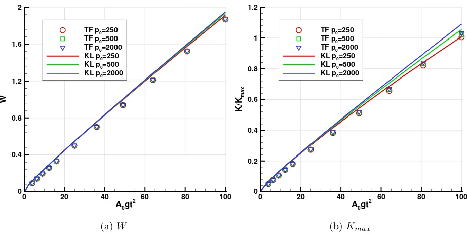
Calculations using both models have been performed for different initial pressures at the interface (p0=250, 500, 2000 dyn/cm2) in order to assess the incompressibility limit of the
A0gt2
W
0 20 40 60 80 100
0 0.4 0.8 1.2 1.6 2
TF p0=250 TF p0=500 TF p0=2000 KL p0=250 KL p0=500 KL p0=2000
(a)W
A0gt2
K
/K
m
a
x
0 20 40 60 80 100
0 0.2 0.4 0.6 0.8 1 1.2
TF p0=250
TF p0=500
TF p0=2000
KL p0=250
KL p0=500
KL p0=2000
(b)Kmax
FIG. 7: Time evolution of mixing width and maximum turbulent kinetic energy for RTI mixing of fluids with initial density ratio 3:1. Different initial interface pressures.
the larger value of W with increasing initial interface pressure is also linked to the higher
Kmax, thus resulting in a larger turbulent viscosity µt and mass-fraction diffusion. Though
the final value (t = 10, A0gt2 = 100) for Kmax also increases with higher initial interface
pressure in the TF model, it is more pronounced in the case of the K-L model.
Figures 8aand 8b show the V F and K/Kmax profiles, respectively, at two time instants
for the RT case with density ratio 3:1 and initial interface pressure p = 500 dyn/cm2.
Comparisons are also presented with ILES [9]. The (3D) ILES results (t = 10 sec.) have been spatially averaged to allow comparisons with the 1D turbulence model calculations. The Kmax and W profiles show that both turbulence models achieve self similar solutions. The V F profiles are almost identical and in excellent agreement with ILES. Some minor discrepancies appear in theK/Kmax profiles, especially on the spike side, where the TF and
K-L results agree closely.
2. Grid Convergence study
[image:30.612.76.537.78.309.2]X/W
V
F
-4 -2 0 2 4
0 0.2 0.4 0.6 0.8
1 ILES
TF t=6 TF t=10 KL t=6 KL t=10
(a)V F vsX/W
X/W
K
/K
m
a
x
-4 -2 0 2 4
0 0.2 0.4 0.6 0.8
1 ILES
TF t=6 TF t=10 KL t=6 KL t=10
(b)K/Kmax vsX/W
FIG. 8: Volume fraction(a)and Turbulent kinetic energy(b)profiles for RTI mixing of fluids with initial density ratio 3:1.
convergence study has been carried out using three grids with Nx = 100, 200 and 400 cells, respectively.
The reduction in numerical dissipation associated with the cell size (filter) is apparent only at the early stages of the simulation, until the turbulent viscosity of the model becomes large enough to have a greater effect on the results than the numerical dissipation of the convection terms. This is shown in the integral mixing width (W) and maximum turbulent kinetic energy (Kmax) results in Figures 9-10. The grid resolution seems to have an effect
on the growth rate only at the early stage of the simulation. Once the turbulence viscosity becomes sufficiently large, all grids achieve a similar growth rate. This is further supported by the negligible differences in the profiles of K/Kmax and W, for both the K−L and TF
models, shown in Figures 10a and 10b.
For the K −L model the reduction in numerical dissipation due to the increasing grid resolution occurs primarily at the beginning of the simulations, during which there is a noticeable gradual divergence of the mixing width (W) and maximum turbulent kinetic energy (Kmax) growth rates up until the turbulence model diffusion becomes the leading
A0gt2
W
0 20 40 60 80 100
0 0.4 0.8 1.2 1.6 2
TF Nx=100
TF Nx=200
TF Nx=400 KL Nx=100
KL Nx=200
KL Nx=400
(a)W
A0gt2
K
/K
m
a
x
0 20 40 60 80 100
0 0.2 0.4 0.6 0.8 1 1.2
TF Nx=100
TF Nx=200
TF Nx=400 KL Nx=100
KL Nx=200
KL Nx=400
(b)Kmax
FIG. 9: Time evolution of mixing width and maximum turbulent kinetic energy for RTI mixing of fluids with initial density ratio 3:1. Effect of grid resolution.
mixing width shows little variation with mesh. As already noted, the initial conditions
model is used to minimize this variation. For K/Kmax there are also small ”delays” due to
the change in mesh size. For both the K−L and TF models the effect of mesh size for this simple test is small and not significant for practical applications.
D. Density Ratio 20:1
Several calculations were performed for different interface pressures and specific heat capacity ratios. A summary of the test cases are presented in Table IV.
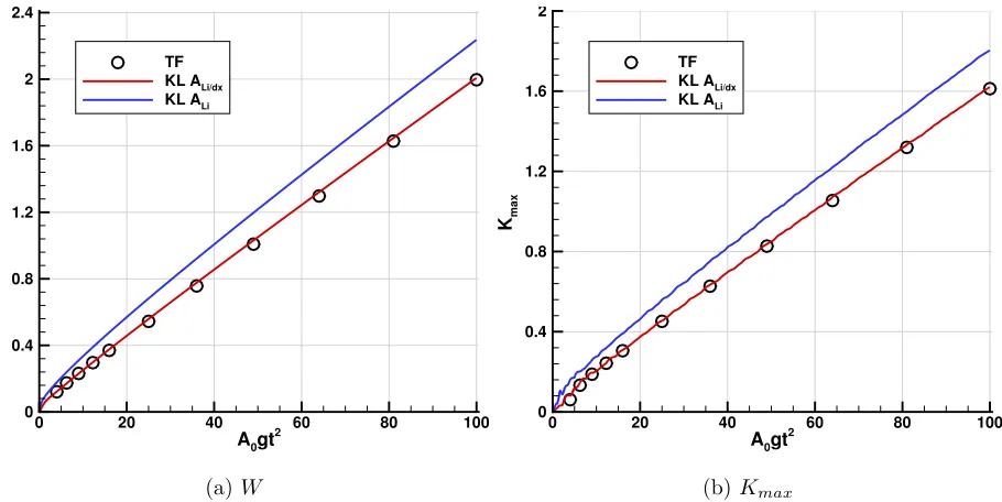
In addition to investigating the TF and K-L models behavior for different interfacial pressures and specific heat capacity ratios, we have performed a series of tests for the K-L models to examine the effects of: i) turbulent diffusion of internal energy term (section
III E), i.e., comparing the results obtained using equation (17) (internal energy diffusion) to those of equation (62) (enthalpy diffusion); and ii) calculation of the local Atwood number (Section III F), using equations (37)-(43) or (44)-(47).
Comparison of the results for the late time growth rate parameters of W and Kmax
X/W
V
F
-4 -2 0 2 4
0 0.2 0.4 0.6 0.8 1
ILES
TF Nx=100
TF Nx=200
TF Nx=400
KL Nx=100
KL N
x=200
KL Nx=400
(a)V F vsX/W
X/W
K
/K
m
a
x
-4 -2 0 2 4
0 0.2 0.4 0.6 0.8 1
ILES TF Nx=100 TF N
x=200 TF Nx=400 KL N
x=100 KL Nx=200 KL Nx=400
(b)K/KmaxvsX/W
Case p0 (dyn/cm2) γ1 γ2
1 1000 5/3 5/3
2 2000 5/3 5/3
3 4000 5/3 5/3
4 1000 2 2
5 1000 4 5/3
TABLE IV: Simulations carried out for density ratio 20:1
Case W Kmax
ILES 0.019254 0.0170 TF 0.019410 0.015407 K-L 0.018964 0.015157
TABLE V: Self-similar growth rateparameters of W and Kmax
for density ratio 20:1;p0= 2000 dyn/cm3 and γ1 =γ2=5/3
Both turbulence models are in fairly good agreement with ILES, however the TF model provides overall better results.
1. Effect of initial interface pressure
Calculations have been performed for fluids of an initial density ratio 20:1 and equal specific heat capacity ratios γ1 = γ2 = 5/3. The parameter altered is the initial interface
pressure, rangingp0=1000, 2000 and 4000 dyn/cm2, in order to assess the incompressibility
limit of the turbulence models. Self-similarity is achieved (Figure11) by both models while the change in the initial interface pressure has almost negligible effect in either model.
The VF and K/Kmax results at different time instants and for initial interface pressure
of p = 4000 dyn/cm2 (Case 3) are shown in Figures 12a and 12b, respectively. Similar to
the 3:1 density ratio, the V F results are nearly identical and in very good agreement with ILES. Furthermore, the TF and K-L results for K/Kmax are in very good agreement with