1
Autonomous Swarm Testbed with Multiple Quadcopters
Ruaridh Clark
1, Giuliano Punzo
1, Gordon Dobie
2, Rahul Summan
2,
Charles Macleod
2, Gareth Pierce
2and Malcolm Macdonald
11
Advanced Space Concepts Laboratory, Department of Mechanical and Aerospace Engineering, University of Strathclyde, Glasgow, United Kingdom.
2
Department of Electronic and Electrical Engineering, University of Strathclyde, Glasgow, United Kingdom.
Abstract: A testbed has been developed to validate and trial swarm engineering concepts. The vehicles used in this testbed are commercially available Parrot AR.Drone quadcopters that are controlled through a computer interface connected over a 65 Mbps, IEEE 802.11n (Wi-Fi), network. The testbed architecture is presented with the implementation of a distributed controller, for each vehicle, discussed. The controller relies on a tracking system to provide precise information on the position and orientation of the aerial vehicles within the enclosure. This enables the autonomous and distributed elements of the control scheme to be retained, whilst alleviating the drones of the control algorithm's computational load. The testbed is used to control 3 drones effectively, where the control, communication and tracking systems are scalable to at least 12 drones. The paper also introduces the application of swarm engineering in remote visual inspection, with multiple airborne platforms visually inspecting a target by completing coverage bands before transitioning to another height. A kinematic field enables the drones to follow this path autonomously with the field being asymmetrically modified as a result of drone interactions. This modification of the field for a single drone is shown to prevent vehicle collisions by enabling queuing behind the leader. Using a swarm of 3 quadcopters, the coverage time for a target can be reduced by around 60% when compared with a solitary drone. Finally the three-dimensional model of a target that is generated from drone footage is presented; this surface-meshed model is constructed in post-processing, through photogrammetric analysis of the collected images.
Key words:
Autonomous, Inspection, Quadcopter, Swarm, Testbed
.
I. INTRODUCTION
2
increasing the technology readiness level (TRL) of autonomous systems rather than individual drone performance.
II. TESTBED ARCHITECTURE
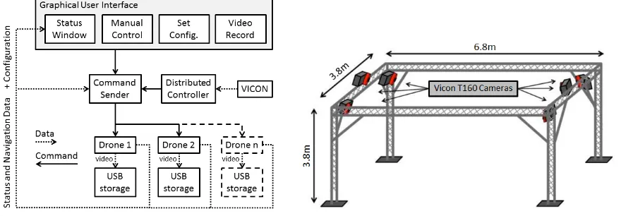
The aerial vehicles used are commercially available quadcopters, Parrot AR.Drones, that carry a 720p HD camera and have a 10 12 minute flight time using a Lithium-Ion Polymer (1,000 mAh) battery. The quadcopters are around 50 cm in length and controlled through a computer interface connected over a 65 Mbps, IEEE 802.11n (Wi-Fi), network. They are capable of transmitting information about their status and configuration, including battery charge, control state (landed, flying etc.), as well as attitude and speed estimation. Video is recorded onto a USB memory storage device on-board the quadcopter that can be removed and the footage viewed after landing.
The quadcopters are tracked from above by 6 Vicon T160 positioning cameras, as displayed in Fig. 1 (b), providing 6 degree of freedom information for an estimated error of less than 3 mm throughout the volume[4]. The cameras identify the individual quadcopters by detecting infrared light reflected from a unique pattern of spherical (14mm diameter) markers affixed to the vehicle’s frame. Positional
information is passed over the wireless networkat 100 Hz to the computer that implements a distributed controller for each vehicle. The control scheme is centralised to one computer, allowing it to maintain its autonomous and distributed elements whilst alleviating the quadcopters of the control algorithm’s computational load.
Open source code, developed in C#[5], to control a solitary Parrot AR.Drone was adapted to command multiple drones through a Graphical User Interface (GUI). The software architecture is depicted in Fig. 1 (a); programme capabilities include autonomous and manual control of the drones while displaying the status and navigation data through the GUI. In this work, a maximum of three drones are used, but the architecture is designed to accommodate larger groups of drones. Fig. 1 (a) shows that the distributed controller and GUI have their command outputs processed by the Command Sender before
[image:2.595.79.519.564.717.2]3
being passed onto the drones. This allows manual commands to be passed to the drones while in autonomous flight, allowing for example the initiation of video recording or escape from autonomous mode into manual flight control. The Command Sender passes on commands at 30 Hz, as recommended in the Parrot developer guide[6], to ensure smooth flight.
The commands, including yaw rate, vertical velocity, pitch and roll angle, are transformed to 32-bit integers according to the IEEE754 standard before being transformed to an ASCII string and passed on to the vehicle control software through a User Datagram Protocol (UDP) port.
Turbulence Disturbance
The volume of the testbed is the main restriction on the number of drones used and the manoeuvres that can be conducted, but a less obvious aspect of this constraint is the influence of turbulence on quadcopter performance.
The Parrot Ar.Drones comes with two protective Styrofoam cover options; a minimal shell for outdoor flight and an indoor cover protecting the blades from collisions. By using the outdoor shell the disturbance effect is reduced but still evident when flying three drones in the volume. For a drone commanded to hold its position, when three drones are being controlled and two of them are held at the extremities of the volume, there is a root-mean-square error (RMSE) of approximately 4cm for the x and y position in the global reference frame. However, when three drones are flying unrestricted in the volume this error increases to lie in the range of 10 20 cm.
Network Capacity
A 65Mbps wireless connection is used to communicate with the quadcopters and the computer performing the Vicon marker tracking. When controlling three drones, in normal operation mode, the network usage is at 16% (4% per drone + 4% for Vicon positional data). At this data transfer rate, communication latency becomes notable. A ping test performed at this network usage results in delays of 30 80 ms when communicating with a drone.
To reduce the latency, the quadcopters’ status was set to the lower transmission rate of 15Hz, instead of the default of 200Hz. In this mode the network usage drops to just over 5.2% ( 0.4% per drone). The ping test now returning delays in region of 1 4 ms with growth in this latency not occurring until network usage reaches just under 10%. Therefore, given a larger physical volume the system should be able to accommodate at least 12 drones before any increase in communication latency occurs.
III. GUIDANCE AND CONTROL
4 x, y Positions and attitudes
: : : :
On-board control software Linear controller Global to local reference frameϑ,φ,vz,𝜓 (Vx, Vy, Vz)B
(Vx, Vy,)G
ψ (Vz)G
Proportional controller Kinematic field z,ΨG On-board control software Linear controller Global to local reference frame
ϑ,φ,vz,𝜓 (V
x, Vy, Vz)B (V
x, Vy,)G
ψ (Vz)G
Proportional controller Kinematic field z,ΨG x, y
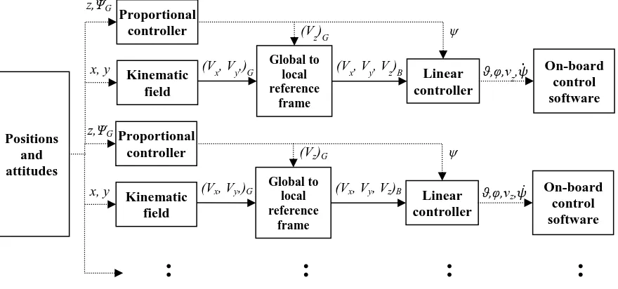
architecture is illustrated in Fig. 2 where the guidance block is provided with the drone’s own position and the relative positions of the other drones in the field. Based on this information the local kinematic field of each drone is computed; producing the desired velocities in the horizontal plane of the external reference frame. These are passed to a linear controller that provides the pitch and roll angles to the on-board controller with desired yaw and vertical speeds also supplied. This in turn commands the motors to execute the requested manoeuvre. The specifics of this control scheme are detailed in the following paragraphs.
Kinematic field definition
The kinematic field is defined in the horizontal plane as the target is assumed to have central symmetry characteristics. However, nothing prevents the definition of three-dimensional velocity fields to accommodate more complex geometries.
The fundamental structure of the field is a modified version of the Hopf bifurcation function used by Bennet and McInnes[7] and described as
2 2
1
(
x) Rx
dx
v
c
x
y
(1)2 2
1
( x
y) Ry
dy
v
c
x
y
(2) [image:4.595.78.518.492.698.2]where, R is the radius of an ideal circular trajectory in the horizontal plane enclosing a central target, c1 is a constant and μ is a scalar parameter that, taken positive, guarantees the emergence of a limit cycle in the field.
5 In particular, the choice of
2
1
c
R
(3)guarantees a circular trajectory of radius R around the centre. This can be easily verified by transforming eqs. (1) and (2) into polar coordinates and checking that the radial velocity is always null at a distance R from the centre. It can also be easily verified that, along the trajectory, the tangential velocity is constant.
The kinematic field is completed by a function that provides a more robust control system by strengthening the control action close to the target to avoid collisions, while effectively leaving the characteristics of the field produced with eqs. (1) and (2) unaltered. This function is a radial field in the form 1 / (1R), which increases the repulsion from the centre while decreasing the attraction at large distances, thus making approaching manoeuvres smoother and preventing overshoots in the direction of the target. The resulting field is described by
21 2 2 2
1
x
d M xc
v
c y
Rx
y
x
y
x
(4)2 2
1
2 2
c
( x
) Ry
1
d M yc
y
x
x
y
y
v
(5)where cm is a constant used to scale the whole expression as appropriate to fit its output within the control architecture. The values of the constants introduced so far are 7
1.5 10
m
c x , 5
1 3 10
c x and 1200
R . In Fig. 3 this field is represented with arrows and eight streamlines joining in the limit cycle.
Collision Avoidance
A popular way to perform collision avoidance in multi-agent systems is through mutual repulsive potential, see for example ref. [7 – 10]. This way each agent alters the kinematic field by producing a short-range repulsive action on the other agents. This is an efficient but crude mechanism for performing collision avoidance; therefore a less disruptive approach was used that blends well with the global kinematic field. This new approach acts like an asymmetric repulsive function by modifying the kinematic field for one drone approaching another, initially reducing the magnitude of the field’s rotating component. In order to be effective, only the trailing drone is inhibited. Identification of this drone is achieved by considering the scalar product of the relative position vector with the desired velocity vector. In reference to Fig. 5 a binary variable, h, is defined on the basis of the scalar product with
1 2 1 0 1
des P
V h (6)
1 2 1 0 0
des P
6
where P2 1 is the position vector of drone 2 with respect to drone 1 in the global reference frame. This
enables the kinematic field to be modified asymmetrically, i.e., only the trailing drone, where h1, is affected.
The desired velocity of drone 1, as calculated in eqs. (4) and (5), is filtered to create the asymmetrically modified kinematic field. This is achieved by replacing the constant c1 with the following function
2 *
1 ( 1) 1
c H P c (8)
where H(P2 1) scales the rotational component of the field as a function of P2 1 , Vxd*and d*
y
V are the desired x and y velocity vectors for drone 1 within the modified field. This changes does not affect the radial velocity at distance R from the target centre, which remains null, as the calculation of
, shown in eq. (3), is updated to2
* 1
R
c
(9)This asymmetrically modified field only occurs when drones are within close proximity. The 2 1
(| P |)
H term that governs this proximity enables a threshold distance to be defined, whereby passing this point results in a switch of direction for the rotational component of the kinematic field, as depicted in Fig. 5. The modified field, therefore, enables station keeping at the defined distance from the target until the leading drone moves on. The function used is in the form
2 2 1
(|P | )
2 1 2 1
2 1
2 1 2 1
| P
|
| P
|
(| P
|)
|| P
|
|
|
| P
||
i
c
H
e
[image:6.595.107.491.93.299.2]
(10) [image:6.595.103.285.98.264.2]Fig. 3:Arrow plots and streamlines for the kinematic field with R = 1200 mm.
7
[image:7.595.110.500.87.241.2]
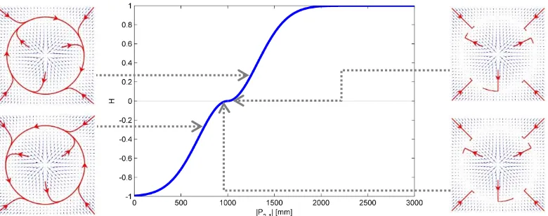
Fig. 5:Centre plot: (| |) according to eq. (10) with ρ = 1000 and ci = . Left and right plots:
Modified kinematic field (displayed with arrow plots and streamlines) for varying values of .
where
defines the threshold distance between drones and ci is a scaling factor that influences the gradient of the function.Fig. 5 shows how the scaling of the kinematic field’s rotational component affects the modified field. This figure highlights that H equals 0 at the threshold distance of 1m (1000), with the rotational component of the kinematic field acting in opposite directions either side of this distance.
In Fig. 6 the three quadcopters are controlled using the kinematic field, described previously, with all drones pointing at and circling around a central target. When implementing this control for more than two quadcopters, a drone will only consider the closest drone ahead of it when modifying its kinematic field.
Altitude Control
[image:7.595.79.510.609.739.2]A proportional controller is implemented to control the altitude of the drones in the volume, which operates in unison with the quadcopter’s on-board, ultrasound dependant, altitude controller. The output of the proportional controller is converted from the global to the body reference frame as shown in Fig. 2. Waypoints were used in conjunction with this controller to switch between coverage bands at different heights, which was required for the case study discussed in the following section.
Fig. 6: Sequence of images (6 second intervals) showing the asymmetrically modified kinematic field in action for 3 quadcopters.
1
1
1 2
2
2 3
3
8 Attitude Control
In a typical quadcopter, pitch and roll angles are coupled with the forward and lateral motion respectively. The design enables forward or side force components to be produced by tilting the drone. When no forward or side movements are commanded, the vehicle hovers and in this phase the attitude is controlled in closed loop by the on-board controller only. This is overridden by the remote controller when controlling the yaw angle, which is controlled in the same closed loop manner as the altitude. For the inspection task, discussed in the following case study, the attitude controller keeps the drone’s x axis pointing in the direction of the target whilst the quadcopter manoeuvres around it. As a consequence, the desired azimuth changes with time. This is defined as
1 _
tan
i des i iy
x
(11)where xi and yi are the coordinates of the vehicle in the global reference frame, with the ± sign used to select the smallest angle possible. The error is then mapped to an angular rate through the linear controller.
Linear Controller
The linear controller maps the desired velocity of each drone to commanded pitch and roll angles. The desired velocity vector is decomposed along its forward and lateral components in the body reference frame and these are scaled by a proportional controller. The result is then filtered to output in the range
] 1,1[ , required for the AR.Drone on-board software, by using the hyperbolic tangent function
*
tanh( )
(12)where
is the vector of the controlled variables (including the roll angle
, pitch angle , vertical velocity Vz and yaw rate
) and * is the normalised output.For the purpose of this paper a simple proportional controller is used to map from desired forward and lateral velocities according to the kinematic field, vertical velocity and azimuth angle to commanded pitch and roll angles, vertical velocity and yaw rate. The controller is expressed by
_ y_
(z
z)
(
)
x des des z des r desk
k
k
k
(13)where, x des_ and y_des are the forward and lateral velocities in the body reference frame produced by the kinematic field, des is the desired azimuth angle that varies with time, is the actual one, and
k, k, kz, k are the gains of the proportional controller. The values of the gains used here are
0.7
9
IV. CASE STUDY:3DMODEL GENERATION USING AN AIRBORNE QUADCOPTER SWARM
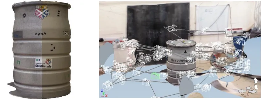
Remote inspection is a potential application for the airborne swarm, which could be deployed to monitor structures especially those in human-hazardous or inaccessible environments. Therefore a case study was conducted in the testbed environment, detailed previously, with the goal being to gather footage of a central target and convert those images into a 3D Computer Aided Design (CAD) model. The swarm provides complete and rapid coverage of the object of interest, which in this case was an intermediate level, nuclear waste storage drum.
Using the kinematic field described previously the drones were able to examine the entire circumference of the drum by always pointing towards its centre, before moving on to a different section and continuing the inspection. Each drone, therefore, recorded video of the target with the images first collated, before being processed by Autodesk’s 123D Catch[11] to create the 3D models shown in Fig. 7. This software uses photogrammetric analysis to process the images, where common features are identified and images stitched together to provide an estimate of target geometry. Automated feature matching was facilitated by the manual selection of common points appearing in at least three images. This process ensured that images were stitched in the correct location and common features were found, which was difficult in this case given the monochromatic and symmetrical nature of the drum. The final result is displayed side-by-side with a photo of the drum in Fig. 7 (a). The model contains most of the drum’s features but had difficulty in areas of poor coverage, primarily the lid and the base of the drum.
Inspection could be conducted with one drone, but multiple drones provide faster coverage while offering some redundancy in the system when considering the possibility of individual drone failure. To compare the coverage speeds, when using different swarm sizes, a flight time was recorded for filming four coverage bands. The drones were required to have collectively achieved complete coverage around the circumference before transitioning to another band 30 cm below. For 1 drone this took around 160 s, this time decreased to around 65% (104 s) of that period for 2 drones and then was reduced to around
[image:9.595.84.507.579.740.2]40% ( 64 s) in the 3 drone case.
10 V. CONCLUSION
A testbed that relies on a Vicon tracking system and wireless network connection to control multiple Parrot Ar.Drones has been presented. The performance of a 3 drone swarm has been evaluated, with the coverage time being about 60% less than in the single drone case, and the potential identified for scaling the system up to 12 drones. When considering these larger swarms, intelligent collision avoidance becomes even more critical. The avoidance mechanism used is effective in controlling 3 drones. Crucially, it provides a more reliable and verifiable response than that of mutual repulsive interactions where drones are repelled from each other with no reference to the global kinematic field. Both the collision avoidance and kinematic field control scheme are robust being based on smooth mathematical functions, which operated successfully in turbulent conditions that were detrimental to flight control. The RMSE in positional control reaching 20cm in turbulence, with three quadcopters flying in the volume, compared with the 4cm error recorded in a reduced turbulence flight.
The overarching goal of the testbed is to raise the TRL of swarm based systems. A remote inspection case study conducted in the testbed has confirmed the feasibility of generating a 3D model from in-flight footage. Improvements can still be made in the model generation process, to increase accuracy and automation, but the system is now in a position to be progressed to a ‘real-world’ demonstration.
VI. REFERENCES
[1] Michael N, Mellinger D, Lindsey Q and Kumar V. (2010) The GRASP multiple micro-UAV testbed.
Robotics & Automation Magazine. IEEE. 17(3): 56-65.
[2] Vicon motion tracking system, http://www.vicon.com/Software/Tracker.
[3] Sanchez-Lopez JL, Pestana J, de la Puente P and Campoy P. (2013) Visual quadrotor swarm for IMAV 2013 indoor competition. Internationcal Micro Air Vehicle Conference and Flight Competition. Toulouse, France.
[4] Dobie G, Summan R, MacLeod C and Pierce SG. (2013) Visual odometry and image mosaicing for NDE.
NDT and E International. 57: 17-25.
[5] Balanukhin R. (2013) AR.Drone [Source code], https://github.com/Ruslan-B/AR.Drone.
[6] Piskorski S, Brulez N, Eline P and D’Haeyer F. (2012) AR.Drone developer guide SDK 2.0, Parrot. [7] Bennet DJ and CR McInnes. (2009) Verifiable control of a swarm of unmanned aerial vehicles.
Proceedings of the Institution of Mechanical Engineers, Part G: Journal of Aerospace Engineering. 223(7): 939-953.
[8] Badawy A and McInnes CR. (2009) Small spacecraft formation-flying using potential functions. Acta Astronautica. 65(11-12): 1783-1788.
[9] D’Orsogna MR, Chuang YL,Bertozzi AL and Chayes LS. (2006) Self-propelled particles with soft-core interactions: Patterns, stability, and collapse.Physical Review Letters. 96(10): 104302.
[10] Leonard NE and Fiorelli E. (2001) Virtual leaders, artificial potentials and coordinated control of groups.