Developments in high fidelity surface force models and their relative effects on orbit prediction

Developments in High Fidel

ity Surface Force Modelling and

their Relative Effects on Orbit Prediction

Dr Stuart Grey1 _{and Prof Marek Ziebart.}2

University College London, London, United Kingdom, WC1E 6BT

This paper presents developments to a set of high fidelity spacecraft surface force models. These models address the problem of errors in orbital prediction and orbital determination due to un-modeled and under-modeled surface forces on spacecraft. These models have been validated individually but in this paper the most recently developed models are applied together to give an insight into how they effect a spacecraft in orbit. A significant reduction in error between the predicted orbit and tracking data is shown when all the models are implemented.

Nomenclature

Fnormal = force normal to surface

E = incident flux

A = area

c = speed of light in a vacuum (299792458 ms-1₎

θ = angle of incidence ν = absorptivity in SRP µ = reflectivity

Fshear = force along surface

Tf = temperature at front of solar panel Tb = temperature at back of solar panel Rtotal = effective resistance of total panel

εf = emissivity at front of solar panel

εb = emissivity at back of solar panel

σ = Stephan-Boltzmann constant (5.6699 x10-8 Wm-2K-4)

qelec = current drawn from panel

α = absorptivity in TRR

aTRR_SP = acceleration due to TRR on solar panels

aTRR_MLI = acceleration due to TRR on the MLI on the spacecraft bus m = mass of spacecraft

fs = flux arriving the spacecraft from each grid cell IT = total intensity at grid cell

rs = distance to spacecraft

I.

Introduction

recise orbit determination (POD) and orbit prediction of spacecraft plays a key role in a diverse range of space missions. Spacecraft surface forces, while orders of magnitude smaller than gravitational forces are central to the accurate determination and propagation of spacecraft orbits. The past decade has seen the rapid development and adoption of more complex surface force models. This paper will outline an approach to modelling four of these surface forces and their effects. The forces that will be discussed are Solar Radiation Pressure (SRP), Thermal

1 _{Lecturer in Space Geodesy, Department of Civil, Environmental and Geomatic Engineering, Chadwick Building,} Gower Street, London, WC1E 6BT, AIAA Member.

2 _{Professor in Space Geodesy, Department of Civil, Environmental and Geomatic Engineering, Chadwick Building,} 2 _{Professor in Space Geodesy, Department of Civil, Environmental and Geomatic Engineering, Chadwick Building,} Gower Street, London, WC1E 6BT, AIAA Member.

Radiation (TRR), Earth Radiation Pressure (ERP) and Antenna Thrust (AT). The magnitude of these forces varies with orbital regime and spacecraft. For instance ERP becomes much more significant at low earth orbit (LEO) altitudes but should not be ignored at higher orbits if precision is required. These surface forces are also greatly dependent on the spacecraft structure and spacecraft surface material properties. The approach developed and refined at University College London (UCL) is to model the spacecraft to a very high level of detail and use accurate values for the reflectivity, absorbtivity, emissivity etc of the surface. Fundamental physical principles are used to model the interaction between the spacecraft environment and the spacecraft structure. This paper aims to share insights into the calculation of the surface forces on spacecraft and provide a catalyst for applying high fidelity surface force models to a wider range of space missions.

II.

Solar radiation Pressure (SRP)

SRP is the force exerted on a spacecraft's surface due to collision with photons originating from the sun. Einstein’s Special Theory of Relativity describes the relationship between the energy of a photon and its momentum and when a photon strikes a spacecraft there is a momentum exchange. The amount of momentum transferred to the spacecraft is dependent on the energy of the photon and whether it is absorbed or reflected by the spacecraft. From this starting point a relationship can be developed for the force per unit area at 1 astronomical unit from the sun.

With this knowledge we can then adopt one of two broad approaches to modelling the SRP effects on a spacecraft, either an empirical approach or an analytical approach. In the empirical approach a model is formulated with a number of coefficients that determine its response to an incident solar flux. These coefficients are then estimated by analysing orbital tracking data over a certain period time to provide a model of how the SRP may have effected the spacecraft. A key benefit of the empirical approach is that it requires no specific knowledge of the spacecraft (although a simplified model, such as a box and wing model, may be used). The disadvantage of this approach is that we cannot know that the variation in the SRP model coefficients is purely down to the effect of the incident photon pressure as other effects that occur over similar time scales will be aliased into them. The empirical approach allows for the determination of very precise orbits but does not allow us to isolate the many forces that act on a spacecraft which is needed for long term orbit prediction1.

In the analytical approach the SRP effect is determined by using as much information about the spacecraft as possible along with models of the physical interaction between the incident flux and spacecraft. An analytical model provides the ability to model the forces due to SRP without any spacecraft tracking data at the expense of a significantly more complicated modelling and calculation process. This lack of reliance on tracking data makes approaches which are more analytical in nature much more suitable for long-term orbit prediction. More accurate a priori models also help to reduce aliasing of SRP into other parameters, essentially removing a level of uncertainty about a forces source.

In reality there are a range of approaches between these two extremes and both empirical and analytical approaches are used depending on the specific orbit prediction or orbit determination problem. In a typical empirical approach the spacecraft is modelled using a cannonball or box and wing approximate spacecraft model. The acceleration due to incident flux on these primitives can be computed quickly and the parameters of the physical model solved for during the orbit determination process. These models though cannot account for all of the spacecraft geometry and material properties.

In the UCL analytical approach2 _{a ray tracing technique is used on a complete model of the spacecraft. This} involves calculating how incident light intersects the spacecraft geometry and the resultant force when it does. The model also allows for secondary intersection due to reflection and fully models spacecraft self-shadowing.

A. Ray tracing approach

Ray tracing as a technique is very simple in theory3. The interaction between an incoming flux and a structure is calculated by splitting the flux into may small component parts, or rays, calculating the interaction for each ray then summing the contribution from each ray to arrive at a value for the system as whole.

number of elements that make up the spacecraft. Because of this it is usual to try and keep the number of triangles used in the description of the geometry to a minimum while still describing the structure as well as possible. The decomposition of complex shapes into a number of triangles to aid computation is called tessellation. An alternative approach is instead of tessellation to describe each element using geometrical primitives such as cylinders, discs, parabaloids and n-sided polygons where appropriate..

This geometrical primitive approach requires a significantly more complicated ray intersection test but reduces the number of parts that make up the spacecraft. The key benefit however is that by using geometrical primitive the exact intersection point, surface normal etc. can be calculated rather than that of the triangulated approximation. This greatly helps with the problem of trying to model how incident light is reflected from the spacecraft’s surface.

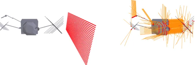
The ray tracing part of the modelling process starts with a grid of ray starting locations being defined on a plane orthogonal to the incident radiation flux direction. Each of these rays are then taken in turn and its path is determined as it enters the modelling space from the flux source direction. This ray is then tested against each geometrical components in the spacecraft micro-model to see if there are any intersections. These intersections are then ordered by distance from the ray source and the intersection with the minum distance to the flux source taken as the true intersection. Once the intersection has been found vectors normal to the surface of the spacecraft and in the shear force direction at the interesection point can be calculated. The area used for the calculation is determined from the spacing between the rays. This means of course that using more rays will give a more complete picture of how the photons interact with the spaceraft.

The force normal to the surface due to a radiative flux is dependent on the surface reflectivity and absorbtivity and can be described using the following equation4_.

Fnormal=−

EA

c cosθ (1+νµ)cosθ+

2 3

" #

$ %

& 'ν(1−µ)

" #

$ %

&

' (1)

The force in the shear direction due to a radiative flux is:

Fshear= EA

c cosθsinθ(1−vµ)

(2)

Depending on the surface proporties of the material some proportion of the light may be reflected. This reflection can be a combination of both diffuse and specular reflection. In the case of the diffuse component a lambert distibution is used and no new rays are created. In the case of the purely specular componet of the reflection a new ray is created at the intersection point and propagated again to find any secondary interesection points. Its energy is reduced by any absorbtion at the first reflection point.

This process is repeated for each ray in the grid and then the forces from each ray, in the spacecaft body frame are summed to give a total force in the body frame for that incident radiation direction. This process is then repeated from a range of directions around the spacecraft. For certain spaceraft with well known and reliable attitude control laws the direction is constrained to some arc in the spacecraft body frame (with some allowance for error). In this case the directions chosen for the SRP response model are placed along this arc or adjacent to it. For spaceraft with a

greater variation of attitude or spacecraft with no attitude control the incident radaition dirction is varied across the entire spacecraft frame in order to give good coverage, whatever the incident direction in reality.

The flux model for SRP is relatively simple. The flux is defined as 1361Wm2 _{at 1au and is simply scaled for} distance. The solar flux must also be scaled when travlleing through the penumbral region and a number of appraches may be used5,6_{. The force due to SRP is typically larger that the other three forces outlined in this paper} but modelling SRP alone is not sufficient for many POD tasks as shown in the validation section.

III.

Thermal Re-Radiation (TRR) modelling

TRR modelling utilises the same spacecraft model and material properties and calculates the thermal response of the material to the incident radiation flux and the resultant emission of thermal photons. This is then used to calculate the resultant force on the spacecraft.

The process of modelling the force due to TRR has two main components7_{, determining the temperature of the} surface of the spacecraft and then determining the force exerted by the emitted thermal photons across the entire surface of the spacecraft. In the UCL approach to thermal modelling the precise spacecraft structural model that was developed for the SRP calculations is reused.

In order to determine the temperature of the surface of the spacecraft we need to know which areas are illuminated and the reflectivity/absorbtivity of the materials of the individual parts of the spacecraft. Using the data from the SRP computation we have a very good model of which areas are illuminated, just by collecting the intersection points from the ray-tracing step.

B. Temperature of solar panels

The more complex step is to model the temperature of the surface due to this incident radiation. A simpler subset of the problem is to calculate the temperature on the surfaces of the solar panels. Any SRP or TRR effects on the solar panels will dominate effects on the bus due to the difference in surface area for most spacecraft. If the solar panel is treated as a plate with two emitting faces, front and back, then an energy balance equation based on the energy incident on the front of the panel, the energy transmitted through the panel and the energy emitted from the front and the back of the panel can be devised7_.

The temperature at the back of the solar panel can be calculated using the following equation: Tf =−Tb+RtotalεσAT

4

b (3)

The temperature at the front of the panel is found by substituting in the temperature at the back of the panel from the previous equation into this equation:

αWcosθ=εσ(Tb+RtotalεσATb 4

)4 +εσTb

4

+qelec (4)

The temperature at the front and the back of the panel is computed numerically using the newton-raphson method. Once these temperatures have been determined the acceleration can be calculated as:

aTRR_SP=

2Aσ(εfTf 4

−εbTb 4

) 3mc

(5)

C. Temperature of multi-layered insulation (MLI)

TMLI

4

=αWcosθ+εeffσTsc

4

σ(εMLI+εeff)

(6)

The value for the temperature of the internal of the spacecraft can be substituted into equation 6 above to determine the temperature of the MLI which the yields the following equation for the acceleration due to TRR on from the MLI:

aTRR_MLI =

2ApσεMLITMLI

4

3mc

(7)

D. Summary of TRR Calculations

To summarise, the UCL approach to modelling TRR uses two models, one for the thermal equilibrium of the solar panels and one for the thermal equilibrium of the MLI covering the bus. For the solar panels the incidence angle of the solar flux is calculated and the thermal equilibrium temperatures calculated for the entire area of the solar panels. The amount of thermal energy emitted by the front and the back of the solar panels is then calculated in order to find the resultant acceleration.

For the spacecraft bus a ray-tracing technique is used to calculate which areas of the spacecraft are illuminated. Then, for each ray intersection area a thermal equilibrium is calculated and TRR force computed. In a similar manner to the SRP calculation the TRR values for each ray are then summed to calculate the acceleration on the bus as a whole.

IV.

Earth Radiation Pressure (ERP)

The ERP model again uses the photon-spacecraft interaction model used by the SRP model. The difference is that instead of a solar flux, a flux is computed that incorporates the fluxes both emitted from and reflected by the Earth. These fluxes are based on the CERES mission earth radiation fluxes9_{. The CERES data is based on a} 2.5°x2.5° grid and the data used in calculating the ERP fluxes are the monthly total-sky averages of both long wave

and shortwave fluxes.

The flux radiated by each cell at a given time is calculated by combining the long wave and shortwave CERES fluxes depending on the direction of the Sun in relation to the Earth.

The visibility of each of these grid cells is determined by checking that the angle between the surface normal in the centre of the grid cell and the satellite-grid vector is less than 90°. This gives us a set of grid cells that are

visible.

The flux from each of these cells is then scaled for viewing angle by assuming a lambert distribution of flux from the cell and then scaled for distance to the spacecraft. Care must be taken to remember that these grid cells are

Figure 2. The flux emitted by the Earth due to long wave emission (the entire surface) and short wave reflection (the day side, in this case the right hand side of the figure).

not at the surface of the earth but at 30km altitude. Figure 3 shows the areas of the Earth’s surface visible to Envisat and a representative GPS satellite over a single orbit. Figure 4 shows the amount of flux reaching the spacecraft at a single epoch and Figure 5 shows how this varies over a typical orbit. The flux at the spaceraft from each cell can be calculated as follows10_:

fs=

ITdAcosθ

πr2 (8)

The interaction between the flux and the spacecraft is calculated using the same methods used in the SRP calculation. Exactly the same spacecraft model is used and only the incident flux changed. The flux is treated at this stage as purely radial. Example fluxes are given for both Envisat and a representative GPS satellite for comparison in Figure 6.

Experiments are planned to ascertain whether treating each grid cell on the Earths surface as a separate flux and calculating its intersection with the spacecraft structural model independently yields a significantly different result.

Figure 3. The total flux emitted by the Earth in areas visible to Envisat and GPS spacecraft over one orbit.

Figure 4. The flux at Envisat and GPS spacecraft at one specific epoch.

Figure 5. The flux at Envisat and GPS spacecraft over one orbit showing the significant variation.

Watts Watts

Wm-2 _Wm-2

Wm-2

V.

Antenna Thrust

Antenna thrust is the recoil force caused by the emission of photons from communications antennae or scientific instruments and while small has a constant direction, which makes its effect consistent in direction with respect to the spacecraft geometry. In orbit determination the antenna thrust would be adequately captured by a radial empirical parameter but in orbit prediction this would not be the case, especially on missions with a relatively powerful transmitter such as GPS, which transmits 70-80W.

VI.

Validation

The general approach outlined in this paper has been validated on multiple occasions11–13. As an example of validation of these methods a 12-hour orbit of a GPS IIR satellite was propagated. A full orbit and its initial conditions were taken from the JPL precise ephemeris. An orbit is then propagated from those initial conditions and compared to the precise orbit to ascertain how the error between the orbit propagation and the true orbit changed over time.

Figure 7. Along-track orbit prediction errors over 12 hours for one GPS satellite with different photon-based force models

The spacecraft dynamic model was numerically integrated using an 8th order embedded Runge-Kutta integrator with adaptive step-size control, a high order (15x15) GRACE gravity field, periodic variations to the gravity field coefficients incorporating polar motion and solid Earth tides, third body accelerations for the Sun, Venus, the Moon, Mars and Jupiter and general relativistic forces.

The results show a consistent and significant reduction in orbit error with the introduction of each surface force model. This leads to a total error after 12 hours of less then 10cm along track when all of the surface models are applied.

VII.

Recent Developments

The concepts behind these models have been mature now for a number of years. The focus of recent work has been in increasing the speed of model computation and developing new models to explore the effect of other forces. The spacecraft/flux interaction models that are the basis for both the SRP and the ERP calculations are now computed across the entire body frame of the satellite. This allows for an arbitrary incident flux direction and the generation of models that can be used when attitude stabilization is assumed as well as when attitude control is lost. This is vital in the modelling of space debris and allows our models to be extended to many more objects.

VIII.

Conclusion

This paper has described four spacecraft surface force models and shown that each contributes to reducing the error in a twelve hour orbit prediction for a GPS-IIA satellite. The UCL SRP and TRR models have been used for a number of years and an Earth radiation flux model is presented for utilization with the same spacecraft model and modelling approach as has been successful with SRP. The next stage in this work will be the undertaking of a series of experiments on a number of spacecraft I order to compare these techniques against others that are commonly used and to ascertain in which regimes and with which spacecraft the models have the largest effect.

References

1_{Springer, T. A., Beutler, G., and Rothacher, M., “A NEW SOLAR RADIATION PRESSURE MODEL FOR GPS,”}

Advances in Space Research, vol. 23, 1999, pp. 673–676.

2_{Ziebart, M., “Generalised Analytical Solar Radiation Pressure Modelling Algorithm for Spacecraft of Complex Shape,”}

Journal of Spacecraft and Rockets, vol. 41, 2004, pp. 840–848.

3_{Whitted, T., “An improved illumination model for shaded display,” Communications of the ACM, vol. 23, Jun. 1980, pp.}

343–349.

4_{Ziebart, M., “High precision analytical solar radiation pressure modelling for GNSS spacecraft,” 2001.}

5_{Vokrouhlicky, D., Farinella, P., and Mignard, F., “solar radiation pressure perturbations for Earth satellites I. A complete}

theory including penumbra transitions,” Astronomy and Astrophysics, 1993.

6_{Vokrouhlicky, D., “solar radiation pressure perturbations for Earth satellites II. An approximate method to model}

penumbra transitions and their long-term orbital effects on LAGEOS,” Astronomy and …, 1994.

7_{Adhya, S., “Thermal re-radiation modelling for the precise prediction and determination of spacecraft orbits,” 2005, pp. 1–}

206.

8_{Ziebart, M., Adhya, S., Sibthorpe, A., Edwards, S., and Cross, P., “Combined radiation pressure and thermal modelling of}

complex satellites: Algorithms and on-orbit tests,” Advances in Space Research, vol. 36, Jan. 2005, pp. 424–430.

9_{Wielicki, B. a., Barkstrom, B. R., Baum, B. a., Charlock, T. P., Green, R. N., Kratz, D. P., Lee, R. B., Minnis, P., Smith,}

G. L., Young, D. F., Cess, R. D., Coakley, J. a., Crommelynck, D. a. H., Donner, L., Kandel, R., King, M. D., Miller, A. J., Ramanathan, V., Randall, D. a., Stowe, L. L., and Welch, R. M., “Clouds and the Earth’s Radiant Energy System (CERES): algorithm overview,” IEEE Transactions on Geoscience and Remote Sensing, vol. 36, Jul. 1998, pp. 1127–1141.

10 _{Sibthorpe, A., Precision non-conservative force modelling for low Earth orbiting spacecraft, 2006.}

11 _{Cerri, L., Berthias, J. P., Bertiger, W. I., Haines, B. J., Lemoine, F. G., Mercier, F., Ries, J. C., Willis, P., Zelensky, N. P.,} and Ziebart, M., “Precision Orbit Determination Standards for the Jason Series of Altimeter Missions,” Marine Geodesy, vol. 33, Aug. 2010, pp. 379–418.

12 _{Lemoine, F. G., Zelensky, N. P., Chinn, D. S., Pavlis, D. E., Rowlands, D. D., Beckley, B. D., Luthcke, S. B., Willis, P.,}

Ziebart, M., Sibthorpe, a., Boy, J. P., and Luceri, V., “Towards development of a consistent orbit series for TOPEX, Jason-1, and Jason-2,” Advances in Space Research, vol. 46, Dec. 2010, pp. 1513–1540.

13 _{Zelensky, N. P., Lemoine, F. G., Ziebart, M., Sibthorpe, A., Willis, P., Beckley, B. D., Klosko, S. M., Chinn, D. S.,}