Fully resolved simulation of particle deposition and heat transfer in a differentially heated cavity

Fully resolved simulation of particle deposition and heat

transfer in a differentially heated cavity.

S. Haeri, J. S. Shrimpton

Tizzard Building, Faculty of Engineering and the Environment, Highfield Campus, University of Southampton, Southampton, S017 1BJ, UK

Abstract

In this paper a fictitious domain method is used to study the motion of particles in a differentially heated cavity. A collision strategy is implemented which is validated using the problem of two freely falling particles with nat-ural convection taking place from the leading hot particle. The motion of the particles in a differentially heated cavity is considered where the vertical walls are subject to a temperature difference ∆T whereas horizontal walls are assumed to be adiabatic. Depending on the fluid Grashof number differ-ent flow regimes and two critical Grashof numbers are iddiffer-entified. Sustained motion of the suspended particles is also studied and different behaviour is observed compared to the limiting case of tracer particles where simulations are usually performed using one–way coupled point-particle assumptions. Fi-nally the effects of the particles on the heat transfer from the hot wall are studied and it is found that addition of large particles can adversely influence the heat transfer rate. However, if hot particles are effectively removed from the wall, e.g by increasing the Grashof number, wall heat transfer properties

can still be enhanced.

Keywords: Particulate flow, Fictitious Domain, GPU acceleration, Differentially heated cavity, Natural convection, Direct Numerical Simulation

1. Introduction

Understanding the fundamentals of particle motion in a cavity can benefit many environmental and industrial applications. The main concern in this paper is the motion induced by the natural convection due to a temperature gradient which is particularly important in the environmental systems, chem-ical and biochemchem-ical reactors. For example, in clean rooms, understanding the patterns of motion is crucial for controlling the concentration and effec-tive removal of the environmental pollutants such as dust, aerosol particles and chemical vapours. Another important application of flow induced in enclosures due to an internal or external heat source, is the prediction of heat loss in solar collectors [3] and double-glazed windows [18]. In addition, assessing the risk and environmental impacts of severe accidents in chemical or nuclear reactors is only possible by understanding the deposition and re-moval mechanisms of micron-sized particles from a buoyancy induced flow in large enclosures [17, 22].

walls are assumed to be adiabatic. Fluid motion in a DHC has been studied extensively and many benchmark solutions are available, e.g De Vahl Davis [4] studied the 2D cavity problem and provided benchmark solutions for the laminar region for Rayleigh numbers between 103 to 106. More recently accu-rate results were provided by Le Quere [20] using a pseudo-spectral method for Rayleigh numbers between 106 and 108 by solving the Navier-Stokes and energy equations written in primitive variables.

Puragliesi et al. [22] studied the particle transport in a buoyancy driven flow in a DHC. They studied the turbulent flow at two different Rayleigh numbers (Ra= 109 and 1010) using a Boussinesq approximation to include the density variation by the temperature gradient. They included the drag, gravity, buoyancy, lift and thermophoretic forces on the particle to calculate its motion. An Eulerian-Lagrangian (EL) approach is used to simulate the particle motion with a one-way coupled point-particle assumption. They found out that particle deposition is mainly caused by gravitational settling and the deposition mainly takes place at the bottom wall for particles with diameters larger than 10µm.

motion at a very low rate. They also confirmed that the thermophoretic and Brownian motion are only important for sub-micron particles.

Heat transfer augmentation in a DHC was investigated by Tiwari and Das [24] for nano-particles and they reported a non-linear increase in the average wall Nusselt number by increasing the volume fraction. Recently Kuerten et al. [19] reported that the average wall Nusselt number can increase for millimetre size particles similar to the nano-particles. They reported enhancements as large as 100% for heavy inertial particles.

All the aforementioned studies are performed using a point-particle as-sumption with one- or two-way coupling strategies. This approach cannot be classified as a full direct numerical simulation (DNS) since in either case inter-phase momentum and thermal transfers are modelled. The effects of particles on the motion of fluid is assumed to be negligible in a one-way cou-pled simulation. In the case of a two-way coucou-pled simulation, an undisturbed flow field is assumed to calculate the forces [11, 12] which is then fed back to the Navier–Stokes (NS) equations using an averaging process. Therefore these methods are DNS only in the sense of the fluid motion. In this paper a fictitious domain method (FDM) [15] is used for the simulation of the par-ticulate phase where no additional assumption is required for the calculation of the particle motion.

is accelerated on GPGPU (General-purpose graphics processing unit) using cuSPARSE and cuBLAS libraries and the speed-up results are presented. Particle transport in a buoyancy driven cavity is then examined using the FDM. However, it should be noted that all the simulations in this paper are restricted to 2D cavities. Particles are initially at rest on the bottom of the cavity and we have identified three different regimes depending on the Grashof number. In the sustained circulation regime, it is found that a strong circulation area forms near the hot wall due to the body forces generated from the particles falling away from the hot wall. In addition the gravitational force prevents the particles to migrate to the weaker circulation areas near the cold wall. It is tested to confirm that this motion is indepen-dent of the initial configuration of the particle by simulating a randomly injected initial configuration. Finally effects of particles on the heat transfer properties of the hot wall is studied and it is found that sluggish motion of large particles due to buoyancy and inertial effects can have a negative influ-ence on the local value of the wall Nusselt number. However it is found that effective circulation of the particles, e.g. by increasing the Grashof number, can still enhance the wall Nusselt number.

2. The Numerical Method

2.1. Governing equations

and Ω = Ωp∪Ωf be the domain including both the fluid and the particle, it

is possible to extend the governing equations on the fluid domain (which will be the Navier-Stokes equations) to the particle domain by constraining the motion inside the particle domain to a rigid motion [21], i.e. by enforcing

1 2

∂ui

∂xj

+ ∂uj ∂xi

= 0 in Ωp. (1)

Then the flow on the whole computational domain Ω, is governed by the following continuity, momentum and energy balance equations:

∂ρ ∂t +

∂ρuj

∂xj

= 0, (2)

∂ρui

∂t +

∂ρuiuj

∂xj

=−∂σij

∂xj

+fB,i+fF D,i. (3)

∂ρcpT

∂t +

∂ρujcpT

∂xj = ∂ ∂xj κ∂T ∂xj , (4) where

σij =−P δij +τij, τij =µ

∂ui

∂xj

+∂uj ∂xi

, (5)

and fF D,i is a body force to impose the rigid motion. The buoyancy effects

are presented by fB,i, the fluid pressure byP andui is the fluid velocity. The

mixture density, heat capacity and thermal conductivity are represented by ρ, cp and κ respectively. Mixture properties are defined by

ϕ= Θpϕp+ (1−Θp)ϕf, (6)

where ϕ={ρ, cp, κ} and subscripts pand f are used to refer to the particle

takes the value of one in Ωp and zero otherwise. In the current method the

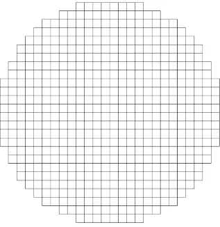
particles are defined by an explicit stair-step grid (material grid hereafter) which freely moves on the background Eulerian grid where the solution is sought. Figure 1 shows the material grid points used to define the particle. Using this explicit grid, particle volume fractions on the background Eulerian grid can efficiently be calculated by using the discrete delta functions [15]:

Θp(x) = Nm X

m=1

δh

x−Xm

h

υm ∀x∈gh. (7)

whereNm, υm andgh are the number of material control volumes, volume of

the m-th material CV and the support of the discrete delta function respec-tively. Also note that Xm refers to the position of the m-th material grid

point. The discrete delta function, δh, is defined by

δh(r) =

1 hd

d

Y

i=1

φ(ri), (8)

where d is the dimensionality of the Eulerian grid, h is the Eulerian grid spacing andri = (xi−Xm,i)/h. There are several choices for the functionφ(r)

in Eq. (8), one such function with reasonable smoothing and computational efficiency [13] is the following function first suggested by Roma et al. [23]:

φ(r) =              1 3 1 +

√

1−3r2

, |r| ≤0.5

1 6

5−3|r| −p1−3(1− |r|)2_{, 0.5<|r| ≤1.5}

0, |r|>1.5.

(9)

The buoyancy forcefB,i in Eq.(3) can be written by [15]:

where subscript T is used to refer to the current temperature. Using a Boussinesq approximation, Eq.(10) can be rearranged to get the following equation for the total body force

fB,i =−(ΘpβpρpT + (1−Θp)βfρfT)(T −Tref)gi+ (ρ−ρf)gi. (11)

In Eq.(11), β is the coefficient of volumetric expansion which is a constant for each phase.

2.1.1. Source correction

The SIMPLE [5, 26] algorithm on collocated grid is used for the pressure velocity coupling which is an iterative process. A second order backward difference in conjunction to the implicit Euler method are used for the time integration of the temporal and spacial terms respectively [15]. Denoting the predicted value of the body force at the current iteration by f_{F D,i}∗ a correction force f_{F D,i}0 can be defined such that f_{F D,i}∗ +f_{F D,i}0 is the required force to impose the rigidity constraint in the particle domain at the current time step. This correction force can be written by [15]:

f_{F D,i}0 (x) =

Nm X

m=1

F_iF D(Xm)δh

x−Xm

h

υm ∀x∈gh. (12)

The required body force on the material grid points FF D

m,i ≡ FiF D(Xm), can

be calculated by

F_m,iF D =ρp

UR m,i−U

∗ m,i

∆t , 1≤m≤Nm, (13)

where

U_m,i∗ = X x∈gh

u∗_i(x)δh

x−Xm

h

and u∗_i are the fluid velocities at the current iteration. The rigid velocity of the individual material points U_m,iR is given by [15]:

U_m,iR =Up,i+ijkωp,j(Xm,k−Xp,k), 1≤m ≤Nm, (15)

where linear (Up,i) and angular (ωp,i) velocities of the particle are calculated

from U_m,i∗ using the principles of conservation of angular and linear momen-tum, see [15] for details. Also note that the a subscript ‘p’ (1 ≤ p ≤ Np)

refers to the particle centres whereas a subscript ‘m’ (1 ≤ m ≤ Nm) refers

to the material points forming that particle. In Eq.(15), ijk is the usual

permutation symbol which is equal to 1 for even permutations of ijk,−1 for odd permutations and 0 otherwise. The freely varying particle temperature is obtained directly from the solution of Eq.(4) and no further treatment is required.

2.2. Collision strategy

When considering more than one particle or when a particle comes too close to a wall, a forcing term should be implemented to prevent particles from overlapping other particle domains or penetrating the domain walls. Simulating the particle collision in fully-resolved methods is the subject of significant research. A widely used method to consider particle-particle col-lision or particle-wall colcol-lision is to calculate the distance between each pair of particles after the particle positions are updated. Then a type of short range repulsive force is calculated for the pth particle by

F_p,iC =

Np X

q=1

q6=p

Fqp,i+ Nw X

w=1

where Nw is the number of domain walls and Np is the number of particles

in the domain. Superscript C is used to indicate the sum of all collision forces on particle pand subscript `p, iis used to indicated the collision force in direction i exerted by object ` on particle p. Object ` can be another particle or a wall which are indicated by q and w respectively. The collision forces F`p,i on p-th particle can be modelled using a short range repulsive

force which following Glowinski et al. [6, 7, 8] can be defined by:

Fqp,i =ξqp(Xq,i−Xp,i)

max

0,Dq+Dp

2 + ∆−dqp

2

, (17)

where dqp is the distance between particle pair (q, p) and ∆ is the range of

activation of the force. Particle-wall collisions are determined by creating a mirror imagep0of the particlepon the other side of the wall, i.eFwp,i =Fp0_p,i. Note that the adjustable parameter xipq is dimensional and has a dimension

of force per unit volume. In this study identical values are used for the dimensional adjustable parameters ξqp for all the particle pairs. Despite the

easy implementation of Eq.(17), there are generally a few issues associated with it. First issue is that the adjustable parameter is problem dependent and is not known a priori. However, a series of numerical experiments which will be detailed in Section 3.1, show that a value of ξqp = 2×106 can be

used for the simulations in this paper for a particle density of ρp = 1.1 and

collision Stokes numbers of St ≥ 10, where no rebound occurs and all the particle kinetic energy dissipates in fluid [2, 10]. The collision Stokes number St is defined by [10]

with Re=ρf|Up −Uf|Dp/µf. This value is in the range of values [105,107]

used in other immersed boundary (IB) [25] and FD simulations [7, 8]. It is worth mentioning again that the value of ξpq is problem dependant and is

adjusted for the current simulations. However, if for a particular problem one sets the value of adjustable parameter such that for St≈10 no rebound occurs then that can be regarded as the correct physics of the problem. In addition, if collision is of the main concern then more accurate (and more expensive) models such as those suggested in [16] should be adopted.

Second issue is that the range of activation of the repulsive forces should be chosen carefully in the current FD method. The choice of ∆ is restricted by the support of the delta function used in this study. In the current method both the rigidity constraint and the divergence free criteria are corrected and therefore both criteria are fulfilled to the required precision. Therefore a slight overlap of the domains is equivalent to requiring the fulfilment of two different constraints at the same grid point which causes the failure of the iterative process. Therefore a value of ∆ = 3h is used in this study. Finally, this repulsive forcing function is continuous and its value grows as d decreases, where d is the separation distance defined in Eq.(17). There-fore using this equation, requires very small time steps such that the force increases continuously in a few steps. Required step sizes, are prohibitively small due to the iterative nature of the current implementation. Therefore the following integration technique is adopted for the current method.

In this approach first the time step is divided into a number of smaller sub-steps using ∆tk = ∆t/Nk where Nk is the number of sub-steps. The

particle using

X_p,ik =X_p,ik−1+U_p,ik ∆tk, (19)

where the superscript k = 1 corresponds to the values at the previous time step (n−1) and k = Nk corresponds to the updated values at the current

time step (n). Also note that Xp,i refers to the centre of the individual

particles which is different fromXm,i used to define the centre of the material

grid points that constitute each particle. In addition in this study we only consider circular particles and hence, only the particle centres are considered to identify the colliding pairs. Total collision force for each particle is then calculated using Eq.(16) and Eq.(17). The position of the particle is corrected using the calculated force by

X_p,ik =X_p,ik−1 + 1 4Mp

F_p,iC,k +F_p,iC,k−1∆t2_k, (20)

and the velocities by

U_p,ik =U_p,ik−1+ 1 2Mp

F_p,iC,k+F_p,iC,k−1∆tk, (21)

where Mp is the total particle mass. At the end of this time integration,

total movement of the particle is calculated by ∆Xp,i =Xp,iNk−X n−1

p,i and the

particle velocities are updated by

U_p,in = ∆Xp,i

∆t . (22)

These velocities are then used to calculate U_m,iR as explained in Section 2.1.1. The rigid velocitiesUR

m,i, are then used to provide the initial estimates for the

also that Un

p,i is calculated only once at the beginning of each time step

using this procedure, however, during the iterative procedure it is calculated using the conservation of linear momentum as explained in Section 2.1.1. In addition the current collision model only exerts normal forces in the direction of the line connecting the centres of particles, therefore it does not directly influence the angular velocity of the particles ωp,i. In addition, the position

of the material grid points Xm are updated using the particle centre position

and the rotation tensor [9] which are updated after each time step [15]. The collision strategy is activated during the particle position update of the FD algorithm [15] and can be summarized as follows:

• For each particle ‘p’ identify the colliding pairs (i.e. the set of particles ‘q’ for which (Dq+Dp)/2 + ∆−dq,p >0).

• Update the positions for sub time step ∆tk using Eq. (19).

• Calculate the collision force between the colliding pair ‘qp’ using Eq. (16).

• Using the calculated collision force recalculate the centre position using Eq. (20) and velocities by Eq. (21).

• For the numerical consistency at the end of the final sub time step re-estimate the particle velocities using Eq. (22).

3. Results and discussions

GPGPU acceleration is considered for the parallelization of the code and the results are presented in Appendix A. Also note that, a CGS system of units is assumed in this paper except otherwise stated. In this section first the collision strategy explained in Section 2.2 is validated using the problem of two settling particles. The benchmark is also extended to consider the case where natural convection takes place from the leading particle. Then the motion of particles in a cavity is considered where critical Grashof numbers are identified and the effects of particle motion on the wall heat transfer properties are discussed.

3.1. Particle-particle collision

In this section sedimentation of two particles at a low Stokes number in a 2D channel filled with a Newtonian fluid is studied to validate the current particle collision strategy. A cavity with height 6 and width 2 is considered and the particle diameters are set to D = 0.2 which are released at y= 0.5 and y= 5.3. Fluid density, density ratio, gravitational acceleration and fluid viscosity are set toρf = 1,ρp/ρf = 1.1,g =−981 andµf = 0.08 respectively.

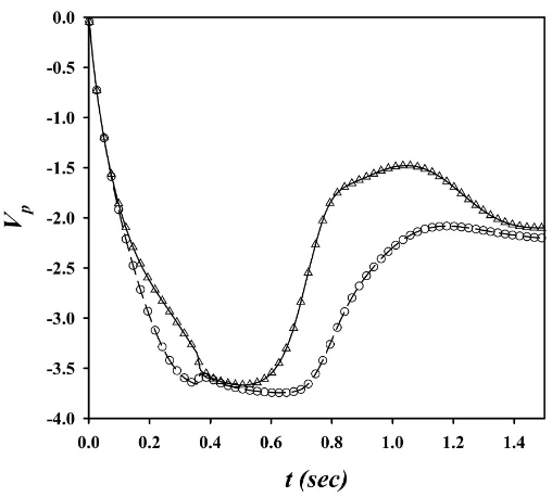
These properties are commonly used for this problem and are adopted here merely to compare the results to other benchmark solutions [2, 25]. The Reynolds number based on the fluid properties and maximum velocity of the trailing particle is 9.68 and the corresponding Stokes number is St = 1.18. Particles are initially displaced by 0.004D as suggested in [2, 25] to let the instabilities to grow during the short collision time. Figure 3 summarizes the motion of the two particles during the course of collision. Results of the Up and Vp are compared to the previous study [2] and very good agreement

only be compare qualitatively. It is discussed in [25] that the motion of the particle after the collision is a manifestation of the strong instabilities in the motion of particles and hence given different collision strategies and different numerical methods significant differences in the particle motion after the collision are expected, which is also reported in [2]. However, given that a different collision strategy is used in this study, the general behaviour of the curves after the collision are similar to those reported in [2] with only a time lag of about 4.91τp whereτp =ρpD2/(18µf).

Overtaking the trailing particle happens att = 0.81 and can be identified from the intersection of the two graphs in Figure 3(d). The base simulation is performed on a grid with uniform spacing, h = 1/256, and a time step size of ∆t = 0.002. To examine the time and grid independence of the collision strategy two other grid resolutions with h = 1/192 and h = 1/320 and one smaller time step of 0.001 are used. In Figure 3 results of all these simulations are also presented. This shows that particle motion even after the collision is indeed, time and grid independent and only depends on the order of the accuracy of the method used. The number of sub time steps is set to Nk= 5 in this study and the independence of the results from this choice

is demonstrated by solving the same problem for the finest grid (h= 1/320) and Nk = 10 and the results of this test are presented in Figure 4.

Similar problem is further considered by initializing the bottom particle to a hotter temperature, TH, and allowing for natural convection from the

particles. A Grashof number based on the particle diameter is defined by

GrD =

ρ2_(T

H −T∞)gβfD3

µ2 . (23)

different Grashof numbers GrD ∈ {100,500,1000,2000} are considered by

changing the βf and no thermal expansion is considered in the particle

do-main, i.e. βp = 0. Particles are initially displaced similar to the case of pure

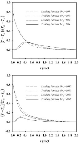
sedimentation discussed earlier in this section. All the other parameters re-main the same and particle temperature varies freely in time. Figure 5 shows the variation of the mean temperature ¯T defined by

¯ T =

Nm X

m=1

Tmυm/ Nm X

m=1

υm, (24)

for the leading and trailing particles in time. At lower Grashof numbers the trailing particle follows the leading particle for a longer time and hence the the temperature of the trailing particle exceeds that of the leading particle at t = 0.45 for GrD = 100 and t = 0.53 for GrD = 500. However for the

larger Grashof numbersGrD = 1000 and GrD = 2000 the mean temperature

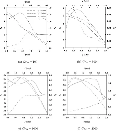
of the trailing particle never exceeds that of the leading particle due to a fast upward motion induced by the natural convection from the bottom particle. Figure 6 shows the time history of the position of the particles at the four different Grashof numbers. At the lowest Grashof number GrD = 100,

the time history of the position of the particle does not significantly differ from the pure settling case presented in Figure 3. However at GrD = 500 no

tumbling is observed. Figure 7 shows the z-vorticity contours superimposed on the temperature contours for the four different cases just before the first collision. At GrD = 100 only a single dominant vortex is observed which is

Figure 6(b) shows the time history of the particle positions at GrD = 500

where no tumbling is observed. This seems to be due to the formation of a pair of counter rotating vortices around the particles, see Figure 7(b), which are not strong enough to lift the leading particle and only have a stabilizing effect on the motion of the trailing particle. Therefore although collisions happen during the course of motion, these secondary vortices prevent the instabilities to grow. AtGrD = 1000 andGrD = 2000, the secondary vortices

are strong enough to lift the leading particle. Contrary to the case ofGrD =

500 where both particles were actually settling in this case the leading particle is moving upward and is pushing the trailing particle up which is by nature unstable, see Figures 7(c) and 7(d). Therefore instabilities do grow in these two cases which results in tumbling of the particles and eventually the two particles separate, see Figures 6(c) and 6(d).

3.2. Motion of particles in a cavity

In this section, particle motion in a 2D DHC is studied in detail. A cavity with sidesL= 1 is considered and is discretized withN = 1000 nodes in each coordinate directions. For the first test case three rows of identical particles are uniformly laid on the bottom wall giving a total of N = 129 particles. Following physical properties (CGS system) are used for the test cases

• µf = 0.01, ρf = 1, ρp

ρf = 1.1, • κf

κp =

1

5, cpf = 10,

cpf

cpp = 5, • Dp = 0.02, g =−981.

A Grashof numberGrL, based on the cavity side lengthLis defined similar to

flow induced by the natural convection. Also note thatTH is the temperature

of the hot wall in this case. The range of Grashof numbers considered here is comparable to the values used in [1] and [22] with air as the operating fluid. In addition, the gravitational effects are determined by the Archimedes number Ar =gD3_ρ

f(ρp −ρf)/µ2, which specifies the fluidization and sedimentation

behaviour of the particles, that are the main concerns of this paper. The Archimedes number for the current system isAr = 7.85 which is comparable toAr= 3.27 for 36µmspherical particles used in [22]. It should, however, be noted that a full examination of all these parameters is outside the scope of the current paper and only the effects of the Grashof number is considered. The Prandtl number based on fluid properties P r = cpfµf/κf, is set to

P r = 0.7 in this study and is kept constant for all simulations. Rayleigh numberRaL=P r·GrLcan be used to summarize all the variable that affect

the large scale motions, however since P r is a constant in this study all the results are reported based on the GrL.

We first investigate the motion of the particles at differentGrL numbers.

By performing several numerical experiments we have identified critical GrL

numbers that significantly effect the patterns of particle motion. Figure 8(a) shows the bed of particles at the bottom of the cavity att= 5 after the start of the calculation with GrL = 5×105. At this Grashof number the strength

This figure clearly shows that at the bottom, due to the larger conductivity, κp, of the particles and smaller specific heatcpp, a significant amount of heat

diffuses into the bed via the near wall particles which significantly changes the local heat transfer behaviour. The particle effects on the heat transfer properties are further discussed in Section 3.3. Figure 8(b) shows the escape mechanism of the particles. It seems that one of the escape mechanisms is due to the net effects of two flow generated torques acting on the particle, one generated from the large scale eddies and one from the upward flow generated due to natural convection from the lower layers of hot particles. These two forces generate a rotation with an off-centre axis of rotation which can roll the particles up its neighbours.

The behaviour of the system remains the same up toGrL = 106 where lift

forces induced by the large scale motions can lift the particles near the hot wall. To better present the behaviour of the system, the following averaging is performed on the position of the particles. The domain is divided into equal number of bins in x- and y-directions and the number of particles in each bin is calculated at each time step. Then the number of particles in each bin is averaged during the sampling period (ts−t0) to yield an average

particle per cell defined by

Nbin=

Pts

t=t0Nbin∆t

ts−t0

, (25)

where t0, ∆t and Nbin are the time at the start of the sampling, time step

Figures 9(a) and 9(b) show the particle position and z-vorticity contours for GrL = 106 and GrL = 2×106 at t = 20 respectively. The first critical

Grashof number is at GrL = 106 where a few particles escape the bed and

move up the hot wall. However the large scale eddies are still not strong enough to sustain the particles in suspension and the particle start to fall on average at a distance of Lf ≈ 16Dp, see also Figure 9(c). In addition, note

that the particles almost exactly follow the path of the leading particles due to a mechanism explained in Section 3.1. However examination of the local vorticity contours shows that no significant flow forms near the particles due to the natural convection. Figure 10 shows the temperature contours in a box specified in Figure 9(b). Particle specific heat is smaller than the fluid’s in this study with a larger thermal conductivity (κp/κf = 5) which means that

the particle quickly attains thermal equilibrium with the surrounding fluid and effectively push the temperature contours away from each other. Due to this local thermal equilibrium with the surrounding fluid, no significant local convection is observed. Although thermal properties of the particles may affect this behaviour no parametric study is performed in this paper. At largerGrL= 2×106 similar behaviour is observed except that the falling

distance of the particle can be as large as Lf ≈25Dp, see Figure 9(d).

Streamlines in Figures 9(a) and 9(b) show that a local eddy can form due to the upward motion of the particles near the hot wall and the free fall of particles at the falling distance Lf. This local eddy gets stronger

at GrL = 2×106 and traps some of the particles. Therefore the expected

Note that in this case, Nbin, is calculated on 21 initially allocated bins from

y = 0.18 in the y-direction, which is the height of the settled particles. In addition, Nbin is further interpolated on a 4 times finer grid which is merely

done for a better presentation.

Figure 11 shows four different stages of particle-particle collision forGrL=

2×106. Particles colliding on top of a row of particles (Particle labelled B

in Figure 11) exerts a normal force with no tendency to rotate particle C. However these settling particle have significant linear momentum which is transferred to the colliding particle (particle C) through a thin layer of fluid between the two particles which exerts a torque on particle C and rotates this particle. It should be noted that only a normal force is modelled in this study and tangential forces are neglected. Therefore, in real physical system friction between neighbouring particles in the row, may quickly deteriorate or even prevent the rotation of particle C. In any case this type of collision does not seem to excite the particle to escape from the bed. However the particle settling at a lower layers (particleA) slide on these layers and collide with the row of particles just in front of them. This collision transfers linear momentum to the row which can excite new particle to escape the bed by generating an upward flow between the particle gaps. Note that the settling particles have both angular and linear momentums (both roll and slide), whereas the particles already on a row, mainly gain angular momentum due to the flow induced torques (only roll), see Figure 8(b).

The Grashof number is further increased to GrL = 5×106 which is the

GrL = 107. Note that in this figure the whole domain is represented since

all particles are fluidized because of the strong large scale eddies. At GrL=

5×106 _{two distinct regions start to develop. A circulation region near the}

hot wall forms similar to the mechanism described for the lower Grashof number cases. Additionally a high concentration region is formed at the top left of the circulation region where some particles get trapped between a large negative vortex and the wall, See Figures 12(a) and 12(b). In addition, increasing the Grashof number seems to push the particles more toward the hot wall and more effectively circulates the particle specially on top left corner where particle motion becomes sluggish. This clustering of particles is significantly different from the results presented in earlier studies [1] where one-way coupled tracer particles are used. In the limiting case of tracer particle, they sample a larger segment of the cavity comparable to the size of the large scale eddies whereas here, particles accumulate near the hot wall due to the particle falling and drafting effects which can produce strong local eddies.

To further test if this clustering behaviour depends on the initial config-uration of the bed we perform another test at GrL= 5×105 with an initial

population of randomly distributed particles (both in x- and y-directions) in the domain. Figure 13 shows the particle distribution at three different times for this case. Evidently the initial configuration of the particles has no effect on the clustering behaviour and they still tend to cluster near the hot wall.

3.3. Particle effects on the wall heat transfer properties

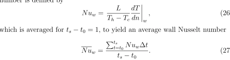
number is defined by

N uw =

L Th−Tc

dT dn w , (26)

which is averaged for ts−t0 = 1, to yield an average wall Nusselt number

N uw =

Pts

t=t0N uw∆t

ts−t0

. (27)

Note that in Eq.(26),n is the wall normal direction and the averaging time is chosen such that the particle circulate once around the local eddy. Figure 14 shows the local value of the Nusselt numberN uw, along the vertical hot wall

of the cavity. AtGrL = 5×105 a significant increase in the value of the local

Nusselt number is observed where the particles reside. This is due to the fact that the local isotherms are pushed toward the hot wall which causes a large local temperature gradient, see Figure 8(d). However in the gaps between the particles the value of the local Nusselt number is significantly reduced to values even below that of an empty cavity. This phenomena is more pronounced in Figure 14(b) where a significant reduction in the heat transfer performance aty <0.2 is obvious. This due to the fact that the heat transfer mechanism is solely conduction dominated in this region whereas large scale eddies could remove a significant amount of heat from the wall if a heap of particles had not been accumulated on the bottom left corner. The local Nusselt number is further averaged along the hot wall to yield

N uw =

PL

y=0N uw∆y

L . (28)

Figure 15 shows the average Nusselt number defined by Eq.(28) for four different Grashof numbers. At GrL = 5×105 although the heat transfer in

more significant than the reduction in convective heat transfer. Additionally particles act as additional sources and the net effect is an increase in the total wall Nusselt number, see Figure 15. At GrL = 2×106 this reduction in

strong convective heat transfer is more important and hence the overall heat transfer rate is significantly reduced.

At two higher Grashof numbers this heap effects are limited to y < 0.05 and hence do not seem to significantly affect the total Nusselt number. How-ever as discussed in the previous section a high particle concentration region is formed on the top left corner of the cavity where particle become slug-gish and similar to the heap effects reduce the eddy strength on that region. This adversely affects the Nusselt number in this region which can be seen in Figures 14(c) and 14(d) at around y = 0.58 and 0.64 respectively. Obvi-ously this region is smaller and particle buoyancy effects are less significant for GrL = 107 and hence the total Nusselt number eventually increases, see

Figure 15.

4. Concluding remarks

In this paper a novel fictitious domain method is used to study the fun-damental mechanisms of the particle motion in a differentially heated cavity. A collision strategy is implemented and tested by considering the settling of two particles in a quiescent flow. This benchmark problem is extended by considering the natural convection from the hot leading particle and criti-cal Grashof number, based on the particle diameter, are identified for this motion.

Motion of the particles in a cavity is then studied by considering three rows of particle initially laying on the bottom of the cavity. Three different flow regimes are identified depending on the Grashof number which is defined based on the domain length scale. Particle fluidization mechanism is studied and the roll of particle collision in exciting new particles to scape the bed is discussed in detail by considering different types of particle-particle collisions. Additionally it is found that the body forces induced by particles settling in large scale eddies can generate smaller local eddies which in turn cause the particles to accumulate near the hot wall and almost certainly will always remain in one half of the cavity. Finally the augmentation mechanism is explained in detail and it is shown that for large particles adding particle may adversely affect the heat transfer properties of the wall.

methods can be used for laboratory scale simulation if combined with con-ventional domain decomposition techniques. These techniques combined by a hierarchical modelling strategy seems to be the best approach for large scale simulations in the foreseeable future, c.f. Haeri and Shrimpton [11] for a suggestion on such hierarchies.

Acknowledgement

The authors acknowledge the use of the IRIDIS-3 High Performance Computing Facility, and associated support services at the University of Southampton, in the completion of this work.

References

[1] Akbar, M.K., Rahman, M., Ghiaasiaan, S.M., 2009. Particle transport in a small square enclosure in laminar natural convection. Aerosol Science 40, 747–61.

[2] Ardekani, A.M., Dabiri, S., Rangel, R.H., 2008. Collision of multi-particle and general shape objects in a viscous fluid. Journal of Com-putational Physics 227, 10094–107.

[3] Buchberg, H., Catton, I., Edwards, D., 1976. Natural convection in en-closed spaces - a review of application to solar energy collection. ASME Journal of Heat Transfer 98, 182–8.

[5] Ferziger, J.H., Peric, M., 2002. Computational Methods for Fluid Dy-namics. Springer.

[6] Glowinski, R., Pan, T., Hesla, T., Joseph, D., Priaux, J., 2001. A ficti-tious domain approach to the direct numerical simulation of incompress-ible viscous flow past moving rigid bodies: Application to particulate flow. Journal of Computational Physics 169, 363–426.

[7] Glowinski, R., Pan, T.W., Hesla, T., Joseph, D., Periaux, J., 2000. A distributed lagrange multiplier fictitious domain method for the simula-tion of flow around moving rigid bodies: applicasimula-tion to particulate flow. Comput. Methods Appl. Mech. Engrg 184, 241–67.

[8] Glowinski, R., Pana, T.W., Hesla, T., Joseph, D., 1999. A distributed lagrange multiplier/fictitious domain method for particulate flows. In-ternational Journal of Multiphase Flow 25, 755–94.

[9] Goldstein, H., Poole, C., Safko, J., 2000. Classical Mechanics. Addison Wesley.

[10] Gondret, P., Lance, M., Petit, L., 2002. Bouncing motion of spherical particles in fluids. Physics of fluids 14, 643–52.

[11] Haeri, S., Shrimpton, J., 2011. A mesoscopic description of polydis-persed particle laden turbulent flows. Progress in Energy and Combus-tion Science 37, 716–40.

[13] Haeri, S., Shrimpton, J., 2012b. On the application of immersed bound-ary, fictitious domain and body-conformal mesh methods to many par-ticle multiphase flows. International Journal of Multiphase Flow 40, 38–55.

[14] Haeri, S., Shrimpton, J.S., 2013a. A correlation for the calculation of the local nusselt number around circular cylinders in the range 10 ≤

Re ≤250 and 0.1≤ P r ≤40. International Journal of Heat and Mass Transfer 59, 219–29.

[15] Haeri, S., Shrimpton, J.S., 2013b. A new implicit fictitious domain method for the simulation of flow in complex geometries with heat trans-fer. Journal of Computational Physics 237, 21–45.

[16] Kempe, T., Frohlich, J., 2012. Collision modelling for the interface-resolved simulation of spherical particles in viscous fluids. J. Fluid Mech , 445–89.

[17] Kissane, M.P., 2008. On the nature of aerosols produced during a severe accident of a water-cooled nuclear reactor. Nucl Eng Des 238, 2792–800.

[18] Korpela, S.A., Lee, Y., Drummond, J.E., 1982. Heat transfer through a double pane window. Journal of Heat Transfer 104, 539–44.

[19] Kuerten, J.G.M., van der Geld, C.W.M., Geurts, B.J., 2011. Turbu-lence modification and heat transfer enhancement by inertial particles in turbulent channel flow. Phys. Fluids 23, 123301–8.

[21] Patankar, N., Singh, P., Joseph, D., Glowinski, R., Pan, T.W., 2000. A new formulation of the distributed lagrange multiplier/ fictitious domain method for particulate flows. International Journal of Multiphase Flow 26, 1509–24.

[22] Puragliesi, R., Dehbi, A., Leriche, E., Soldati, A., Deville, M., 2011. Dns of buoyancy-driven flows and lagrangian particle tracking in a square cavity at high rayleigh numbers. International Journal of Heat and Fluid Flow 32, 915–31.

[23] Roma, A., Peskin, C., Berger, M., 1999. An adaptive version of the immersed boundary method. J. Comput. Phys 153, 509–34.

[24] Tiwari, R.J., Das, M.K., 2007. Heat transfer augmentation in a two-sided lid-driven differentially heated square cavity utilizing nanofluids. International Journal of Heat and Mass Transfer 50, 2002–18.

[25] Uhlmann, M., 2005. An immersed boundary method with direct forcing for the simulation of particulate flows. Journal of Computational Physics 209, 448–76.

[26] Versteeg, H., Malalasekra, W., 2007. An Introduction to Computational Fluid Dynamics: The Finite Volume Method. Prentice Hall.

Appendix A. Code acceleration on GPU

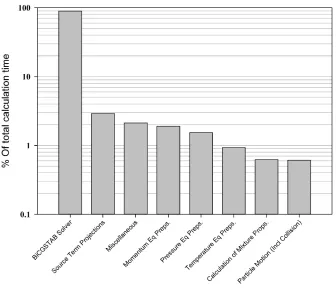
The first step in a GPGPU parallelization strategy is to time the code and identify the possible candidates for the GPU acceleration. Timing is per-formed using the code profiling tools provided by the Intel Parallel Studio and the DHC problem, which is discussed in detail in Section 3.2. Figure A.1 shows the results of the code timing. Clearly the single function that can benefit the most from the GPU acceleration is the linear solver which ap-proximately consumes 90% of the total CPU time.

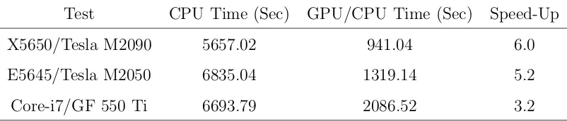
In this study a Krylov sub-space type iterative solver namely BiCGSTAB [27], is used to solve the linear equations resulting from the discretization of the momentum, pressure and temperature equations. The main algorithm is im-plemented using the C language and the cuSPARSE and cuBLAS libraries. Fortran 2003iso c bindingfeature is used to interface the C function and to call the solver from the main Fortran code. The first test is performed on the Iridis-31 compute nodes which are equipped with 2.4GHz Intel Xeon E5645 processors and NVIDIA Tesla 20-series, M2050, GPGPU co-processors and approximately 22GB memory. The second test is performed on the Emerald GPU cluster2_{. The Emerald comprises 60 HP SL390 compute nodes with two}

6-core X5650 Intel Xeons, three 512-core M2090 NVIDIA GPUs and 48GB of memory, in addition 24 high memory nodes with 96GB memory and eight M2090 NVIDIA GPUs are available. The last test is performed on an Intel

1_{University of Southampton supercomputer facility ranked 331 on Top500 list on}

November 2012.

2_{Emerald is a large HP GPU system utilising 372 NVIDIA Tesla processors hosted at}

Core i7-2600 workstation with a midrange GeForce GTX 550 Ti and 16Gb of memory. The Cuda SDK 4.2.9 and the Intel Fortran Compiler are used for compiling and linking the code on both systems. All the test on each system are performed with exactly the same set of compiler options, namely

Test CPU Time (Sec) GPU/CPU Time (Sec) Speed-Up

X5650/Tesla M2090 5657.02 941.04 6.0

E5645/Tesla M2050 6835.04 1319.14 5.2

Core-i7/GF 550 Ti 6693.79 2086.52 3.2

Fig. A.1: Time spent in different functions during the course of a sample run. 90% of the

calculation time is spent in the iterative solution of the linear system using the BiCGSTAB

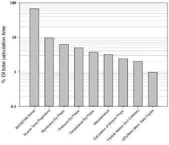
Fig. A.2: Time spent in different functions during the course of a sample run after GPU

Fig. 1: Stair-step grid used for the discretisation of the particle. The depicted grid is much

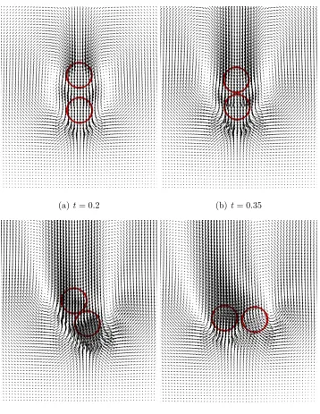
(a) t= 0.2 (b)t= 0.35

(c) t= 0.65 (d) t= 0.8

Fig. 2: Vector plots of two colliding particles for Stp = 1.18 - Three different stages of

(a) Vertical velocity (b) Lateral velocity

(c) Angular velocity (d) Vertical position

Fig. 3: Linear and angular velocity and vertical position of the two particles atStp= 1.18

- Time and grid independence of the collision strategy is tested. — Leading particle

(∆t = 0.002, h = 1/256), — — Trailing particle (∆t = 0.002, h = 1/256), --- Leading

particle (∆t = 0.002, h = 1/320), — - Trailing particle (∆t = 0.002, h = 1/320), -·-·

-Leading particle (∆t= 0.002,h= 1/192), -··-··- Trailing particle (∆t= 0.002,h= 1/192),

4 Leading particle (∆t= 0.001,h= 1/256),◦ Trailing particle (∆t= 0.001,h= 1/256),

Fig. 4: Independence of the results (h= 1/320) from the number of sub-steps. — leading

particle Nk = 5, — — trailing particleNk = 5, 4 Leading particle Nk = 10, ◦ Trailing

(a) GrD= 100 (b)GrD= 500

(c) GrD= 1000 (d) GrD= 2000

Fig. 6: Time history of the particle positions for four considered Grashof GrD numbers.

No tumbling is observed for Gr = 500 and upward collision is observed for Gr = 1000

and Gr = 2000. Horizontal positionsxp should be read from the right and top axis and

(a) GrD= 100, t= 0.45 (b) GrD= 500, t= 0.25

(c) GrD= 1000, t= 0.2 (d) GrD= 2000, t= 0.2

Fig. 7: 26 levels ofωzare superimposed on 40 levels of temperature contours. Temperature

contours are presented for 0<( ¯T−T∞)/(TH−T∞)<0.4 for all the cases and dashed lines

(a) Stream Lines (b) Vector plot

(c) Temperature Contours (d) Temperature Contours

Fig. 8: Particle behaviour in the DHC at GrL = 5×105 at t = 5. Magnified vector

and contour plots show the particle in a region specified by a box in the corresponding

(a) GrL = 106 (b) GrL= 2×106

(c) Nbinat GrL= 106 (d) Nbin atGrL= 2×106

Fig. 9: Particle behaviour in the DHC above the critical Grashof number GrL = 106.

Vorticity contours and stream lines are plotted atts= 20 and the positions are averaged

betweent0= 8 andts= 20. Position averaging starts at the heigh of the settled particles

y = 0.18 for a better presentation. Vorticity contours are presented betweenωz =−190

Fig. 10: Temperature contours near particles in the region specified in Figure 9(b) by a

Fig. 11: Escape of a new particle from the bed due to the collision and momentum transfer

along the raw of the particles. Frames are labelled 1· · ·4 and ∆t between the frames is

(a) GrL= 5×106 (b) GrL= 107

(c) GrL= 5×106,Nbin (d) GrL= 107,Nbin

Fig. 12: Particle behaviour in the DHC above the critical Grashof numberGrL= 5×106.

The positions are averaged between t0 = 8 and ts = 20 for GrL = 5×106 and between

t0 = 6 and ts = 18 for GrL = 107 and vorticity contours are presented at ts. Vorticity

Fig. 13: Instantaneous Nbin, for randomly distributed particles in the cavity at GrL =

(a) GrL= 5×105 (b) GrL= 2×106

(c) GrL= 5×106 (d) GrL= 107

Fig. 14: Variation of the local wall Nusselt number along the hot wall at four different