City, University of London Institutional Repository
Citation
:
Gashi, I., Popov, P. T. and Stankovic, V. (2009). Uncertainty explicit assessment
of off-the-shelf software: A Bayesian approach. Information and Software Technology, 51(2),
pp. 497-511. doi: 10.1016/j.infsof.2008.06.003
This is the unspecified version of the paper.
This version of the publication may differ from the final published
version.
Permanent repository link:
http://openaccess.city.ac.uk/514/
Link to published version
:
http://dx.doi.org/10.1016/j.infsof.2008.06.003
Copyright and reuse:
City Research Online aims to make research
outputs of City, University of London available to a wider audience.
Copyright and Moral Rights remain with the author(s) and/or copyright
holders. URLs from City Research Online may be freely distributed and
linked to.
City Research Online:
http://openaccess.city.ac.uk/
[email protected]
Bayesian Approach
Ilir Gashi, Peter Popov, Vladimir Stankovic
Centre for Software Reliability,
City University,
Northampton Square
London EC1V 0HB
United Kingdom
Tel: 020 7040 0273, 020 7040 8963, 020 7040 0273,
Fax: 020 7040 8585
http://www.csr.city.ac.uk
{I.Gashi, V.Stankovic}@city.ac.uk,
{ptp}@csr.city.ac.uk
Abstract. Assessment of software COTS components is an essential part of component-based software
development. Poorly chosen components may lead to solutions of low quality and that are difficult to
maintain. The assessment may be based on incomplete knowledge about the COTS component itself and other
aspects (e.g. vendor’s credentials, etc), which may affect the decision of selecting COTS component(s). We
argue in favor of assessment methods in which uncertainty is explicitly represented (‘uncertainty explicit’
methods) using probability distributions. We provide details of a Bayesian model, which can be used to
capture the uncertainties in the simultaneous assessment of two attributes, thus, also capturing the
dependencies that might exist between them. We also provide empirical data from the use of this method for
the assessment of off-the-shelf database servers which illustrate the advantages of ‘uncertainty explicit’
methods over conventional methods of COTS component assessment which assume that at the end of the
assessment the values of the attributes become known with certainty.
Keywords: COTS component assessment, reliability and performance assessment, Bayesian inference
1. Introduction
The use of commercial-off-the-shelf (COTS) components in software development is ubiquitous. There are
many benefits to using COTS components stemming from the incentive to cut down on cost and development
time and to improve quality by using tried and tested components. An essential part of component-based
software development is the assessment of available COTS components. Various assessment methods have been
proposed [1], [2], [3], [4], [5], [6], [7], [8], [9], [10], [11], [12], [13], [14]. The results of these assessment
techniques crucially depend on assuming that the values of the assessed attributes will be known with certainty
at the end of the assessment. However, since the assessment is carried out with limited resources of time and
We propose an assessment method, in which the assessment results are subject to explicitly stated uncertainty
and discuss how this may impact the selection of COTS software. The method also enables representing the
dependencies that exist between the uncertainties associated with the values of the COTS component attributes,
which affect the decision about which of the available COTS components to choose. It also encourages assessing
the dependent attributes simultaneously, thus identifying the dependencies that may exist between the values of
the attributes which may affect the choice of component(s). We provide empirical results from a study with
off-the-shelf database servers, which demonstrate how the assessment method can be used in practice.
The paper is structured as follows: section 2 contains a brief review of related work on COTS component
assessment and attribute definitions; section 3 contains an overview of the problems that need to be addressed
during COTS component assessment; in section 4 we describe models of assessment, in which model parameters
(values of the attributes to be assessed) are not known with certainty and argue in favor of using probability
distributions as an adequate mechanism to capture this uncertainty; in section 5 we give details of an empirical
study with off-the-shelf database servers and also some contrived numerical examples, which illustrate the
advantages of handling uncertainty and dependence between the values of the attributes; section 6 contains a
discussion of the scalability and applicability of the method proposed; and finally in section 7 we present
conclusions and possible further work.
2. Related Work
2.1 COTS Assessment Methods
There is a wide variety of COTS component assessment approaches available. All of them start with an initial
statement of requirements, which defines what is being sought. It has been proposed that the requirements
initially should not be too stringent, since this would discard potentially appropriate COTS component
candidates at a very early stage [9], [15]. It has even been suggested [15] that if the requirements are not flexible
then the COTS-based development may not be appropriate and bespoke development could be more
cost-effective. So initially [15] suggests distinguishing between essential requirements and those that are negotiable.
The selection criteria are then based on the essential requirements.
Off-the-shelf-option (OTSO) [2] is a multi-phase approach to COTS component selection. The phases are: the
search phase, the screening and evaluation phase and the analysis phase. In the first phase COTS components are
identified. In the screening and evaluation phase the components are further filtered using a set of evaluation
criteria (established from a number of sources, including the requirements specification, the high level design
specification etc.). In the analysis phase results of the evaluation are analyzed, which lead to the final selection of
COTS components for inclusion in the system. Other similar multiphase process approaches for COTS
component evaluation that have been proposed include CEP (Comparative Evaluation Process Activities) [7],
CBA Process Decision Framework [8] which in addition to defining a process for COTS component assessment
also defines two other processes: COTS integration (“gluing”) and COTS configuration (“tailoring”);
CAP-COTS Acquisition Process method [5] and PECA Process [13].
Procurement-oriented requirements engineering (PORE) [1] is a process in which requirements are defined in
concerning COTS components and their use within the wider system. Other methods that are centred on the
requirements to assist with the COTS component selection process are CRE-COTS-Based Requirements
Engineering Method [6], Storyboard Process [11], Combined Selection of COTS Components [12] and
COTS-DSS [14].
CISD (COTS-based Integrated System Development) [4] and CDSEM (Checklist Driven Software Evaluation
Methodology) [3] are both checklist-based evaluation methodologies. STACE (Socio Technical Approach to
COTS Evaluation) [10] is a socio-technical approach to evaluation which builds on work of [1] and [2] and
emphasizes the organizational issues related to COTS selection.
2.2 Attribute Definition Methods
Extensive work has been also reported on definition of COTS component assessment attributes. A
comprehensive list is given in [16]. They group the attributes in two categories depending on how they can be
measured: Attributes Measurable at Runtime (which contain Accuracy, Security, Recoverability, Time Behavior
and Resource Behavior) and Attributes Measurable during Component Life-Cycle (Suitability, Interoperability,
Maturity, Learnability, Understandability, Operability, Changeability, Testability and Replaceability). These
attributes are further divided into more fine-grained attributes, which are measurable using their proposed
metrics of: presence, time, level and ratio. This work [16] follows the spirit of the guidelines for attribute
definitions outlined by the international standardizing organizations ISO [17], and IEEE/ANSI [18] in a broader
context, not specific to COTS component attributes. COCOTS framework by Abts et al. [19], and Torchiano and
Jaccheri [20] also provides COTS attribute definitions.
3. Problems with COTS Component Assessment
3.1 Motivation
Any assessment is conducted with limited resources and under various assumptions, which may not hold true in
real operation. As a result the outcome of the assessment is subject to uncertainty – the assessor may never be
100% sure that what they concluded during the assessment (both about the values of the attributes as well as the
choice of a COTS component) will be confirmed when the COTS component is used in operation. This is clearly
true for some parameters, which can be estimated objectively, e.g. failure rate, performance, etc. For failure rate,
for instance, even after a very thorough testing one can only identify a range of rates which are more likely than
others. For instance, Littlewood and Wright have shown [21] that starting with indifference between the values
of the failure rate (i.e. uniform distribution of the failure rate in the range [0, 1]) and seeing a protection system
process correctly 4603 demands translates into 99% confidence that this system’s probability of failure on
demand (pfd) is no worse than 10-3. The same equally applies to attributes assessed subjectively, e.g. using the
Likert scale [22], widely used in the COTS component assessment. It may be difficult for an assessor to justify
that a COTS component must be ranked at exactly, say 7 out of 10, according to a chosen scale but he/she may
The value of expressing the assessment results in the form (value, confidence) has been recognized in some other
technical areas which dealt with assessment. The best performing software reliability-growth models (RGM)
which predict the failure rate from the observed failures in the past, for instance, are those in which the model
parameters are treated as random variables [23]. In these models the ‘true’ values of the attributes being assessed
are never assumed known with certainty. Instead the attribute is characterized by a probability distribution, from
which the true value of the attributes will come (i.e. are seen as drawn at random). For each reliability target,
then, the assessor can tell the probability that the true reliability is lower than the target. Such models
systematically outperformed the alternative simplistic methods in which the parameters were assumed to be
known with certainty [24]. If the ‘uncertainty explicit’ models have been best with one specific method of
assessment – software reliability – it seems natural to try similar ‘uncertainty explicit’ methods for other
assessments, e.g. evaluation of COTS software and selecting the best out of a set of comparable alternatives.
This is the focus of this paper.
There are various methods for representing uncertainty [25]. Bayesian approach to probabilistic modelling is one
of the best-known ones and used with some success in reliability assessment [24], [21]. It allows one to combine,
in a mathematically sound way, the prior belief (which may be ‘subjective’) about the values of a parameter or a
set of parameters to be assessed with the (‘objective’) evidence from seeing the modelled artefact in operation.
Combining the prior belief and the evidence from the observations in a mathematically correct way leads to a
posterior belief about the values of the assessed attribute(s).
How does ‘uncertainty explicit’ assessment differ from the conventional deterministic assessment? With
deterministic assessment point estimates of the attributes are used. A common approach of comparing the
alternatives is then to use a weighted sum of the estimates for each of the alternatives. When uncertainty is
accounted for, this approach is still possible – we can use various characteristics of the posterior distributions
(mean, median, etc.) of the attributes as estimates and then calculate the weighted sum for each of the COTS
components included in the assessment before deciding which is the best one. When uncertainty is explicitly
used in the assessment, however, more refined ways of comparison are possible: from the posterior one can
express the uncertainty in the value of the comparison criterion, e.g. the weighted sum of the attributes. Since
the value of the weighted sum is now uncertain we have a range of options. We may give preference to the
COTS component for which the mean (median) value of the weighted sum is the best (as we would have done
with point estimates of the attributes). With uncertainty stated explicitly a range of new options exists, which is
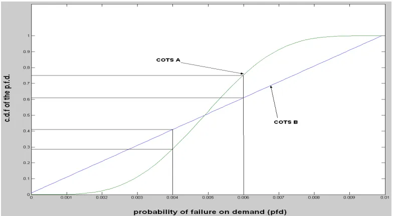
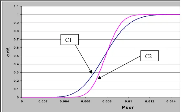
Fig. 1 - The pfd for two different COTS components
In this figure we illustrate the value of handling uncertainty explicitly even when dealing with a single
assessment attribute, COTS component reliability. Let us assume that Fig. 1 illustrates the cumulative
distribution function (c.d.f.) graph for two COTS components with the same average pfd. If we wanted to
choose the COTS component that has the highest probability of having a pfd of no worse than 6*10-3 (i.e. the
value of the x-axis of 0.006) then we would choose COTS component A, whereas the COTS component with the
highest probability of having a pfd of no worse than 4.10-3 is COTS component B. We can also see clearly that
the distribution of the pfd of COTS component B is much more spread than that of COTS component A (in fact
the distribution of COTS component B is uniformly spread across all the values from 0 to 10-2). Therefore there
is a much higher uncertainty associated with the values of COTS component B than that of COTS component A.
Stating uncertainty explicitly offers the assessor a wider range of options in selecting the most appropriate COTS
component.
3.2 Dependence among Attributes
COTS component assessment requires dealing with multiple attributes of the COTS components being
compared. The selection of a particular COTS component, thus, is a multi-criteria decision which taken under
uncertain values of the attributes naturally leads to the question about the dependence between the uncertainties
associated with the individual attributes. Ignoring the possible dependence between the uncertainties in
attributes’ values represents a particular form of belief: that assessing attribute X one can learn nothing about
another attribute, Y. For example, performance of a COTS component will hardly tell anything about the quality
of its documentation and vice versa. It is quite obvious, however, that not all COTS component attributes are like
that. In many cases while assessing an attribute X the assessor may infer something about the values of another
set of attributes. For instance, if we devise a prototype in order to assess the functionality of a COTS component
we will also learn something about the performance (how quickly this COTS component responds to requests)
and how reliable the COTS component is. A more subtle, but very useful concept, as we will see later, is that the
assess the reliability and performance of a COTS component. We may assume that the uncertainties associated
with these two attributes are independent, in the statistical sense. Under this assumption learning something
about reliability will tell us nothing about performance and vice versa. Now suppose that we have run a very
long testing campaign and have repeatedly observed that whenever the response was late it was also incorrect
and no other incorrect response has been observed. With such evidence of a strong positive correlation between
the failures (incorrect responses) and the responses being late, we may accept that any change of our belief about
the rate of failure should also be translated into a change in our belief about the rate of late responses. The
assessment models surveyed invariably assume that the values of the attributes are independent and do not allow
for dependencies between their uncertain values to be captured adequately.
In summary, with the assessment method that we propose in this paper we aim to handle both the uncertainties
in the values of the attributes and the dependence that exists between the values of the different attributes. The
existing assessment methods we surveyed do not deal explicitly with either of these two uncertainties.
4. Assessment of COTS Components: a Bayesian Approach
In this section we briefly summarize how the Bayesian approach to assessment is normally applied to assessment
of a single attribute. Assume that the attribute of interest is the component’s probability of failure on demand
(pfd). If the system is treated as a black box, i.e. we can only distinguish between COTS component’s failures or
successes, the Bayesian assessment proceeds as follows. Let us denote the system pfd as p, with prior
distribution (probability density function, pdf)
f
p(
•
)
, which characterises the assessor’s knowledge about theCOTS component pfd prior to observing the COTS component in operation. Assume further that the COTS
component is subjected to n demands, independently drawn from a ‘realistic’ operational environment (profile)1,
and r failures are observed. The posterior distribution,
f
p(
x
|
r
,
n
)
, of p after the observations will be:)
(
)
|
,
(
)
,
|
(
x
r
n
L
n
r
x
f
x
f
p∝
p , (1)where
L
(
n
,
r
|
x
)
is the likelihood of observing r failures in n demands if the pfd were exactly x, which in thiscase of independent demands is given by the binomial distribution,
x
rx
n rr
n
x
r
n
L
−
−
=
(
1
)
)
|
,
(
. For anyprior and any observation (r, n) the posterior can be calculated2 for all the COTS components included in the
assessment. Even if no failure is observed (i.e. r = 0), the posterior can be calculated. Other measures of interest
can also be derived from this posterior, e.g. the probability that the COTS component will survive the next 5000
1 An operational profile [26] can be defined as a statistically accurate characterization of how the component will be used in
its ‘true’ environment.
2 The posterior can be calculated either by using a conjugate prior distribution [27], in which case the posterior distribution is
guaranteed to be in the same family as that of the prior for a given likelihood function (e.g. Beta distribution prior, with
Binomial Likelihood function, gives us a Beta distributed posterior) or it can be calculated through numerical methods and
approximations. In our case, since the conjugate family has limitations [28] we have used numerical methods to calculate
randomly chosen demands. This probability can be calculated for each of the COTS components included in the
assessment as follows:
(
)
(
)
∫
∞−
05000
,
|
1
p
f
pp
r
n
dp
.Then the best COTS component will be the one, for which the integral above gets a maximum value.
4.1. A Model for Assessment of 2 Non-Independent Attributes
Typically, COTS component assessment is a multi-criteria decision with dozens of attributes usually assessed
and taken into account (as detailed in [2], [1], [5], [8]). The Bayesian assessment can be applied to multiple
attributes, too. For simplicity we first demonstrate the approach with two attributes and then discuss (in section
5) the implications of scaling it up to many attributes. A similar model to the one we describe here has been used
in the past in assessing reliability of various systems built with components [28], [29].
Let us assume that two non-functional attributes must be assessed, such as the COTS component’s pfd and
performance, the latter assessed in the form of whether the response is received on time or not, i.e. the
probability of a late response on demand, pld. Using a binary score – on time vs. late – is an adequate approach
when the COTS component is planned for integration in a larger system. In these circumstances using an
absolute scale, e.g. how long it takes a COTS component to respond to a demand, may be unnecessary: it will be
sufficient to know whether the response is received with an acceptable delay as dictated by the wider system. In
terms of comparison of several COTS components using the binary scale (on time/late) seems also adequate.
Any COTS component, which responds with an acceptable delay, is sufficiently good from the point of view of
the system’s integrator.
Here we define a model to help with the comparison of COTS components assessed by subjecting them to a
series of independently selected demands. Both, the COTS component’s pfd and pld, are used in the comparison
and different comparison criteria are discussed.
On each demand the response received from the COTS components is evaluated from two different viewpoints:
correct/incorrect and on time/late. Clearly 4 combinations exist, which can be observed on a randomly chosen
demand, as shown in Table 1.
Table 1 – The outcomes, their frequencies and probabilities for a random demand.
Event Correct Response (Reliability)
Response On-Time (Performance)
Number of observations in
n demands Probability
α No Yes r1 p10
β Yes No r 2 p01
χ No No r 3 p11
δ Yes Yes r 4 p00
The four probabilities given in the last column sum to 1. So if the first three probabilities are 0.2, 0.4 and 0.3,
respectively, then the last one
p
00 = 1 - (0.2 + 0.4 + 0.3) = 0.1. This constraint remains even if we treat theof these parameters, e.g.
(
,
,
)
11 10
01,p ,p
•
•
•
pf
, gives an exhaustive description of the COTS component’sbehaviour. In statistical terms, the model of the COTS component with two binary attributes has three degrees of
freedom.
The marginal probabilities of getting an incorrect response on a random demand, let’s denote it pI, and of getting
the response late, pL, respectively, can be expressed as:
11 10
p
p
p
I=
+
andp
L=
p
01+
p
11.p11 represents the probability of receiving late an incorrect response. Hence, the notation pIL ≡ p11,
11 10
p
p
p
I=
+
andp
L=
p
01+
p
11will capture better the intuitive meaning of the event it is assigned to.Instead of using
(
,
,
)
11 01
10,p ,p
•
•
•
pf
another distribution, which can be derived from it through a change ofvariables [30], can be used. In this section we use , ,
(
•
,
•
,
•
)
IL L
I p p
p
f
which can be factorised as:)
,
|
(
)
,
(
)
,
,
(
, ,,p p p p p I L
p
f
f
p
p
f
IL L I IL LI
•
•
•
=
•
•
•
(2)For the prior joint distribution ,
(
•
,
•
)
L I p p
f
above, we assume throughout this paper that the pI and pL areindependently distributed3. We capture the possible dependencies between the two failures processes
(characterized by pI and pL, respectively) by | ,
(
•
)
L IIL p p
p
f
. Hence the full joint prior distribution is given by:)
,
|
(
)
(
)
(
)
,
,
(
,,p p p p p I L
p
f
f
f
p
p
f
IL L I IL LI
•
•
•
=
•
•
•
(3)For a given observation (r1, r2, and r3 in N demands) the posterior joint distribution can be calculated as:
∫∫∫
=
IL L I IL L I IL L I IL L I p p p IL L I p p p IL L I p p p p p pdxdydz
p
p
p
r
r
r
N
L
z
y
x
f
p
p
p
r
r
r
N
L
z
y
x
f
r
r
r
N
z
y
x
f
, , 3 2 1 , , 3 2 1 , , 3 2 1 , ,)
,
,
|
,
,
,
(
)
,
,
(
)
,
,
|
,
,
,
(
)
,
,
(
)
,
,
,
|
,
,
(
(4) where 3 2 1 3 21
(
)
(
1
)
)
(
)!
(
!
!
!
!
)
,
,
|
,
,
,
(
3 2 1 3 2 1 3 2 1 r r r N L I IL r IL r IL L r IL I IL L Ip
p
p
p
p
p
p
p
r
r
r
N
r
r
r
N
p
p
p
r
r
r
N
L
− − −−
−
+
−
−
−
−
−
=
(5)is the multinomial likelihood of the observation (r1, r2, r3 , N).
4.2. Combination of Uncertainties in the Values of Attributes
For comparison of the COTS components we will define the following criterion:
Probability of an inadequate response, PSer, by the COTS component: of getting either an incorrect or late
response. Clearly, PSer= PI + PL – PIL. Its posterior distribution,
f
(
|
N
,
r
1,
r
2,
r
3)
Serp
•
, can be derived from
the joint posterior,
f
, ,(
,
,
|
N
,
r
1,
r
2,
r
3)
IL L
I p p
p
•
•
•
, by first transforming it, to for example)
,
,
,
|
,
,
(
1 2 3,
,
N
r
r
r
f
Ser L
I p p
p
•
•
•
, and then integrating out the nuisance parameters PI and PL.An often used selection method [31] in the literature is the weighted sum of the values of the attributes. The
weighted sum of the two attributes in our study can be calculated as follows: PS= kPI + (1-k)PL, in which the
constant k is defined by the assessor in the range 0-1. High values of k correspond to cases when incorrect results
are highly undesirable while late results may be tolerable. On the other hand, low values of k correspond to cases
when incorrect results may be tolerated by the system while late responses may have serious consequences. In
order to derive the marginal distribution of PS first the joint distribution
f
, ,(
,
,
|
N
,
r
1,
r
2,
r
3)
ILL
I p p
p
•
•
•
istransformed to
f
, ,(
,
,
|
N
,
r
1,
r
2,
r
3)
S L
I p p
p
•
•
•
and then the nuisance parameters PI and PL are integrated out,as above for PSer. However we will not be using this method of selection since the new variable PS does not have
an obvious intuitive meaning. The difficulty is compounded in our case since the uncertainty is stated explicitly.
It is impossible to say what a confidence of say 99% associated with a particular value of PS tells us about the
COTS component being assessed.
4.3. Partitioning the Demand Space
In some areas of software engineering, especially in testing, the usefulness of partitioning the demand space has
been recognised [32], [33], [26]. The demand space partitions typically represent different types of demands,
which may have different likelihoods of occurring in a realistic environment. Realistic testing, thus, would
require generating mixes of demands, which take into account the likelihood of the types of demands.
In our context, operating in a partitioned demand space may imply that the uncertainty associated with the
attributes of interest may differ among the partitions, e.g. as a result of different number of observations being
made for the different partitions.
If the demand space is partitioned into M partitions {S1, S2, … SM}, with a probabilistic measure { P(S1),…,
P(SM)} 4, then for each of these the assessment will be performed as described above, e.g. with two attributes the
description provided in section 4.1 will apply. As a result M conditional distributions will be associated with
each COTS component, e.g. using reliability and performance these can be denoted as
f
p ,p ,p(
,
,
|
S
i)
IL L
I
•
•
•
,from which the conditional distribution fp ( |Si)
Ser • will be expressed. This distribution characterises the
probability of failure (incorrect or late response),
P
Ser|
S
i, of the particular COTS component in the specific partition. Finally, in order to compare the competing COTS components the unconditional distribution)
(
•
Ser p
f
should be derived for the particular profile defined over the set of partitions, which represents thetargeted operational environment.
4 The meaning of these random variables is that a demand chosen at random with probability P(S
Let us assume the profile of the targeted environment is known with certainty5. The marginal probability of
failure of a COTS component, according to the formula of full probability is:
( )
∑
=×
=
Mi
i i Ser
Ser
P
S
P
S
P
1
|
(6)The distribution of this random variable,
P
Ser, depends on the joint distribution,(
•
,...,
•
)
) | ( ),..., |
(PSer S1 PSer SM
f
, i.e. of the conditional probabilities of failure in sub-domains. In some setups itmay be plausible to assume that the conditional probabilities of failure (in the partitions that is) are independently
distributed, i.e.:
(
)
∏
( )
( )
=
•
•
=
•
•
Mi
S P S
P S
P S
PSer Ser M
f
Serf
Ser Mf
1
| |
) | ( ),..., |
( 1
,...,
1...
. (7)Such an assumption represents the assessor’s belief that learning something about the probability of failure,
i Ser
S
P
|
, of a particular COTS component in partition i will not change their belief about the probability of failure,P
Ser|
S
j, of the same COTS component in another partition. The assumption is consistent withapplying inferences to the individual partitions, i.e. conditional on the demands coming from a particular
partition.
Under (7) the unconditional probability of COTS component failure (6) can be expressed as a convolution of the
distributions of the random variables
P
w( )
i
=
P
Ser|
S
i×
P
( )
S
i , i.e.:( )
i
P
P
Serw=
⊗
w (8)The selection of the best COTS component, out of the available alternatives, will then be based on the marginal
distributions, w
(
•
)
Ser pf
, associated with the available COTS components.5. Numerical Examples: a Study with Off-The-Shelf Database Servers
We have reported recently results of studies on dependability and performance of database servers [34], [35],
[36], [37]. The focus of these earlier studies was in measuring the amount of “diversity”, in both correctness and
response time, which exists between different servers, i.e. certain servers might give an incorrect and/or late
response in one input but the others might not. The motivation behind this work was to get preliminary
measurements on the improvements in reliability and performance that can be had from using more than one
component in parallel in a multi-channel diverse configuration.
In this paper we will use the data collected in those studies to demonstrate our approach to COTS component
selection. SQL servers are a very complex category of off-the-shelf components, with many reported faults in
5 This assumption is needed for the comparison only. We do not require here that we know the ‘real’ operational
environment, in which the system together with the chosen COTS component will be deployed. Taking into account the
uncertainty about the profile is possible at the expense of making the calculations more complicated, which is beyond the
each release. In total six off-the shelf SQL servers from four different vendors were used. Four of the servers are
open-source, namely PostgreSQL 7.0, PostgreSQL 7.2, Interbase 6.0 and Firebird 1.06. The other two servers are
commercial closed development servers, anonymised here due to the restrictive ‘End User License Agreements’.
We will refer to these components as CS1 (Commercial Server 1) and CS2 as they are from different vendors.
An ideal selection of an SQL server based on the results of statistical testing of the COTS components may be
problematic in practice. We will highlight two circumstances in which these difficulties can occur:
-Assume that we are interested in choosing between several SQL servers, based on their reliability and
performance. The ideal situation for choosing the most appropriate SQL server based on measurements after
deploying the COTS components is clearly unrealistic since we would like to select the best server before the
application is developed.
-Assume that the system integrator (e.g. a software house) would like to make a strategic choice of a SQL
server for use in the foreseeable future. In this scenario the application(s), which may be developed in the
future may be even unknown at the time of making the selection.
Given these difficulties we can use alternative options:
- Use well-known benchmark applications. In the context of SQL servers this might be the TPC-C benchmark
for on-line transaction processing [38]. In this case, the performance of the components can be measured
directly on the target platform, but there might be problems observing failures. This is because it would be
reasonable to expect that an SQL server would correctly process the statements defined in the TPC-C
benchmark application. Thus, in this case the selection of the SQL server would be significantly influenced
by the performance attribute. Even if failures are observed, such a measurement of the reliability of the
COTS components may be very expensive; the likely candidates to choose from will be reliable components.
Thus the amount of testing to observe a few failures may be prohibitively high [39]. We illustrate the
assessment method with data collected from experiments with an implementation of the TPC-C client
benchmark. For the TPC-C experiments we used all six aforementioned SQL servers.
- Use stressful environments (in terms of the reliability attribute) for comparing the components, i.e.
environments which increase the likelihood of failures occurring, even if we do not know how likely these
are to occur in operation. The set of bugs of a particular COTS component (in our case SQL server) defines
one such stressful environment for a server. The union of the bugs reported for all the compared COTS
components will form a demand space, in which there will be a partition stressing each of the components.
We have collected known bug reports for four of the SQL servers in our studies, namely PostgreSQL 7.0,
Interbase 6.0, CS1 and CS2 and used them as a sample from a ‘stressful’ environment, in which to compare
the COTS components.
Detailed results for each of these studies are given in the next two sub-sections. We did not use partitioning of
the demand space approach in the study with the TPC-C benchmark application (even though the TPC-C
transactions types could form basis for such partitioning). This is because we did not have any reason to expect
that the servers will perform differently (in terms of timeliness and correctness) for each transaction type. We
however did use partitioning of the demand space in the study with the bug reports of the servers, since we had
compelling reasons to expect that the servers will perform differently (this will be explained in section 5.2).
6 Firebird is the open-source descendant of Interbase. The later releases of Interbase are issued as closed-development by
5.1 Study with TPC-C Benchmark Application
We first describe the results obtained using the TPC-C benchmark application as a basis of selecting the best
SQL server. In the empirical study we used our own implementation of TPC-C. The benchmark defines five
transaction types (New-Order, Payment, Order-Status, Delivery and Stock-Level) and sets the probability of
execution for each, i.e. the particular transaction mix (profile) is defined. The specified performance measure is
the number of New-Order transactions completed per minute. However, our measurements were more detailed -
we recorded the transaction response times instead. The benchmark specifies an upper bound on the 90th
percentile values for each transaction type. It requires that the average response time of each transaction type is
less than or equal to the respective 90th percentile value. The values are as follows:
-New-Order - 5 seconds
-Payment - 5 seconds
-Delivery – 80 seconds
-Order-Status – 5 seconds
-Stock-Level – 20 seconds
The test harness consisted of two machines:
-A server machine, on which one of the six database servers was run.
-A client machine, which executed a JAVA implementation of the TPC-C standard.
Each experiment comprised the same sequence of 1000 transactions. We ran two types of experiments:
-single client - a TPC-C compliant client modifies the database by executing the specified transaction mix.
-multiple clients - a TPC-C compliant client modifies the database and additional 10 clients concurrently
execute the read-only transactions (Order-Status and Stock-Level).
Multiple clients experiment enabled us to increase the load on the servers and measure the effect of the increased
load on their performance.
A timeout value, specific to each transaction type, was used to distinguish between late and timely responses.
We defined two sets of timeouts7:
-The 90th percentile values specified by TPC-C (TPC-C timeout),
-One fifth of the 90th percentile values (shorttimeout).
We defined four scenarios, varying the number of clients and timeout values respectively:
-Scenario 1 - single client / TPC-C timeouts
-Scenario 2 - single client / short timeouts
-Scenario 3 - multiple clients / TPC-C timeouts
-Scenario 4 - multiple clients / short timeouts
The SQL servers were compared for each of the scenarios.
7 The choice of these was made after a personal communication of one of the authors with a TPC-C affiliate and auditor who
5.1.1 Prior Distributions
The prior, , ,
(
•
,
•
,
•
)
IL L
I p p
p
f
, was constructed under the assumption that PI and PL are independentlydistributed random variables, i.e. ,
(
•
,
•
)
=
(
•
)
(
•
)
L I L
I p p p
p
f
f
f
. We made this assumption since we did nothave any objective evidence to believe otherwise. In case there are reasons (objective or subjective) then the
assumption of independence may be dropped. In this case the particular form of ,
(
•
,
•
)
L I p p
f
should be definedexplicitly. Additionally the conditional distributions
f
p |P,P(
|
P
I,
P
L)
L I
IL
•
were defined for every pair ofvalues of PI and PL, in the range [0, min(PI, PL)] since the probability of incorrect and late responses cannot be
greater than the probability of either of the two individually. In passing we note that the choice of the prior is not
critical with the benchmark application since an arbitrarily large number of demands can be generated, i.e. ‘the
data will speak for itself’.
We anticipated observing mainly late responses while the incorrect result failures were expected to be very rare.
We have assumed ‘ignorance prior’ (Uniform distribution) for performance in the range
P
L∈
[
0
,
1
]
. For incorrect result failures we have also assumed ignorance but using an upper bound of 10-2, likely to be veryconservative in the context of TPC-C, i.e. we used the range
P
I∈
[
0
,
10
2]
. We assumed ignorance priors for both PI and PL since we did not have any preference regarding their values. In this study we used the samedistribution for all the servers since for the scenarios tested we did not have any reason to prefer one server over
the others. There might, however, be cases – some discussed later in section 6.4 - whereby the assessor may have
different prior beliefs about the competing COTS components.
[image:14.612.115.491.428.517.2]A summary of the distributions used and the range in which they are defined is given in Table 2.
Table 2 - The Prior distributions (identical for all six servers and all four scenarios).
Prior Distribution Range Distribution Type
Reliability (•)
I p
f 0 – 0.01 Uniform
Performance (•)
L p
f 0 – 1 Uniform
Conditional distribution: fpIL|pI,pL(•|PI,PL) 0 – min(PI,PL) Uniform
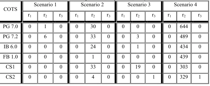
5.1.2 Observations
The observations from the TPC-C experiments are given in Table 3. The number of demands for all servers is
1000. Five out of six servers exhibit late result failures only. Incorrect result failures are observed only for CS2.
In addition, whenever a result was incorrect on CS2 it was late, too. The incorrect results observed were due to
the specific concurrency control mechanism used by CS2 [34]. The locks on resources, e.g. database rows, were
not released properly when the lock holding transactions were completed. To resolve the problem we had to
install timeout watchdogs and abort transactions when the timeout expired. Each aborted transaction was
repeated as many times as necessary to eventually commit successfully. We decided to use transaction repetition
count as the criterion of an incorrect response on CS2. In particular, we defined a threshold of 5 as the value,
beyond which the transaction would be considered to have failed.
We used transaction timeout values and transaction repetition count to classify each demand on each server in
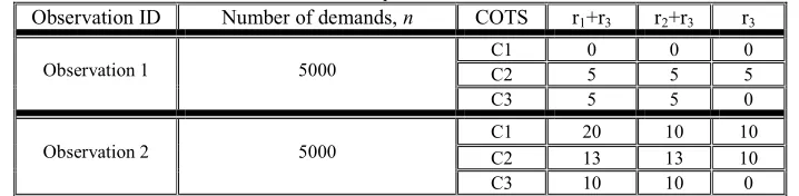
Table 3 - The observations of the six database servers for the four scenarios. The number of demands (n) is 1000 for each server. We did not observe any incorrect-only failures, i.e. r1=0 for all servers.
Scenario 1 Scenario 2 Scenario 3 Scenario 4
COTS
r1 r2 r3 r1 r2 r3 r1 r2 r3 r1 r2 r3
PG 7.0 0 1 0 0 30 0 0 0 0 0 644 0
PG 7.2 0 6 0 0 33 0 0 3 0 0 489 0
IB 6.0 0 0 0 0 24 0 0 1 0 0 434 0
FB 1.0 0 0 0 0 1 0 0 0 0 0 439 0
CS1 0 0 0 0 33 0 0 19 0 0 303 0
CS2 0 0 0 0 4 0 0 0 1 0 329 1
5.1.3 Posteriors
The percentiles derived from the posterior distribution for the 4 scenarios are given in Table 48. One can see that
the ordering between the servers changes as the number of clients and/or the timeout values vary (to improve the
readability of the table we have explicitly shown the ranking order of the servers in each scenario).
Under Scenario 1 (the least demanding scenario) four servers (IB 6.0, FB 1.0, CS1 and CS2) produce identical
results since they completed without any failure (i.e. on time and correctly) the 1000 transactions. We are
indifferent in the choice among them. The two versions of PostgreSQL exhibit late responses and they are
ranked lowest.
When we decrease the timeout value (Scenario 2) the ranking changes: now there are late responses with all the
servers. The two worst servers are CS1 and again PostgreSQL 7.2. Interestingly, Firebird 1.0, an open-source
server, is ranked the best.
In Scenario 3 the percentile values are close again as in the first scenario, though the earlier version of
PostgreSQL, PG 7.0, is ranked the best, alongside Firebird 1.0 while CS1 is the worst performing server.
Firebird 1.0 is consistently among the best servers in the first 3 scenarios. An interesting observation is the 50th
percentile value of the posteriors CS2 and IB 6.0. Even though the total number of failures for these two servers
were the same (1 each, see Table 3), the nature of the failure was different: the result from CS2 was both
incorrect and late whereas from IB 6.0 it was only late. Exploring this dependence we can still see a difference in
the 50th percentile values of these two servers (even though the difference is marginal and on the chosen
accuracy of expressing the percentile values is not observed in the 99th percentile). We will further scrutinize the
interplay between the failures of the individual components and the correlation between their failures with
contrived examples in section 5.4.
The ranking changes again in the most demanding scenario (Scenario 4). The best server is now CS1.
Table 4 – Percentiles (abbreviated P-tile) for the distribution of the system quality PSer = PI + PL – PIL classified per scenario.
To improve the readability we have also provided the ranking order for each of the servers based on the percentiles values. The prior distribution is the same for all servers across all scenarios.
Scenario 1 Scenario 2 Scenario 3 Scenario 4
P-tile COTS Prior
Posterior Rank Posterior Rank Posterior Rank Posterior Rank
PG 7.0 0.0021 5 0.0310 4 0.0012 1 0.6436 6
PG 7.2 0.0071 6 0.0340 5 0.0041 5 0.4888 5
IB 6.0 0.0012 1 0.0250 3 0.0021 4 0.4340 3
FB 1.0 0.0012 1 0.0021 1 0.0012 1 0.4392 4
CS1 0.0012 1 0.0340 5 0.0200 6 0.3032 1 0.5
CS2
0.502
0.0012 1 0.0051 2 0.0020 3 0.3300 2
PG 7.0 0.0076 5 0.0456 4 0.0060 1 0.6780 6
PG 7.2 0.0152 6 0.0492 5 0.0108 5 0.5256 5
IB 6.0 0.0060 1 0.0384 3 0.0076 3 0.4704 3
FB 1.0 0.0060 1 0.0076 1 0.0060 1 0.4756 4
CS1 0.0060 1 0.0492 5 0.0324 6 0.3376 1 0.99
CS2
0.992
0.0060 1 0.0124 2 0.0076 3 0.3652 2
5.2 Study with the Known Bugs of the Servers
Now we compare the servers using the methodology described in section 4.3. We have collected known bug
reports for four SQL servers. We will use the union of the bugs reported for each of these SQL servers. Each of
these bug reports will constitute a ‘demand’ to the server. These demands form a partition of the demand space
for each server9. In contrast to the TPC-C study where partitioning of the demand space was not used, in the
study with the bug reports we apply inferences to the partitions. The reason for doing so was the very different
prior beliefs about the behaviour of servers in the different partitions as will be discussed in section 5.2.1. The
logs of the known bugs are treated as a sample (without replacement10) from the corresponding partition
(representing the server, for which the bug has been reported). We label the partitions
S
Servername. PartitionX
S is called an ‘own’ partition for server X and a ‘foreign’ partition for any other server Y≠X.
9 We have observed no bug reported for two or more servers, thus the logs of the known bugs indeed formed partitions of the
union of the bugs. Even if we had observed bugs reported from more than one server we could construct a partition of the
intersection of the bugs reported for several servers by putting them in their own partition. Thus, a server may have more
than one own partition in the demand space and the description provided here will apply.
10 Strictly, there might be a difference between sampling with and without replacement. Our model is based on sampling
without replacement while the inference procedure described in section 4.1 implies sampling with replacement. This is a
simplification, which in many cases is acceptable (e.g. sampling from a large population of units, none of which dominates
the sampling process, which seems a plausible assumption in our case of SQL servers being very complex products and
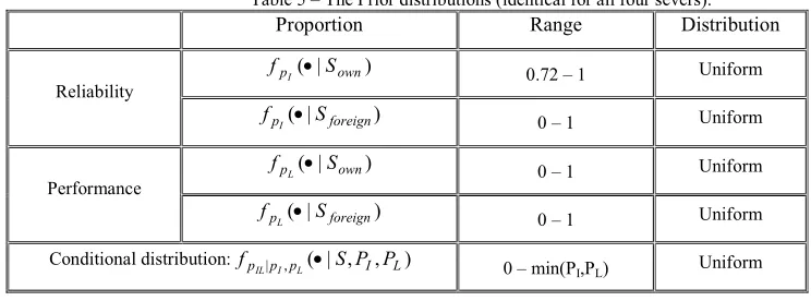
5.2.1 Prior Distributions
The prior distributions fpI,pL,pIL(•,•,•|Si) used in this study are explained next. The prior
distribution, fpI,pL,pIL(•,•,•|Si), was constructed under similar assumptions to those of the TPC-C study: that
PI and PL are independently distributed random variables; in the general case of incorrect and late responses
being non-independent events, the conditional distributions, fpIL|PI,PL(•|Si,PI,PL), are specified for every pair
of values of PI and PL.
The distributions were assumed to be identical for each of the four servers in both their ‘own’ and ‘foreign’
partitions. Again, this assumption was made because we did not have objective evidence to believe otherwise.
We discuss other options in section 6.4. A summary of the distributions used and their respective parameters
including the range of each distribution are given in Table 5, and we will discuss these choices in the rest of this
[image:17.612.119.491.267.405.2]sub-section.
Table 5 – The Prior distributions (identical for all four severs).
Proportion Range Distribution
) | ( own
p S
f
I • 0.72 – 1 Uniform
Reliability
) |
( foreign
p S
f
I • 0 – 1 Uniform
) | ( own
p S
f
L • 0 – 1 Uniform
Performance
) |
( foreign
p S
f
L • 0 – 1 Uniform
Conditional distribution: fpIL|pI,pL(•|S,PI,PL) 0 – min(PI,PL) Uniform
Prior distributions for Incorrect ResultsfpI(•|Si)
For ‘own’ partitions the prior distribution was defined as Uniform in the range [L, 1], where L < 1 accounts for
the chance that some of the reported bugs might be Heisenbugs11, i.e. we expect most of the bugs that have been
reported for a particular server to cause failures when they are run on that server (hence the probability of
observing an incorrect results failure is very close to 1) but, due to Heisenbugs, not always so. As a source for L
we used the study by Chandra and Chen [41]. These authors studied the fault reports for three off-the-shelf
components: MySQL database server, GNOME desktop environment and the Apache web-server and reported
that 5%, 7% and 14%, respectively, of the reported bugs were Heisenbugs. Given the variation between the
components we cautiously interpreted these findings by setting L = 1-(2*0.14), that is twice the highest value of
Heisenbugs reported, thus the prior is expected to be within the range [0.72, 1]. Notice that here the prior
distribution for incorrect results is being defined at a range close to 1 (i.e. high unreliability). This is because of
the unusual profile of the demands: since we are using known bug reports as demands we expect most of the
bugs to cause failures when we run them on the server for which they were reported.
For ‘foreign’ partitions, however, the prior distributions were defined as uniform in the range [0, 1]. This is due
to the absence of any comparative study to guide our expectation about the likely value. In passing we note that
11 Gray defines two types of bugs [40]: “Bohrbugs” for bugs that appear to be deterministic (they manifest themselves each
time the bug script is executed); and “Heisenbugs” for those that are difficult to reproduce as they only cause failures under
theoretical work such as [42], [43] suggest that diverse software versions will tend to fail coincidentally on
‘difficult’ demands. Since all the bugs are ‘difficult’ – they are known to be problematic at least for one of the
servers – we may consider them genuinely difficult, hence assume as plausible that the other servers too, are
likely to fail. On the other hand, empirical studies such as [44], [45], have shown that significant gains can be
had via design diversity – hence low chances that a particular server will fail on bugs reported for other server
are also plausible. In summary, we are indifferent between the values of the probability that a server will fail
from a ‘foreign’ bug.
Prior Distributions for Performance fpL(•|Si)
We have not found a public domain source, which would allow us to define a prior distribution for performance
failures (in the context we have defined). This is also because the number of late results that would be observed
would be conditional on how the timeout threshold is set. The only remaining source is to look at the data (either
our own or of various vendors) from the experiments using the TPC-C [38] benchmark. However it is not clear
how reasonable a prior based on these results would be due to the differences in the profile that will exist
between the TPC-C client application and the bug scripts. Therefore we have decided to define the prior
distribution for all proportions as uniformly distributed in the range 0 to 1, i.e. be ‘indifferent’ between the
possible chances of the servers exceeding the set timeout.
Prior Distributions for Incorrect and Late Results fpIL|PI,PL(•|Si,PI,PL)
All conditional prior distributions of the probability of a result being at the same time incorrect and late were
defined in the range [0, min(PI,PL)] (since the probability of incorrect and late responses cannot be greater than
the probability of either of the two individually). This is again due to the rather unique profile, under which we
apply the inference and the lack of comparable studies that would enable us to define different priors than
assuming ‘indifference’.
Priors for Probabilities of a Bug Being Selected From the Partitions
For the comparison of the servers we use a distribution defined on the set of partitions, which does not favour
any of the servers, i.e. we assumed that probability of each partition is 0.25 in the study with 4 servers12.
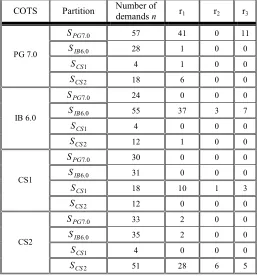
5.2.3 Observations
The observations using the known bugs of four off-the-shelf servers are given in Table 6. We can see that the
number of bugs collected for each server was different, which indicated that the empirical evidence differs
between the partitions. The reasons for this was merely differences in the reporting practices operated by the
vendors of the servers, e.g. unavailability in the public domain of fully reproducible bug scripts for the
commercial servers (especially CS1). Therefore, the sizes of the samples from the partitions on each server are
different. Additionally, these servers are not functionally identical: they offer different degrees of compliance
with the SQL standard(s) and even proprietary extension to SQL. Bugs affecting one of these extensions,
therefore, cannot exist in a server that lacks the extension. In other words, such bug scripts will provide empirical
evidence for the server they were reported for but not for the other servers. We called these “dialect-specific”
12 We could have used the number of known bugs for each of the partition to construct a profile consistent with the
observations. This is not acceptable for two reasons: i) it will favour poor bug reporting practices, and ii) we would have
bugs. Due to this, not all the bugs reported for a server can be run on the other servers. Therefore the number of
‘foreign’ bug reports varies between the servers. The interested reader will find an extensive discussion of the
[image:19.612.177.434.136.413.2]study with the bugs in [37].
Table 6 – The observations for the 4 off-the-shelf servers on the bug reports of the different partitions. In the partition column we have stated for which server these bugs have been reported.
COTS Partition Number of
demands n r1 r2 r3
0 . 7 PG
S 57 41 0 11
0 . 6 IB
S 28 1 0 0
1 CS
S 4 1 0 0
PG 7.0
2 CS
S 18 6 0 0
0 . 7 PG
S 24 0 0 0
0 . 6 IB
S 55 37 3 7
1 CS
S 4 0 0 0
IB 6.0
2 CS
S 12 1 0 0
0 . 7 PG
S 30 0 0 0
0 . 6 IB
S 31 0 0 0
1 CS
S 18 10 1 3
CS1
2 CS
S 12 0 0 0
0 . 7 PG
S 33 2 0 0
0 . 6 IB
S 35 2 0 0
1 CS
S 4 0 0 0
CS2
2 CS
S 51 28 6 5
5.2.4 The Posterior Results
The 50th and 99th percentiles of the marginal distribution, w (•) Ser
p
f 13, associated with each server is shown in
Table 7. Since the prior distributions are identical for each of the components, then the ordering of the
components in the posteriors will be determined by the observations. The best server, across all the percentiles is
CS1. This is not surprising since CS1 did not fail for any of the foreign bugs. The second best server is CS2,
although IB 6.0 is very close, both at the 50% and the 99% level of confidence. This is somewhat surprising at
first given that this server failed more on the foreign bugs than IB6.0. However, the total number of foreign bugs
that could be run on CS2 (72) is much higher than IB6.0 (40). Additionally the number of Heisenbugs for CS2 is
[image:19.612.176.435.138.414.2]also much higher (23.5%) than IB6.0 (14.5%), which leads to the CS2 being better in the posteriors.
Table 7 - The table shows the percentiles of the system quality w (•) Ser
p
f for each server.
Percentiles 0.5 0.99
COTS PG7.0 IB6.0 CS1 CS2 PG7.0 IB6.0 CS1 CS2
Priors 0.77 0.77 0.77 0.77 0.94 0.94 0.94 0.94
Posterior 0.42 0.32 0.24 0.3 0.55 0.45 0.32 0.42
[image:19.612.126.480.591.640.2]
5.3. Discussion of the Results for the Two Setups
We have seen that under the more ‘stressful’ profiles (i.e. Scenario 4 in the TPC-C study and the Bugs study) the
best COTS component is CS1. The fact that we have come to the same conclusion using rather different testing
methods and different profiles would give us an extra assurance that CS1 is indeed the best component for
applications with more stringent reliability and performance requirements which operate at greater transaction
load and level of concurrency. However if the concurrency is low, then even with more rigid performance
requirements (Scenario 2) Firebird 1.0 server, which is open-source and freely available, comes out as the best
server.
The two studies are also in agreement with respect to the worst server – these are the PostgreSQL components.
We could also use the outcome of the studies as a validation of the proposed method. CS1, which came out best,
is widely accepted by the database community to be the best SQL server and has by far the largest share in the
market of SQL servers. This gives some confidence that both the data that we used is sufficiently informative to
allow for meaningful and accurate discrimination between the competing components and the method itself is
trustworthy to provide rigorous ground for accurate COTS component selection.
5.4. Further, Contrived Examples
In the empirical study with the SQL servers we could not fully illustrate the interplay between the dependence
and the uncertainty in the values of the attributes due to the empirical results often being strikingly different for
each server and also because the prior distributions that we started with were the same for each server. In this
section we provide some further numerical examples, which illustrate the usefulness of handling uncertainty and
dependence between the attribute values explicitly. We comment on the cases where the choice of the best
COTS component would differ with conventional assessment methods which rely on point estimates of the
attribute values and make assumptions of independence between the values of the attributes. We also discuss the
effect of the priors on the selection, including different priors for each of the competing components. The choice
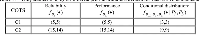
of prior distributions and the observations serve illustrative purposes only. The prior, , ,
(
•
,
•
,
•
)
IL L
I p p
p
f
, wasconstructed under the assumption that PI and PL are both Beta independently distributed random variables,
)
,
,
(
a
b
Beta
•
, defined in the interval [0, 0.01]14, i.e.(
,
)
(
)
(
)
, L
•
•
=
I•
L•
I p p p
p
f
f
f
. The conditionaldistributions,
f
p |p ,p(
|
P
I,
P
L)
L I
IL
•
, for every pair of values of PI and PL are also assumed to be Betadistributions,
Beta
(
•
,
a
,
b
)
. Clearly they are defined in the range [0, min(PI, PL)]. Note that we do not provideany justification for the choice of the prior distributions used here, and neither for the interval on which the
distribution is defined; the particular choice of the type of the prior is dictated by some convenience offered by
Beta distribution in the examples given below. The assessor can choose any prior distribution and interval that
best represents his/her prior beliefs.
14 In all numerical calculations we used the function BETADIST (x, alfa, beta, lowerbound, upperbound) implemented in
many standard libraries, see for instance [46]. The last two parameters, lowerbound, upperbound ∈ [0, 1], define the