Determine Measurement Set for Parameter Estimation in
Biological Systems Modelling
Hong Yue1, Jianfang Jia2
1. Department of Electronic and Electrical Engineering, University of Strathclyde, Glasgow G1 1XW, UK E-mail: [email protected]
2. School of Information and Communication Engineering, North University of China, Taiyuan 030051, P. R. China E-mail: [email protected]
Abstract:Parameter estimation is challenging for biological systems modelling since the model is normally of high dimension, the measurement data are sparse and noisy, and the cost of experiments is high. Accurate recovery of parameters depend on the quantity and quality of measurement data. It is therefore important to know what measurements to be taken, when and how through optimal experimental design (OED). In this paper we present a method to determine the most informative measurement set for parameter estimation of dynamic systems, in particular biochemical reaction systems, such that the unknown parameters can be inferred with the best possible statistical quality using the data collected from the designed experiments. System analysis using matrix theory is introduced to examine the number of necessary measurement variables. The priority of each measure-ment variable is determined by optimal experimeasure-mental design based on Fisher information matrix (FIM). The applicability and advantages of the proposed method are illustrated through an example of a signal pathway model.
Key Words:Measurement Set Selection, Optimal Experimental Design, Parameter Estimation, Biological Systems
1
Introduction
Most mechanistic mathematical models developed for bi-ological and other systems contain adjustable or unknown parameters, the values of which can be estimated from ob-servations. Parameter estimation is challenging for biopro-cesses modelling [1] due to: (1) lack of quantitative mea-surements of dynamic response data and the measurement data is often corrupted with noise; (2) the complex nature of biological systems with high-dimensional, nonlinear and poorly understood dynamics. In general, performing exper-iments to obtain rich data is expensive and time-consuming for such systems. The problem of designing experiments to generate efficient measurement data is thus of particular importance. The term ’optimal experimental design (OED)’ or ’design of experiment’ refers to designing experiments in such a way that the parameters can be estimated from the resulting experimental data with the best possible statistical quality. This is a subject area of growing interests particu-larly in systems biology since huge experimental efforts are required in model development. Various methodologies have been developed and successfully applied to a broad range of systems [2–4]. Interested readers can find comprehensive reviews on experimental design and applications for general systems in [5, 6] and biological and biochemical systems in [7, 8].
The number of unknown parameters is often large for bio-logical system models compared to the limited measurement data, which raises the issue of identifiability. The checking of identifiability is essential in employing parameter estima-tion techniques such as least squares estimaestima-tion, maximum likelihood method and Bayesian estimation, etc [9]. Two types of identifiability are considered: the a priori struc-tural identifiability and theposterioripractical identifiability. Structural (global) identifiability is concerned with the
ques-This work is partly supported by National Natural Science Foundation of China (NSFC) under Grant 61004045, and Research Fund for the Doc-toral Program of Higher Education of China (20091420120007).
tion of the theoretical uniqueness of solutions for a given model and experiment. A nonlinear system is said to be structurally (globally) identifiable if each set of parameter values yields unique output trajectories. This property guar-antees that, under ideal conditions of noise-free observations and error-free model structure, the unknown parameters can be uniquely estimated from the designed input-output ex-periment [10]. The structural identifiability is a theoretical property of the model and a necessary condition for a suc-cessful parameter estimation, however, it is not sufficient to guarantee estimation accuracy in practice [11]. Additional problems commonly encountered in practice are sparse and noisy data, weak effect of unknown parameters on the mea-sured output, etc., which should be addressed in practical identifiability analysis. The identifiability of a parameter estimation problem can be improved through well-designed experiments in general.
In order to produce and collect information-rich data, ex-perimental design can be considered from two aspects. One is the design of input perturbations (type, level and duration of input signals), the other is to determine when and what kind of observations should be taken. Design parameters include level of initial conditions, which input and output variables to be taken, what sampling schedule to follow, etc. In this paper, OED is performed on choosing the most suit-able set of observation varisuit-ables for parameter estimation, also calledmeasurement set selectionin earlier publications [12, 13]. In measurement set selection, we need to consider not only the issue of identifiability in theory, but also the experimental restrictions in biology. For example, in a wet-lab environment, normally only a small number of protein concentrations can be simultaneously measured in a timely fashion. It is therefore important to determine which observ-ables would provide more information for parameter estima-tion. Given a set of unknown parameters to be estimated, we attempt to investigate: (1) the best (minimum) number of measurement variables to be used; and (2) the set of mea-surement variables to be chosen.
The rest of the paper is organized as follows. In Sec-tion 2, the preliminaries on parameter estimaSec-tion and model-based OED is briefly introduced. In Section 3, firstly the general dynamic model is reformulated to improve the com-putational efficiency and facilitate further analysis, then the method to determine the minimum measurement set is dis-cussed using the matrix theory, and the priorities of state variables are calculated by model-based OED. Using a sim-plified IκBα-NF-κB signal pathway model as an example, the applicability of the design method to biological systems modelling is illustrated in Section 4. Finally the conclusions and discussions are given in Section 5.
2
Parameter Estimation and Experimental Design
Preliminaries
Consider a general ordinary differential equation model to describe the dynamics of biological systems
˙
X(t) = f(X(t),p,ω), X(t0) =X0 (1)
Y(t) = h(X(t),p) +ξ(t) (2)
X∈Rnis the state vector with initial conditionX0andnthe number of the state variables. Each component ofXis de-noted asxi, which normally stands for molecule concentra-tions in biochemical system models. p∈Rmis the param-eter vector withmthe number of parameters. The compo-nents ofpmostly refer to kinetic reaction rates.f(·)is a col-umn nonlinear function for states transition, which is often derived from the underlying biochemical mechanisms. The vectorωis introduced to represent the experimental design parameters. Y∈Rris the measurement output vector with
r(r ≤ n)being the number of measurement variables, and
h(·)the measurement function reflecting the choice of ob-servables. The signalξis assumed to be independently and identically distributed, additive, zero-mean Gaussian noise. Parameter estimation for system (1)-(2) can be obtained by the least-square algorithm
ˆ
p = arg min
p∈Θ N
l=1
Y(tl)−Yˆ(ˆp, tl) T
Q−1
Y(tl)−Yˆ(ˆp, tl)
(3)
whereYandYˆ are measurement output and model predic-tion output, respectively.Qis the measurement error covari-ance matrix, the subscriptlindicates sampling time,Nis the total number of sampling points in the dimension of time.
The Fisher information matrix (FIM) quantifies the in-formation content of the measurement data for parame-ter estimation. For a nonlinear dynamic system, the FIM is a nonlinear function of the estimated parameters un-der the assumption that the measurement noise is indepen-dently and identically distributed with a zero-mean Gaus-sian distribution. Denote X = [x1, x2,· · ·, xn]T, p = [p1, p2,· · · , pm]T, the local sensitivity matrix is described as
S=∂X/∂p= (sij), sij =∂xi/∂pj (4) The FIM is represented as a function of local sensitivity ma-trix:
FIM(p,ω) = N
l=1
ST(tl,p,ω)Q−1S(tl,p,ω). (5)
Under the assumption of additive zero-mean Gaussian noise in measurement, an OED problem can be written as a general optimization problem to read
ω∗= arg max
ω∈ΩΦ (FIM(p,ω)). (6) Ωis the design space for the experimental design vectorω, Φ(·)indicates the widely used alphabetical experimental de-sign criteria that are normally scalar functions of FIM, such as A-optimal, maximizing trace(FIM); D-optimal, max-imising det(FIM); E-optimal, minimizingλmax(FIM−1), etc. Here trace(·)anddet(·)are trace and determinant of a matrix,λmax(·)is the maximum eigenvalue of a matrix. These criteria are related to the size and shape of the confi-dence hyper-ellipsoid for estimated parameters, and will give slightly different experimental design results when choosing different criteria. The design using any of the three crite-ria turns out to be a convex optimization problem when the FIM is an appropriate function of the experimental design parameters [14]. Problem (6) is in general an NP-hard prob-lem, and the computational cost of the optimization problem depends on the complexity of the model structure/dynamics.
3
Measurement Set Selection
3.1 Dynamic Model with Unknown Parameters
For a system containing known and unknown parame-ters, the parameter vectorpcan be separated into two sets: η∈Rlfor known parameters, andθ ∈Rqfor unknown pa-rameters withl+q=m. Here it is reasonable to assume that the model is linear in parameters, as widely applied to bio-chemical systems taking kinetic rate coefficients as parame-ters to describe the individual reactions in a model. Consid-ering a simple example of a generic reactionS1+S2−→k P, the reaction rate is given byk[S1]a[S2]b with[·] being the concentration of reaction species, and a, b reaction orders with respect to S1 andS2, respectively. k is the rate con-stant that is a linear term in describing the reaction rate. Un-der this assumption and together with the separation of the known and unknown terms in p, model (1) can be further written as follows (for simplicity,ωis omitted):
˙
X(t) =g(X(t))η+ϕ(X(t))θ (7) whereg(·) ∈ Rn×l andϕ(·) ∈ Rn×q are nonlinear func-tions associated with known and unknown parameters, re-spectively. For a biochemical system, the nonlinear function
g(·)often contains both linear and nonlinear terms with re-spect to species concentrations (state variables). A typical nonlinear form involving two reaction species is a bilinear function. When a system has a large number of reactions, leading to a high dimension in model parameters, the sepa-ration of the linear (states) terms from the nonlinear (states) terms will decompose the model into subgroups with a re-duced size in each group. This will largely improve the efficiency of numerical calculations that often involve inte-gration operation of matrix functions. Following this idea, model (7) is further reformulated to be:
˙
the known parameter vector associated with˜g(·). Note that with this new formulation that isolate the unknown param-eters from the whole parameter set, the termpof the FIM function in (6) should be replaced byθin OED.
3.2 Minimum State Number to be Measured
A general assumption is made thatmeasurement outputY
are linear function of the states. This is how measurement data is processed with most current measurement techniques applied to biological or biochemical systems. The measure-ment output in (2) can then be written as (ignoring the noise term for simplicity)
Y(t) =CX(t) (9) whereC ∈ Rr×n is the measurement matrix. From model (8) and (9), the output reads
Y(t) = CeAtX0+C
t
0
eA(t−τ)˜g(X(τ))dτ
η1
+C
t
0
eA(t−τ)ϕ(X(τ))dτ
θ (10)
Equation (10) shows the linear dependency of measure-ment observables on unknown parametersθ. According to the linear matrix theory, the rank of the linear term multi-plied to θ, i.e. rank
C0teA(t−τ)ϕ(X(τ))dτ should be
maximised in order to realise the minimum number of mea-surement variables for the estimation ofθ. The design prob-lem can then be formulated as an optimisation probprob-lem of choosing a matrixC, consisting of elements 1 or 0, so as to maximise the following objective function:
J(C) = max
C rank
C
t
0 e
A(t−τ)ϕ(X(τ))dτ
(11)
The solution to (11) is discussed in the following. Denote
B= t
0
eA(t−τ)ϕ(X(τ))dτ (12)
whereB∈Rn×q represents the convolution ofeA(t−τ)and
ϕ(X(τ)). For a given model, the matrix term Aand func-tion ϕ(·)are known, therefore Bcan be taken as a known term at timet. Assume thatrank(B) =m, from matrix the-ory it is known thatrank(CB)≤min{rank(C),rank(B)}, which meansJ(C)won’t be larger thanmin any case. The conclusion is therefore made that maxJ(C) = m when rank(C) =m.
It should be noted that the minimum number of observ-ables determined this way is a theoretical result that guar-antees the structural identifiability and the best estimation accuracy. Parameter estimation in practice is not restricted to the minimum number of measurement variables but the estimation result is only an approximate solution.
3.3 Priority of Measurement Variables
As denoted in the general nonlinear model of the dynamic systems (1)-(1), there arenstate variables and each of them can be taken as the observables via the measurement matrix
C. To prioritise each variable xi in terms of their contri-butions to the specified parameter estimation problem, the
weighting factorωi is introduced to xi to form the design problem.
ζ=
x1, x2,· · · , xn ω1, ω2,· · ·, ωn
,
n
i=1
ωi= 1, ωi≥0 (13)
Taking the design parameter vector as ω = [ω1, ω2,· · ·, ωn]T, computationally the FIM can be written as
FIM(θ,ω) = N
l n
i=1
ωiSTi (tl,θ)Si(tl,θ) (14)
whereSiis theith row of the sensitivity matrixS.
The idea of the E-optimal design is to minimise the largest confidence interval of the estimated parameters. Taking this criterion, the OED problem on measurement set selection is formulated as follows:
ω∗= arg min
ω∈Ωλmax (FIM(θ,ω))
−1 (15)
s.t.
n
i=1
ωi= 1, ωi≥0
This problem can be recast into a semidefinite program (SDP) [13, 15]:
ω∗= arg max
ω ν (16)
s.t.
n
i=1
ωiSTi (tl,θ)Si(tl,θ)≥νIq
n
i=1
ωi= 1, ωi≥0
Iqis theq×qidentity matrix. The optimisation can then be solved efficiently by many SDP solvers such as SeDuMi, a high quality package with MATLAB interface.
4
Simulation Study on I
κ
B-NF-
κ
B Signalling
Pathway Model
4.1 Model Simulation and E-optimal Design Result
To examine the applicability of this method in parame-ter estimation of biological models, a simplified Iκ
B-NF-κB signal transduction pathway network model is chosen for simulation study. The protein NF-κB is a fundamental com-ponent of the IκB-NF-κB signaling pathway that regulates numerous genes [16], acting in response to environmental and biological stress, and bacterial and viral infection. Its specificity and its role in the temporal control of gene ex-pressions are of crucial physiological interest. The mech-anism of this pathway has been described by Hoffmann et al. [17], Nelson et al.[18], Lipniacki et al.[19] and Ashall et al.[20], to name a few.
simulation study. The five unknown parameters are written in a vector format asθ = θ5 θ12 θ13 θ16 θ18 T. To improve the calculation efficiency, we first rewrote the model into the format of (8) and have obtainedq = 5, l = 19, l1 = 6,η1 = θ1 θ3 θ9 θ11 θ14 θ20 T. The objective of OED is to select the most informative state vari-ables from the 10 states to provide the best estimation accu-racy for the 5 unknown parameters.
In the simulation, the nominal values of the five parame-ters areθ∗ = [1.221 0.99 0.0168 0.2448 0.018], the initial conditions of the states were taken from the equilibrium with
x6= 0.1μMas an activation input (IKK). A Gaussian noise was introduced into the simulation data with zero-mean and a standard deviation of 1 % of the ’clean’ signal at each time point. For large-scale biological models, due to limitations in experimental measurement frequency, the measured data are often sampled at relatively large time spans. In this nu-merical study, the sampling points are taken between 0 and 360 minutes with 5 minutes being the sampling interval. It is also assumed that each protein concentration (state vari-able) can be measured independently in the experiment. The E-optimal design was calculated over an uncertainty region around the nominal values [13], and the state variables in descending order of priority are presented as follows:
X∗= [x5 x8 x7 x1 x10 x4 x3 x9 x2 x6].
This OED result indicates that, for the 5 unknown param-eters to be estimated, among the 10 state variables, x5 is the most informative measurement variable, x8 is the sec-ond informative one and so on and so forth. When select-ing the measurement set for parameter estimation, we should consider those states with higher priorities so as to obtain a higher estimation accuracy.
4.2 Discussions on Measurement Set Selection
From the IκB-NF-κB signalling pathway differential equation model, we wrote the parameter matrixAand func-tion ϕ(·)following (8). Accordingly, the rank of the ma-trixBin (12) was computed by the convolution integration and this calculation bringsrank(B) = 5. Following the dis-cussions in Section 3.2, when rank(C) = rank(B) = 5, maxJ(C) = 5, which means the minimum number of the measurement states is 5 to guarantee the structure identifia-bility in estimatingθ. This result is intuitive since there are 5 (independent) unknown parameters to be estimated and all the state variables are measured independently. Taking into account the E-optimal experiment design result in X∗, we can select the top five states[x5 x8 x7 x1 x10]to form the most suitable measurement set.
To investigate how the measurement set selection may affect the parameter estimation, the following four experi-ments taking different state variables are implemented for comparison.
(a) 3 top observables inX∗,[x5x8 x7]; (b) 5 top observables inX∗,[x5 x8x7 x1 x10]; (c) 7 top observables inX∗,[x5x8 x7 x1 x10x4x3]; (d) 5 bottom observables inX∗,[x4x3 x9 x2 x6]. In the first 3 experiments, the number of observables is different in each case but the measurement states are always selected from the top following the ranking given inX∗. In
[image:4.595.318.531.235.298.2]the last experiment, the number of observables is taken as the minimum number but a different set of measurement vari-ables were selected. The least-square algorithm was used for parameter estimation, in which the parameter searching space in all simulations were set to be[0.01θ∗,10θ∗], and the initial searching point was randomly chosen within the parameter space. Multi-shooting strategy was employed to avoid the local minimum problem. The estimated parameter values are given in Table 1. All estimations bring reasonable recovery of the parameter values, among them the results using 5 and 7 optimal measurement variables have less es-timation errors than those using 3 optimal observables or 5 non-optimal observables.
Table 1: Estimated Parameters with Different Observables
ˆ
θ5 θˆ12 θˆ13 θˆ16 θˆ18
(a) 1.181 0.955 0.0162 0.2361 0.0174
(b) 1.209 0.978 0.0166 0.2419 0.0178
(c) 1.209 0.978 0.0166 0.2428 0.0178
(d) 1.158 0.936 0.0159 0.2316 0.0170
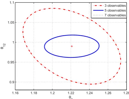
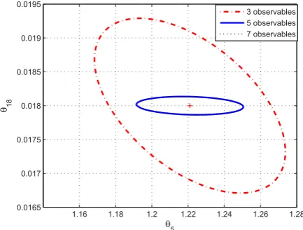
Since the result of parameter estimation highly relies on the efficiency of the optimisation algorithm, it is perhaps not the best way to evaluate the effects of measurement set se-lection. Confidence interval, instead, is a more reliable as-sessment regarding each design and is worked out from the FIM following Cramer-Rao inequality. In general, a smaller confidence interval indicates an estimation with less errors, and vice versa. For the first 3 experiments, the corresponding 95%confidence interval of several parameter pairs are illus-trated in Fig. 1 to Fig. 4, in which+stands for the nominal value of the parameters. Two parameters are chosen in each figure just to present the results in a 2D plane.
1.16 1.18 1.2 1.22 1.24 1.26 1.28
0.9 0.95 1 1.05 1.1
θ5
θ12
3 observables 5 observables 7 observables
Fig. 1: Confidence interval of parametersθ5andθ12
[image:4.595.314.528.478.642.2]min-1.16 1.18 1.2 1.22 1.24 1.26 1.28 0.016
0.0162 0.0164 0.0166 0.0168 0.017 0.0172 0.0174 0.0176
θ5
θ13
[image:5.595.52.267.67.230.2]3 observables 5 observables 7 observables
Fig. 2: Confidence interval of parametersθ5andθ13
1.16 1.18 1.2 1.22 1.24 1.26 1.28
0.22 0.23 0.24 0.25 0.26 0.27 0.28
θ5
θ16
[image:5.595.318.528.234.399.2]3 observables 5 observables 7 observables
Fig. 3: Confidence interval of parametersθ5andθ16
1.16 1.18 1.2 1.22 1.24 1.26 1.28
0.0165 0.017 0.0175 0.018 0.0185 0.019 0.0195
θ5
θ18
3 observables 5 observables 7 observables
Fig. 4: Confidence interval of parametersθ5andθ18
imum number of states to be measured, the estimation ac-curacy could be poor even when the most informative state variables are selected. Certain information about the un-known parameters setθ are missing when using less than necessary measurements. On the other hand, the estimation
results won’t improve much when more than necessary mea-surements are taken into calculation. This is also validated by the parameter estimation results in Table 1.
When selecting measurement set, it is also important to take the more informative observables rather than those con-taining less information. By comparing the confidence inter-val ellipsoids in Fig. 5, it can be clearly seen that the confi-dence interval using the 5 optimal observables (top 5 states inX∗) is much smaller than the one using 5 non-optimal ob-servables (bottom 5 states inX∗). The former has a smaller parameter estimation error owing to the fact that the selected measurement set contains more information about the un-known parameters.
1 1.1 1.2 1.3 1.4 1.5
0.6 0.8 1 1.2 1.4 1.6
θ5
θ12
optimal observables non−optimal observables
Fig. 5: Comparison of confidence interval of parametersθ5
andθ12w.r.t. the optimal and non-optimal observables
5
Conclusions and Discussions
[image:5.595.56.269.285.449.2] [image:5.595.52.269.505.669.2]evalu-ate and apprecievalu-ate feasibility and efforts required in exper-iments, on the other hand, experimental scientists develop a better understanding on which kind of information is most helpful to model development.
Acknowledgement
We would like to thank Dr. Taiyuan Liu for the helpful discussions and aid in programming, also thank Dr. Fei He for helping with the programming of experimental design and confidence interval output.
Appendix
The model presented here is a simplified version of the NF-κB signal pathway model [17] with IκBβ and IκBε
knock out. The reaction species and state variable definition is given in Table 2, in which the subscript ’-t’ represents the mRNA corresponding to the former protein and ’n’ indicates the proteins inside nucleus. The values of model parameters are listed in Table 3 with units ofμM for concentration and minute for time. The constant term Source is taken to be 1μM in ODEs.
Table 2: IκB-NF-κB Model States States Species States Species
x1 IκBα x6 IKK
x2 NF-κB x7 NF-κBn
x3 IκBα-NF-κB x8 IκBαn
x4 IKKIκBα x9 IκBαn-NF-κBn
[image:6.595.50.291.574.782.2]x5 IKKIκBα-NF-κB x10 IκBα−t
Table 3: IκB-NF-κB Model Parameter Values
θ1 30 θ9 30 θ17 0.00678
θ2 6e-5 θ10 6e-5 θ18 0.018
θ3 30 θ11 9.24e-5 θ19 0.012
θ4 6e-5 θ12 0.99 θ20 11.1
θ5 1.221 θ13 0.0168 θ21 0.075
θ6 6e-5 θ14 1.35 θ22 0.828
θ7 5.4 θ15 0.075 θ23 0.0072
θ8 0.0048 θ16 0.2448 θ24 0.2442
A set of ordinary differential equations are used to de-scribe the system dynamics.
˙
x1 = (θ17+θ18)x1+θ2x3+θ15x4+θ19x8+θ16x10
−θ1x1x2−θ14x1x6
˙
x2 = −θ7x2+ (θ2+θ6)x3+ (θ4+θ5)x5+θ8x7
−θ1x1x2−θ3x2x4
˙
x3 = −(θ2+θ6)x3+θ21x5+θ22x9+θ1x1x2
−θ20x3x6
˙
x4 = −(θ15+θ24)x4+θ4x5+θ14x1x6−θ3x2x4
˙
x5 = −(θ4+θ5+θ21)x5+θ3x2x4+θ20x3x6
˙
x6 = (θ15+θ24)x4+ (θ5+θ21)x5−θ23x6−θ14x1x6
−θ20x3x6
˙
x7 = θ7x2−θ8x7+θ10x9−θ9x7x8
˙
x8 = θ18x1−θ19x8+θ10x9−θ9x7x8
˙
x9 = −(θ10+θ22)x9+θ9x7x8
˙
x10 = θ11Source−θ13x10+θ12x27
References
[1] E.O. Voit, Computational Analysis of Biochemical Systems. Cambridge, UK: Cambridge University Press, 2000.
[2] A.C. Atkinson, A.N. Donev, and R. Tobias,Optimum Experi-mental Designs, with SAS, Oxford University Press, 2007. [3] D.C. Montomery,Design and Analysis of Experiments, 5th ed.
New York: John Wiley, 2001.
[4] P.E. Box, J.S. Hunter, and W.G. Hunter,Statistics for Experi-menters: Design, Innovation, and Discovery, 2nd ed. New Jer-sey: Wiley Insterscience, 2005.
[5] K. Chaloner and I. Verdinelli, Bayesian experimental design: a review,Statist. Sci., 10(3): 273-304, 1995.
[6] L. Pronzato, Optimal experimental design and some related control problems,Automatica, 44(2): 303-325, 2008. [7] G. Franceschini and S. Macchietto, Model-based design of
ex-periments for parameter precision: State of the art,Chemical Engineering Science, 63(19): 4846-4872, 2008.
[8] C. Kreutz and J. Timmer, Systems biology: experimental de-sign,FEBS Journal, 276(4): 923-942, 2009.
[9] L. Ljung,System Identification: Theory for the User. Engle-wood Cliffs, NJ: Prentice Hall, 1999.
[10] S. Audoly, G. Bellu, L. DAngio, M.P. Saccomani and C. Co-belli, Global identifiability of nonlinear models of biological systems,IEEE Trans. on Biomedical Engineering, 48(1): 55-65, 2001.
[11] M. Rodriguez-Fernandez, P. Mendes, and J.R. Banga, A hy-brid approach for efficient and robust parameter estimation in biochemical pathways,BioSystems, 83(2-3): 248-265, 2006. [12] H. Yue, M. Brown, F. He, J.F. Jia and D.B. Kell, Sensitivity
analysis and robust experimental design of a signal transduc-tion pathway system,International Journal of Chemical Kinet-ics, 40(11): 730-741, 2008.
[13] F. He, M. Brown, and H. Yue, Maximin and Bayesian robust experimental design for measurement set selection in mod-elling biochemical regulatory systems, International Journal of Robust and Nonlinear Control, 24(6): 1059-1078, 2010. [14] S. Boyd and L. Vandenberghe,Convex Optimization,
Cam-bridge University Press, 2004
[15] P. Flaherty, M.I. Jordan, and A.P. Arkin, Robust design of bi-ological experiments, inProc. of the Neural Information Pro-cessing Systems (NIPS), Cambridge, USA, 2006: 363-370. [16] N.D. Perkins, Integrating cell-signalling pathways with
NF-κB and IKK function,Nature Reviews Molecular Cell Biology, 8(1): 49-62, 2007.
[17] A. Hoffmann, A. Levchenko, M.L. Scott and D. Baltimore, The IκB-NF-κB signaling module: temporal control and se-lective gene activation,Science, 298, 1241-1245, 2002. [18] D.E. Nelson, A.E.C. Ihekwaba, M. Elliott, J. Johnson,
C.A. Gibney, B.E. Foreman, G. Nelson, V. See, C.A. Horton, D.G. Spiller, S.W. Edwards, H.P. McDowell, J.F. Unitt, E. Sul-livan, R. Grimley, N. Benson, D. Broomhead, D.B. Kell, and M.R.H. White, Oscillations in NF-κB signaling control the dy-namics of gene expression,Science, 306: 704-708, 2004. [19] T. Lipniacki, P. Paszek, A.R. Brasier, B. Luxon, and M.
Kim-mel, Mathematical model of NF-κB regulatory module, Jour-nal of Theoretical Biology, 228(2):195-215, 2004.
[20] L. Ashall, C.A. Horton, D.E. Nelson, P. Paszek, C.V. Harper, K. Sillitoe, S. Ryan, D.G. Spiller, J.F. Unitt, D.S. Broom-head, D.B. Kell, D.A. Rand, V. S´ee, and M.R.H. White, Pul-satile stimulation determines timing and specificity of NF-κ B-dependent transcription,Science, 324(5924), 242-246, 2009. [21] Y.S. Jin, H. Yue, M. Brown, Y. Liang, and D.B. Kell,