Survey of classical density functionals for modelling hydrogen physisorption at 77 K

Survey of classical density functionals for modelling hydrogen physisorption at 77 K

Department of Chemical and Process Engineering, University of Strathclyde, Glasgow, G1 1XJ, United Kingdom

共Received 30 November 2007; published 28 February 2008兲

This work surveys techniques based on classical density functionals for modeling the quantum dispersion of physisorbed hydrogen at 77 K. Two such techniques are examined in detail. The first is based on the “open ring approximation”共ORA兲 of Broukhno et al., and it is compared with a technique based on the semiclassical approximation of Feynman and Hibbs共FH兲. For both techniques, a standard classical density functional is used to model hydrogen molecule–hydrogen molecule共i.e., excess兲interactions. The three-dimensional共3D兲 quan-tum harmonic oscillator共QHO兲system and a model of molecular hydrogen adsorption into a graphitic slit pore at 77 K are used as benchmarks. Density functional results are compared with path-integral Monte Carlo simulations and with exact solutions for the 3D QHO system. It is found that neither of the density functional treatments are entirely satisfactory. However, for hydrogen physisorption studies at 77 K the ORA based technique is generally superior to the FH based technique due to a fortunate cancellation of errors in the density functionals used. But, if more accurate excess functionals are used, the FH technique would be superior. DOI:10.1103/PhysRevE.77.026712

I. INTRODUCTION

The path-integral共PI兲formulation of quantum mechanics 关1兴allows equilibrium quantum particles to be represented as unusual classical ring polymers. This mapping converges to the exact quantum mechanical result in the limit thatn, the number of sites on a single ring-polymer ring, tends to infin-ity. This ring-polymer representation is very convenient and invites关2,3兴the techniques of classical statistical mechanics to be used to solve some quantum problems.

Path integral simulations, both Monte Carlo共PI-MC兲and molecular dynamics共PI-MD兲, are popular in this context and provide accurate information that are in principle exact共to within statistical error兲for a givenn. But these methods can be computationally demanding, especially for large n. So, theoretical alternatives to simulation are often useful. In the field of classical fluids density functional theory共DFT兲is a powerful tool with a wide range of applications, including simple fluids, polymers, colloids, etc. For situations with sig-nificant symmetry, for example those involving spherical particles adsorbed into slit or cylindrical pores, etc., DFT calculations can be up to several orders of magnitude more efficient, sometimes without significant loss of accuracy, compared to simulation. Hard spheres in slit pores are a good example here; hard-sphere DFTs are often solved in a few seconds on a desktop PC, whereas corresponding MC simu-lations might take several minutes to obtain a satisfactory level of precision. Path-integral simulations are more de-manding still. So DFT is an attractive technique, not only for gaining fundamental theoretical understanding, where abso-lute accuracy is not essential, but also for engineering appli-cations共optimization studies, for example兲where calculation efficiency must be weighed against accuracy.

Consequently, in recent years, several studies have at-tempted to apply the classical version of density functional theory to model quantum particles via the PI–classical ring-polymer mapping关3兴, resulting in several approximate path-integral density functional theories 共PI-DFTs兲. The aim of these studies is to develop finite-temperature DFT techniques

that, for situations where the symmetries mentioned above allow, are significantly more efficient than the corresponding Monte Carlo approach. They require the development of classical density functionals for these unusual ring polymers. For example, Broukhno et al. 关4兴 recently developed a PI-DFT based on what they call the “open ring approxima-tion”共ORA兲, which equates any site in a ring polymer with the middle site in the corresponding chain polymer. The chain-polymer problem is then easily solved exactly using the propagator approach of Woodward关5兴, which is also de-scribed below. They claim that their approximation becomes exact in the same limit that the PI technique becomes exact, i.e., n_→⬁, and validate their method by comparison with exact results for some simple spherically symmetric systems, including the 3D quantum harmonic oscillator 共QHO兲 and the ground state of the hydrogen atom. They claim that their excellent results validate the ORA. Their results are impres-sive, if taken at face value, and suggest that their PI-DFT could find wide application. However, in fact the ORA is flawed and produces the wrong limit as n_→⬁. In other words, the statistics of ring and chain polymers are not equivalent in this limit. This result has been known for a long time 关6,7兴. Their technique is described below 共in its cor-rected form兲and their results for the 3D QHO are confirmed. It is also shown how this ORA technique, and indeed any PI-DFT technique based on classical density functionals for ring polymers, can be extended to model adsorption in the grand canonical ensemble. Results for the hydrogen adsorp-tion problem demonstrate that the ORA is not generally ac-curate.

actual density profiles were not derived or shown. The work described below is the first example where the FH approxi-mation is combined with a classical DFT for nonuniform fluids 共which is used to model “excess” interactions, i.e., hydrogen molecule–hydrogen molecule interactions兲, and it is shown how density profiles that include dispersion can be obtained. It is found that the FH technique performs well for low density physisorption of molecular hydrogen on a gra-phitic surface, although the mean-field density functional used to model excess interactions introduces some error at higher densities.

The work of Broukhnoet al.is not the first application of classical ring-polymer density functionals to this problem. Guet al.关11兴also developed a density functional theory for ring polymers, this time based on a particular version关12兴of “statistical associating fluid theory”共SAFT兲 that deals with ring polymers. However, because SAFT is a perturbation theory their ring-polymer model does not correspond to the PI–ring-polymer mapping. Their model consists of hard-sphere sites joined together to form a ring. Interactions be-tween hard-sphere sites are allowed both within a single ring polymer and between all sites on different ring polymers. In a PI ring polymer interactions within a ring polymer should be limited to harmonic bonds between adjacent sites, and only sites with the same index共or label兲 interact with each other on different ring polymers. These are very different ring polymer models. No attempt is made to describe their method or reproduce their results here, but comparison is made between the results of the techniques examined in this work and their published results. It is found that their work is seriously flawed. Not only does their PI–DFT not correspond to the PI—ring-polymer mapping, but their grand canonical PI-MC simulation results, which they used to validate their theory, are also found to be qualitatively incorrect.

Note that the first关13兴density functional theory for non-uniform ring polymers was based on a weighted density ap-proximation 共WDA兲 for bonding. In that work it was sug-gested that this ring-polymer DFT could be adapted to model quantum dispersion. Although this turns out to be true关14兴, this approach also suffers a serious problem. The problem is that this particular DFT for ring polymers is approximate, and so it does not generate results that converge to a limit as n→⬁. In a sense this is worse than the ORA of Broukhnoet al., which only converges to the wrong limit. By fine-tuning nin this technique it is possible to calibrate this WDA-based PI-DFT, but the calibration process is inconvenient and re-sults produced by this method do not offer any significant advantage over the Feynman-Hibbs based method for hydro-gen physisorption on a graphitic surface at 77 K. Conse-quently, it is not presented here.

Finally, path-integral Monte Carlo 共PI-MC兲 simulation, both its canonical and grand-canonical versions, is used as a benchmark to test the density functionals for the hydrogen adsorption problem. This PI-MC algorithm is itself validated by comparison with exact results for the 3D-QHO system.

Two tests are employed in this work to compare the tech-niques described above. One test is a system consisting of single quantum particle in a 3D harmonic oscillator at finite temperature, for which exact results are easily obtained共see Appendix A兲. The second is a model of hydrogen adsorption

in graphitic slit pores at 77 K. At this temperature the ther-mal de Broglie wavelength of molecular hydrogen is 0.14 nm, which is more than twice the lengthscale of the hydrogen-graphite interaction共⬃0.06 nm兲but less than half the average interparticle separation at the highest hydrogen densities considered in this work 共⬃0.34 nm兲. This means that quantum effects should be significant with respect to the hydrogen-graphite interaction but they should not be signifi-cant with respect to hydrogen-hydrogen interactions. In other words, molecular hydrogen at 77 K adsorbed onto graphitic surfaces will exhibit significant quantum dispersion but not significant quantum exchange, and so presents a suitable test case for the DFT techniques presented here. Moreover, stud-ies of molecular hydrogen physisorption have received a great deal of attention, particularly over the last decade or so, in line with research into the “hydrogen economy” and espe-cially hydrogen storage 关15兴. It is known that significant quantities of hydrogen, at either elevated pressure or reduced temperature 共or both兲 关16兴, can be stored when physisorbed in microporous materials. But to discover an optimal adsor-bent material together with optimal conditions of tempera-ture and pressure is a challenge that still consumes a great deal of effort关17兴.

One of the difficulties in this respect is the quantum na-ture of hydrogen at low temperana-ture. A range of techniques have been used to model these quantum effects, from PI-MC simulations关18,19兴to more efficient approximate techniques based on the Feynman-Hibbs共FH兲approach combined with Monte Carlo or molecular dynamics simulations. Stan and Cole 关20兴 also used the FH approach to model hydrogen adsorption, but only considered the low density limit where excess interactions are absent, while Kowalczyk and MacEl-roy 关21兴 combined the FH technique with a standard DFT describing excess interactions but only considered the bulk limit. Gu et al. 关11兴 developed the first PI-DFT technique based on classical density functionals for nonuniform fluids, although as described earlier, their method is flawed. So the work described below is the first serious attempt to model the quantum dispersion of hydrogen adsorption at 77 K us-ing only techniques based on classical density functionals.

The remainder of this paper is structured as follows. The theory section briefly describes each of the techniques above. The test systems are described in detail, and results for these test systems are presented and compared for each technique. The paper is concluded with a discussion.

II. THEORY

with an external field,Vext_{, but only with 1/nth the strength}

of the original potential. In the absence of exchange interac-tions these ring-polymers particles obey classical Boltzmann statistics, so for N identical “Boltzmannons” the partition function is

Q= 1 N!

冉

n␤␭

␲

冊

3Nn/2

冕

⫻exp关−␤共Hintra+Hinter+Hext兲兴, 共1兲 where the intrapolymer, interpolymer, and external potential contributions to the Hamiltonian are, respectively,

Hintra=

兺

i=1 N

Hintra共Ri兲=n␭

兺

兺

j=1 n

r_ij2_·ij+1, 共2兲

Hinter=1 n

兺

兺

n

␾共rik·jk兲, 共3兲

Hext=

兺

i=1 N

Hext共Ri兲=

1 n

兺

N

兺

j=1 n

Vext共rij兲. 共4兲

Here, 2n␭=mn/共_␤ប兲2 _{is the “spring constant” of the} in-tramolecular interactions,ប is Planck’s constant divided by 2␲,␤= 1/kBT 共whereT is the temperature兲, mis the

parti-cle’s mass,Ri=兵ri1,ri2,. . . ,rin其 is the set of coordinates for

the sites of theith ring polymer,rik·jl=兩rik−rjl兩is the

separa-tion between thekth site on the ith ring polymer and thelth site on thejth ring polymer, andr_in+1=r_i1to create the rings. Essentially, the total interparticle and external potential inter-action energies are averaged over the path of the ring poly-mer. This path is, for an isolated ring polymer, rather like a random 3D walk of steps with a range of lengths consistent with the intramolecular springlike bonds共it is not a perfectly random path because the final site is adjacent to the first兲. Note the thermal de Broglie wavelength⌳=

冑

Following Woodward 关5兴, the exact Helmholtz free en-ergy for the system of PI ring polymers is expressed in terms of thering polymerdensity␳共R兲,

F=Fid+Fb+Fext+Fex

=k_BT

冕

␳共R兲兴− 1其

+

冕

冕

whereVintraandVextare the intramolecular and external po-tentials for a single ring polymer关obtained by settingN= 1 in Eqs.共2兲and共4兲兴. Here, the first term is the ideal contribution for a gas consisting of molecules which are formed fromn sites each, the second term accounts for the harmonic bonds between adjacent sites on each ring polymer and bonds the appropriate sites together to form a ring, the third term ac-counts for the interaction with the external potential, while the last “excess” term describes interactions between differ-ent ring polymers. Although an elegant formulation, the problem with this approach is the description of a ring

poly-mer in terms ofR, which can have very many dimensions. An alternative representation of this system can be ob-tained based on the interaction-site density functional for-malism of Chandleret al.关22,23兴. Here, the exact Helmholtz free energy density functional is written in terms of the total site density␳s共r兲,

F=Fid+Fext+Fb+Fex

=kBT

冕

/2_␳

s共r兲兴− 1其

+1

n

冕

ext_共r兲

+Fb+Fex. 共6兲

Once again, the first term on the right is the ideal gas con-tribution, the next term accounts for the interaction with an external potential, the third term accounts for bonded inter-actions, and the last term describes all other interactions. The advantage of this description is that, becauserhas far fewer dimensions thanR, techniques based on it could potentially be as efficient as DFTs for simple fluids 共which area also described in terms ofr兲. However, contrary to the Woodward

approach, with this interaction-site approach an exact and compact expression is lacking for the bonding functional. This is a serious disadvantage because for the ring-polymer—PI mapping we prefer the ring-polymer density functional to converge to a fixed limit, close to the exact limit, asn→⬁. Yet, because any bonding functional is nec-essarily approximate with this approach, this is not guaran-teed. So PI-DFT techniques based on this approach could suffer serious problems, like the WDA-based method men-tioned earlier.

A. Open ring approximation

Broukhnoet al.explain that an exact solution of the ideal 共i.e., ignoring the excess functional Fex_{兲 PI ring-polymer}

problem corresponding to Eq.共5兲can be achieved but only at considerable computational expense. The difficulty, com-pared to chain polymers, arises because of the need to ensure that the polymer forms a ring, which requires one to keep track of where the “beginning” and “end” points of a ring are. In the general case this presents severe computational difficulties, although for systems with reduced symmetry, such as fluids with spherical particles adsorbed on planar surfaces, calculations should be much less demanding. Be-cause of this, Brouknoet al. are able to solve the exact PI ring-polymer problem for a single particle in a 1D-QHO quite straightforwardly.

␳_smid共r兲= exp兵−␤关Vext共r兲/n−␮兴其关G_共n−1兲/2 lin

共r兲兴2, 共7兲

where the propagators,G_jlin共r兲, for freely jointed chains are

given by

G_jlin共r1兲=

冕

共r2兲exp关−␤Vext共r2兲/n兴

⫻exp共−n␤␭r12 2 _{兲, j}

⬎0,

G0 lin_共r

1兲= 1. 共8兲

Here,␮is the Lagrange multiplier that achieves the correct total number of middle-sites共which becomes the configura-tional contribution to the chemical potential in the grand ca-nonical ensemble兲. Note that in their work关4兴 Broukhnoet al.use the index “n/_{2” in Eq.}共7兲_{and consider polymers with} an even number of sites, instead of the index “共n− 1兲/_{2” and} polymers with an odd number of sites. It follows that the external potential in their work is too large by a factor of 共1 +n−1_{兲. This will reduce the rate of convergence asn}

→⬁ in their work, and explains why large values ofnare needed in their work even for high temperatures. For nonideal ring polymers共where the excess functionalFex⫽0兲, the external

potential Vext_{共r兲 in Eqs. 共7兲 and 共8兲 is replaced by V}ext_共r兲

+␦Fex_{/␦␳共r兲, where ␳共r兲=␳} s

mid_{共r兲. This excess functional is}

defined later.

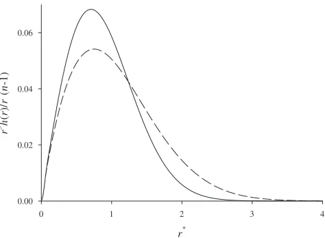
However, contrary to their claims, the ORA does not be-come exact in the limit n_→⬁. It is well known that the statistics of fully flexible noninteracting ring and chain poly-mers are very different 关6,7兴, and in the n_→⬁ limit the squared radius of gyration for a ring polymer is half that of a chain polymer. Because the density profile of the middle site in a chain polymer is influenced by the distribution of the other sites in the same polymer, this implies that it cannot be equivalent to the density profile of a site in a ring polymer. One can also compare the total intrapolymer site-site pair correlation function for the middle site in a chain polymer and any site in the corresponding ring polymer in the n →⬁ limit for a bulk situation. Figure 1 clearly shows that these polymers are quite different 共see Appendix B for a derivation of the equations depicted in Fig. 1兲. This figure compares these functions for n= 1001, which is sufficiently large that no visible difference is observed on the scale of this plot when n is increased further. The ring polymer is much more compact than the chain polymer. This means that we should expect the chain polymer to underpredict the true density profile of a quantum system in the grand canonical ensemble because it will tend to generate too much smooth-ing due to dispersion. The effect for a canonical ensemble system will be more subtle because the total number of par-ticles is fixed. However, we still should expect it to produce a smoother, more dispersed, density profile.

So in general we should not expect the ORA to be accu-rate. Yet in their work, Broukhnoet al. showed that it was extremely accurate for some particular spherically symmetric external potentials, namely the 3D-QHO and for the electron density surrounding some atomic nuclei. They claim that this

level of accuracy should also be seen more generally. One of the aims of this present work is to show that this is not the case.

B. Feynman-Hibbs technique

In this approach a quantum particle is approximated by a three-dimensional Gaussian wave packet which is used to calculate effective interactions between the quantum particle and other particles. It is a well-known technique that is de-scribed in detail elsewhere关1,24,25兴. The effective potential is

V_cleff共r1兲=共2␲⌬q2兲−3

/2

冕

2Vcl共r2兲exp共−r12 2 _/

2⌬q2_兲

, 共9兲

where ⌬q2_=␤ប2_/12m=k

BT/24␭, r12=兩r1−r2兩, Vcl is the

“bare” classical potential, and the mass m is the reduced mass of the quantum particle and the object it is interacting with. Although it is straightforward to evaluate this integral precisely numerically, for some of the divergent potentials used in this work it should approximated by performing a Taylor series expansion of the interaction potentialVclabout

r1. For the effective interaction between two spherical

quan-tum particles the result to second order in the series expan-sion is

␾eff_{共r兲=␾共r兲+}

冉

24m

冊

2_␾共r兲

=␾共r兲+

冉

2

12m

冊冉

⳵2␾共r兲

⳵_r2 +

2 r

⳵␾共r兲

⳵_r

冊

whereris their separation andmis the mass of one particle. For the effective interaction between a quantum particle and an immobile spherically symmetric external potential the corresponding result is

r*

0 1 2 3 4

r

3 h

(

r

)/

r

* (

n

-1)

0.00 0.02 0.04 0.06

FIG. 1. Comparison of the normalized total site-site intramo-lecular correlation function for fully flexible noninteracting chain

V_exteff共r兲=Vext共r兲+

冉

2

24m

冊

2_Vext_共r兲

=Vext共r兲+

冉

2

24m

冊冉

⳵2Vext共r兲

⳵_r2 +

2 r

⳵_Vext_共r兲 ⳵_r

冊

共11兲

For the effective interaction between a quantum particle and an immobile planar surface the result is

V_exteff共z兲=Vext共z兲+

冉

2

24m

冊

⳵2Vext共z兲

⳵z2 , 共12兲

wherezis the distance normal to the surface. These effective interaction potentials can be combined with DFT for classi-cal fluids to arrive at an Euler-Lagrange equation for the density profile of the effective classical particles,

␳eff_共r

1兲= exp

冋

冉

r1兲−␮+

␦Fex

␦␳eff_共r 1兲

冊

册

, 共13兲

where ␮ is the Lagrange multiplier 共or configurational chemical potential for the grand canonical ensemble兲andFex

is an excess Helmholtz free-energy density functional for a system described in terms of effective interactions, ␾eff

. These interactions and the correspondingFex_{are described in}

the next section. To obtain the actual density profile includ-ing the effect of quantum dispersion the effective density profile must be convoluted with the 3D wavepacket once more. So we have

␳共r1兲=共2␲⌬q2兲−3

/2

冕

2␳eff共r2兲exp共−r12 2

/_2⌬q2兲.

共14兲

This technique is denoted FH-DFT.

C. Excess functional

Each of the techniques described above requires a pre-scription for the excess functional. In this work an excess functional is only needed for the hydrogen physisorption problem since the 3D QHO test only involves a single par-ticle. If our system comprises only ring polymers represent-ing hydrogen molecules, and if we label the sites on each ring polymer 1 . . .n and consider the system to consist of a mixture of sites, i.e., if we adopt the interaction-site model of Chandleret al.关22,23兴 共6兲, then the excess functional for a grand canonical ensemble can be written using the well-known density functional relation关26兴

Fex=kBT

兺

冕

d␣共␣− 1兲

冕

冕

⫻c_ij共2_,ex兲 共r1,r2,␳␣兲, 共15兲 wherec_ij共2_,ex兲 共r₁,r₂,␳␣兲 is the “excess” pair-direct correlation function acting between sites i and j for the system with density ␳␣=␣␳共r兲 and ␳i共r兲 is the density of sites labeled

i. This excess function is simply the total site-site pair-direct correlation function less the contribution due to the

bonding functional c_ij共2_,ex兲 共r1,r2兲=cij 共2兲_共

r1,r2兲−cij,b 共2兲_共

r1,r2兲,

where c_ij共2_,兲_b共r1,r2兲= −␤␦2Fb/␦␳i共r1兲␦␳j共r2兲. Because of the

symmetry of the ring and because each site is identical 共ex-cept for its label兲, Eq.共15兲can be written

Fex=kBT

冕

1

d␣共␣− 1兲

冕

冕

1,r2,␳␣兲, 共16兲

wherec_n共2兲=n兺j=1,nc1j,ex 共2兲

. Because there are no site labels in Eq.共16兲, it has the same form as a density functional theory for a simple classical system interacting via an effective ring-polymer–ring-polymer interaction that generates the pair-direct correlation function c_n共2兲. The Feynman-Hibbs tech-nique prescribes an approximation for this effective interaction via Eq.共10兲. But in general we are free to choose the effective interaction so that it generates these pair corre-lations accurately. Density functionals able to model these effective interactions are discussed below. As mentioned ear-lier in the context of the ORA technique, the external poten-tial, Vext_{共r兲, in Eqs. 共7兲 and 共8兲 should be replaced with}

Vext共r兲+␦Fex/_␦␳共r兲, whereFexis given by Eq.共16兲. We de-note this technique ORA-DFT. But de-note that the derivation of Fexhere is quite general, and not limited to the ORA-based method.

In this work molecular hydrogen is modeled as a single quantum particle and the distinction between ortho- and parahydrogen is not made. This model is thought to be suf-ficient at the temperatures considered in this work. So, for both the FH-DFT and ORA-DFT techniques we must define an excess functional corresponding to a model of effective H2-H2 interactions. In this work all such effective

interac-tions are described by Lennard-Jones 共LJ兲 interactions and hence standard excess functionals that describe LJ fluids are used. Although the FH technique actually prescribes a slightly different effective interaction, this effective FH in-teraction is accurately modelled by a LJ inin-teraction共see the Results section兲. So a standard approximate DFT expression for LJ fluids is used

Fex关␳共r兲兴=F_dex关␳共r兲兴+1

2

冕

冕

whereF_dex is the original fundamental measure hard-sphere functional of Rosenfeld 关27兴 and of Kierlik and Rosinberg 关28,29兴, and ␾att is the attractive contribution to LJ

interac-tion. The hard-sphere diameterdis set equal to the LJ length parameter␴eff_{, while␾}

attis determined according to the

pre-scription of Weeks, Chandler, and Andersen共WCA兲 关30兴 ap-plied to a cut-and-shifted LJ potential

␾att共r兲=

冦

−␧eff

−␾LJ共rc兲, r艋21

/6_␴eff

,

␾LJ共r兲−␾LJ共rc兲, 21

/6_␴eff_⬍r艋r c,

0, r⬎rc,

冧

共18兲

␾_LJ共r兲= 4␧eff共x−12−x−6兲, 共19兲 x=r/␴eff_{, andr}

cis the cutoff radius共equal to 1.5 nm in this

work兲. These functionals are well known and described else-where in detail关26兴. Application to slit pores is straightfor-ward关31,32兴. Although other potentials thought to be more accurate have been used to model molecular hydrogen in other work they are not used here for several reasons. First, the focus of this work is not actually the precise prediction of hydrogen adsorption, but instead the comparison of several techniques capable of modelling hydrogen adsorption effi-ciently. On this basis alone there is no need to use models that might offer slightly greater accuracy than the LJ model, which is adequate for the purpose of this work. Secondly, it is likely that the approximation共17兲, which could be applied straightforwardly to other potentials if required to do so, gen-erates greater error than choosing the LJ potential over other possibly more accurate potentials. In any case, we will see below that the LJ potential and Eq.共17兲is able to accurately reproduce a bulk isotherm of hydrogen at 77 K.

As mentioned above, this excess density functional pre-scription for LJ fluids is known关33,34兴to be only reasonably accurate for modelling adsorbed fluids, even if the model parameters are chosen to accurately reproduce bulk data. Much greater accuracy can often be achieved关33,34兴 with more sophisticated共and somewhat more demanding兲density functionals for LJ fluids.

Both the FH-DFT and ORA-DFT techniques are solved by Picard iteration. The excess density functional is given in each case by Eq.共17兲, but the effective Lennard-Jones pa-rameters that enter this functional are different in the FH-DFT and ORA-FH-DFT approaches and determined later.

D. PI-MC simulations

The techniques described above based on classical density functionals are compared to results generated by PI-MC. Ca-nonical ensemble PI-MC simulation is used for the 3D-QHO test, while the grand canonical PI-MC technique共PI-GCMC兲 used in this work to model hydrogen adsorption is similar to that introduced by Wang and Johnson关35兴. The only signifi-cant difference with their work is that a hybrid MD technique is not used to perform a displacement move. Instead, a more straightforward Monte Carlo scheme is used. In this scheme a trial displacement consists of moving a single ring-polymer as follows. Each site on the ring-polymer is moved by the same amountdr0共chosen randomly with uniform probability

from within a sphere of radiusdr0兲, and then each site is also

moved an additional dr_i 共chosen randomly with uniform

probability within a sphere with radius dr1兲, where dri is

different for each site i. dr1⬍dr0 must be quite small to

ensure a reasonable probability of acceptance 共generally about 50%兲. For each simulation 5.12 million trial moves are attempted, half of which are attempted displacement moves 共the other half are trial insertions and deletions兲, with an additional 0.5 million attempts to allow equilibration. 100 noninteracting “gas-phase” PI ring polymers are simulated simultaneously to provide a pool of random configurations that can be used to generate trial insertions. This PI-GCMC technique is compared with exact results for the 3D QHO to

determine the largest value ofnfor which it is ergodic for the kinds of systems studied here. Results are presented later.

E. Test systems

The 3D QHO system is studied to confirm the results of Broukhnoet al.for the ORA and to validate the PI-GCMC algorithm used here. A 3D harmonic oscillator is defined by the potential

Vext共r兲=1 2Kr

2

, 共20兲

whereK is the spring constant. We consider a single quan-tum particle system at fixed temperature, i.e., a canonical ensemble. The exact solution for energy levels and density profiles of the 3D QHO is given in Appendix A. From this solution we see that only two independent parameters are needed to define a 3D QHO: An inverse length

␥=

冑

冑Km

and the dimensionless parameter

␦=ប

冑K

k_BT , 共22兲

which is related to the probability that the system is in its ground state,p共0兲=关2e−␦/2_{sinh共␦/2兲兴}3_{. So, by working with}

a reduced length,r*₌r␥, we have to consider only one pa-rameter,␦. Because of the spherical symmetry of this poten-tial numerical solutions are most conveniently found using fast Fourier transforms关31兴.

The main part of this paper studies hydrogen physisorp-tion at low temperature. For this problem the bare, or high temperature, hydrogen molecule–hydrogen molecule interac-tion 共i.e., not the effective hydrogen molecule–hydrogen molecule interaction兲is set equal to that used in other work 关11兴. That is, a molecular hydrogen site is modeled as a Lennard-Jones particle with energy and length parameters equal to ␧ff/kB= 36.7 and ␴ff= 0.296 nm, respectively. As

usual, a slit-pore is defined as two parallel ideal walls sepa-rated by a distanceH

Vext共z兲=Vst共z兲+Vst共H−z兲, 共23兲 where the hydrogen molecule–graphitic wall interaction is provided by the Steele potential关31兴

Vst共z兲= 2␲␳s⌬␴sf 2

␧sf

冋

2 5

冉

␴sf

z

冊

10

−

冉

冊

4

− ␴sf

4

3⌬共0.61⌬+z兲3

册

and the Lorentz-Berthelot mixing rules are used to define cross parameters

␴sf=共␴f f+␴ss兲/2, ␧sf=

冑

Surface parameters appropriate for modeling graphite are 关31兴 ␧ss/kB= 28.0 K, ␴ss= 0.34 nm, ␳s= 114 nm−3, and ⌬

III. RESULTS

A. 3D-QHO

Let us consider the Feynman-Hibbs technique applied to the 3D-QHO first. Application of Eqs. 共9兲–共20兲 gives the well-known关24兴result

V_exteff共r兲=Vext共r兲+3K 2 ⌬q

2

. 共26兲

Essentially, the entire potential is shifted by a constant amount. The same result is obtained using the second order version 共11兲. In this system, for which the number of par-ticles is fixed at one, this shift of the potential will have no effect on the density profile of the effective classical par-ticles; it will be exactly the same as the classical result. The effect of quantum dispersion on the density profile is in-cluded through Eq.共14兲, giving the result

␳共r兲=

冉

冊

3/2

e−共␤K␩/2兲r2, 共27兲

where␩=共K⌬q2_{+ 1兲}−1_{. Likewise, the average energy is}

in-creased above the classical energy by 3K⌬q2_{/2. These}

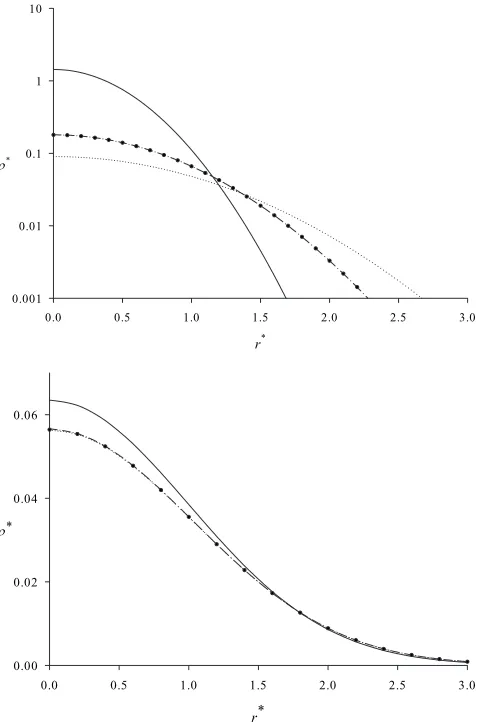
re-sults are displayed in Figs. 2共a兲 and 2共b兲 共density profiles兲 and TableI共energies兲, where they are compared with exact results共A4兲, and results from the ORA. The ORA results of Broukhnoet al.for this system are reproduced, albeit much more efficiently than in their work, due to the use of the correct ORA expression共7兲.

Figure2共a兲compares results for the density profile when

␦= 8 关corresponding to p共0兲= 0.999兴, where r*is described above and␳*=␳/␥3 _{is the reduced particle density with}

re-spect to this reduced length scale. The main plot shows that the ORA performs exceptionally well in this case. Using the ORA, results forn⬃81 and above cannot be distinguished from exact results on the scale of this plot. The FH result significantly “oversmooths” the density profile, which is ex-pected because the Gaussian wave packet employed is fixed in this approximation and cannot adjust to the presence of the external potential.

Figure2共b兲is similar to Fig.2共a兲except that the tempera-ture is higher关␦= 1, corresponding to p共0兲= 0.253兴. Similar comments apply, except now the FH result is much more accurate at this higher temperature. Because the correct ORA expression共7兲 is used in this work it generates satisfactory results even forn= 11, which is several orders of magnitude smaller than typical values in Ref.关4兴.

TableIdisplays the energy for each result shown in Figs. 2共a兲and2共b兲. For each approximate calculation the total en-ergy is determined from the average potential enen-ergy via the virial theorem关36兴, which in this particular case is

2具Ekin典=

冓

⳵_r

冔

Here,Ekin. is the kinetic energy and the angle brackets

de-note an ensemble average. For the classical and FH ap-proachesEkin= 3kBT/2, and hence the total energy is easily

calculated. For the ORA approach the right-hand term in Eq. 共28兲is simply twice the average potential energy. So the total

energy is just twice the average potential energy, which is easily calculated from the density profile. The total energy for the exact result is given in Appendix A. Note that if the energy for each technique had been calculated from the re-sulting approximate wave function and the Schrödinger equation then each result in TableIwould be greater than 1, since 1 indicates the ground state. But this is clearly incorrect for a classical system; hence the use of the virial theorem in FIG. 2. 共a兲 Density profiles for the 3D QHO with ␦= 8. The circles are exact quantum results, while the solid line is the exact classical result. The dot-dash and dottted lines are results from the ORA共withn= 81兲 and the FH methods, respectively. The reduced length and density arer*and␳*, respectively. The reduced density is shown on a logarithmic scale.共b兲As for共a兲except that␦= 1, for the ORA resultn= 11, and reduced density is shown on a linear scale.

TABLE I. The total energy of the 3D-QHO predicted by several methods, expressed relative to the ground-state energy, where␦is given by Eq.共22兲.

␦ Exact ORA FH Classical

8 1.0007 0.9995 0.9167 0.25

this work and in Ref.关4兴which is appropriate for techniques based on ring-polymer models.

Finally, the PI-GCMC algorithm is tested to determine the range ofnover which it is ergodic for␦= 3. This value of␦

is chosen because it produces a similar degree of quantum dispersion to the hydrogen adsorption problem at 77 K, and so is a suitable validation test of the PI-GCMC algorithm used here. The grand-canonical technique is tested using noninteracting quantum particles. An arbitrary chemical po-tential is chosen, and the final density is scaled to achieve an average of 1 particle in the 3D-QHO.

Figure3shows PI-MC results for several values ofn, and compares them against exact classical and quantum results. By inspection, we see thatn艌12 is sufficient for this system, but the technique starts to become nonergodic forn⬎24.

B. Hydrogen physisorption in graphitic pores

Each of the above techniques are compared for a model of hydrogen adsorption in graphitic pores at 77 K, which roughly corresponds to the lower bound of interest in hydro-gen physisorption studies. Pores of 0.7 nm and 2 nm in width are considered because they represent quite different situations. WhenH= 0.7 nm only a single layer of hydrogen is adsorbed, while forH= 2.0 nm we have a layer of hydro-gen on each wall with much more dilute gas filling the re-mainder of the pore.

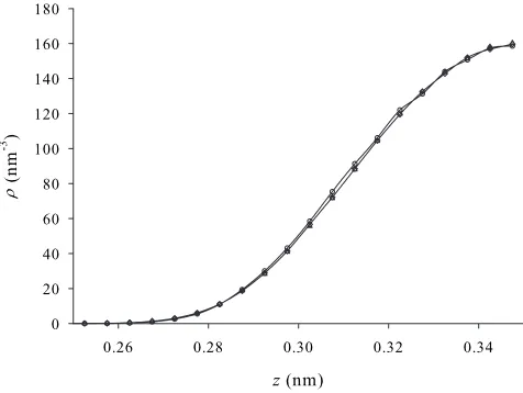
The first task is to determine the lowest value ofn that is sufficient in the PI-GCMC simulations to obtain accurate results. A demanding scenario here is the 0.7 nm pore at the highest activity␰=␳bexp共␤␮ex兲. Figure4displays PI-GCMC

results for several values ofnat 77 K and␰= 1.0 in this pore. We see that increasingnbeyond 8 has little impact relative to

the statistical error in the results. So for all other PI-MC simulations at 77 Knis set to 12, which by comparison with the ␦= 3 3D-QHO results in Fig. 3 is thought to be well within the ergodic regime. Wang and Johnson关18兴find that n= 15 is sufficient in their work at 77 K.

The effective FH potential calculated from Eq. 共11兲 is shown in Fig. 5. For convenience a LJ potential is used in place of the effective FH potential. Figure5also shows this effective FH LJ potential which is determined by finding the closest fit to the second moment of the Mayer function关37兴 共which ensures close agreement in the second virial coeffi-cient兲. So, the effective LJ parameters used for the FH tech-nique are␴eff_{= 0.3076 nm and␧}eff_/k

B= 31.62 K at 77 K.

FIG. 3. PI-GCMC results using the algorithm described in the text for the 3D-QHO with␦= 3 using a range of values ofn:n= 8

共solid triangles with dashed line兲,n= 12共open circles兲,n= 16共open squares兲, n= 20 共open diamonds兲, n= 24 共open triangles兲, and n = 28共solid circles with dashed line兲. The dashed line is the classical result while the solid line is the exact quantum result. The reduced length and density arer*and␳*, respectively. Statistical errors are usually smaller than symbols sizes, except for a few points close to the origin.

FIG. 4. PI-GCMC results for hydrogen adsorption in a 0.7 nm graphitic slit pore at 77 K and␰= 1.0 using a range of values ofn: n= 4 共open circles兲, n= 8 共open diamonds兲, and n= 12 共open tri-angles兲. Lines are a guide to the eye and statistical errors are smaller than symbols sizes. Only a left-hand portion of the pore is shown;zis the distance from the left-hand pore wall.

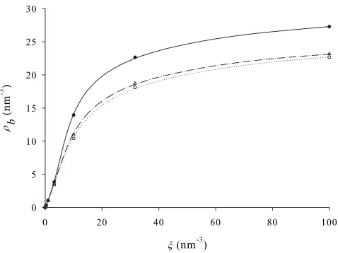
Next, the effective LJ parameters for the FH-DFT and ORA-DFT techniques are determined. For the ORA-DFT technique the effective LJ parameters are optimized to repro-duce bulk hydrogen isotherms generated by PI-MC simula-tions. Here, the aim is to produce the smallest root-mean-square deviation between the bulk isotherm generated by simulation and the bulk isotherm generated by the bulk limit of the DFT. This idea is similar to that used by Kowalczyk and MacElroy 关21兴 in their application to bulk thermody-namics of hydrogen. The best fit DFT parameters to the PI-GCMC results are found to be ␴eff

= 0.2903 nm and ␧eff_/k B

= 28.10 K, while the best fit DFT parameters to GCMC simulations of the LJ potential which is fitted to the FH potential in Figure 5 are ␴eff_{= 0.2908 nm and ␧}eff_/k

B

= 29.60 K. To compare with classical results the same LJ parameter fitting process is used, where this time the best fit is found to classical GCMC simulations results. This gives

␴eff_{= 0.281 nm and␧}eff_/k

B= 34.30 K. Each bulk isotherm is

shown in Fig. 6. All these effective interaction parameters are summarized in TableII. The effective FH external poten-tial corresponding to the interaction of hydrogen with a pore wall is obtained by combining Eqs.共23兲 and共24兲 with Eq. 共12兲.

One advantage of generating effective hydrogen model parameters via this calibration method is that an effective LJ model for hydrogen can be found that compensates, to a degree, for the inaccuracy of the excess functional共17兲. Al-though it could be argued that this method is computationally demanding, because GCMC or PI-GCMC simulations are used to generate the reference bulk isotherms, this would not be the case when using experimental data rather than simu-lation data as a reference, which would normally be the case.

Note that the resulting effective hydrogen–hydrogen LJ in-teraction parameters are quite similar for the FH-DFT and ORA-DFT techniques, and␴eff_{is slightly larger than for the}

corresponding classical parameters, as expected. However, these results are very different to the effective LJ parameters obtained by Kowalczyk and MacElroy关21兴 for hydrogen at 77 K. They find ␴eff _{to be much smaller 共0.240 nm or}

0.207 nm depending on the pressure range兲 than the corre-sponding parameter of the bare hydrogen interaction 共0.296 nm兲, which is unexpected and suggests that there might be an error in their calculations.

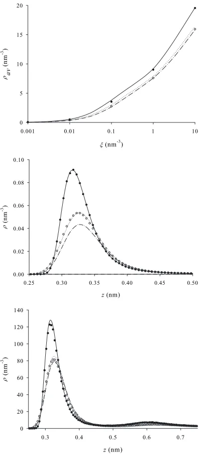
Now that all model parameters have been calibrated we can begin to compare the performance of each technique. First, the 77 K isotherms for the ORA-DFT and FH-DFT techniques are compared with simulation results for the 2.0 nm pore in Fig.7共a兲. Note that the FH-DFT density pro-file is obtained from Eq.共14兲. Also shown in Fig.7共a兲are the corresponding classical results. Results are presented in terms of the average pore density

␳av=

1 H

冕

H

dz␳共z兲 共29兲

as a function of the bulk density. Figure 6 can be used to convert bulk density to the activity␰. We see that the classi-cal simulation and DFT results agree well at low bulk den-sity, which is to be expected because at low density the ex-cess functional, which is known to not be very accurate, plays an insignificant role. As the bulk density increases the excess functional becomes more significant and so the agree-ment deteriorates, even though the Lennard-Jones parameters input to this classical DFT have been calibrated to reproduce the bulk MC simulation isotherm. “Switching on” quantum fluctuations generates the PI-GCMC simulation, ORA-DFT and FH-DFT results. We see good agreement at low bulk density between the PI-GCMC and FH-DFT results, but the FH-DFT results deteriorate at higher bulk densities. Note that the FH-DFT isotherm, relative to the PI-GCMC therm, exhibits similar behaviour to the classical DFT iso-therm, relative to the GCMC results, as bulk density in-creases. This indicates that it is the excess functional, both in the classical DFT and FH-DFT cases, that is generating this error. Conversely, the ORA-DFT result is relatively poor at low bulk density, where the excess functional is insignificant. This happens because the ORA generates too much smooth-ing of the density profile. However, at higher bulk densities agreement between PI-GCMC and the ORA-DFT improves. FIG. 6. Bulk isotherms for models of molecular hydrogen at

77 K. The solid circles are classical GCMC results using the bare hydrogen molecule–hydrogen molecule potential and the solid line corresponds to the best fit to them using the DFT共17兲with param-eters in TableII. The open circles are PI-GCMC results, and the dotted line corresponds to the best fit to them using the ORA-DFT with parameters in TableII. The open triangles are GCMC results using the FH-LJ potential shown in Fig.5, and the dashed-dotted line corresponds to the best fit to them using the FH-DFT with parameters in TableII.

TABLE II. Effective Lennard-Jones parameters used in this study. The FH-LJ parameters are found by fitting a Lennard-Jones potential to the true FH potential obtained via Eq.共10兲. The other parameters are obtained by fitting a bulk isotherm generated by the respective DFT to a bulk isotherm generated by MC simulation

共PI-GCMC for the ORA-DFT method兲.

␦ FH-LJ FH-DFT ORA-DFT DFT

␴eff_{共nm兲 0.3076 0.2908 0.2903 0.2810}

␧eff_/k

This is because of a fortuitous cancellation of errors; the simple DFT used here cancels some of the error inherent in the ORA.

Figures7共b兲 and 7共c兲 provide more insight into this be-haviour. Figure7共b兲 shows a portion of the density profiles corresponding to␰= 0.0001 nm−3, while Fig.7共c兲shows the

density profiles corresponding to␰= 1.0 nm−3_{. The effect of}

including quantum fluctuations is clear; the height of the peak signifying the first adsorbed layer is significantly re-duced, to nearly half its classical value. At␰= 0.0001 nm−3

we see excellent agreement between classical MC simulation and DFT, which must agree perfectly in the low density limit. We also see rather good agreement between the PI-GCMC and FH-DFT results. In contrast, the ORA-DFT den-sity profile is quite poor due to excessive smoothing. How-ever, at␰= 1.0 both the FH-DFT and ORA-DFT results are in reasonable agreement with PI-GCMC results. This change in the accuracy of each method is a reflection of the accuracy of the DFT used forFex.

Similar behavior is observed for the 0.7 nm pore. Figure 8共a兲shows the corresponding average pore density isotherm, while Figs.8共b兲and8共c兲display portions of the density pro-files corresponding to␰= 0.000 001 and␰= 1.0. Note that for both the 2.0 nm and 0.7 nm pores the average pore density is reduced relative to the classical result by over 20% at mod-erate densities, while the peak height in the density profile is reduced by about 40% for the 2.0 nm pore.

If we compare results of Guet al.published in Ref. 关11兴 with those here we see that both the PI-DFT and PI-GCMC results in Ref. 关11兴 are qualitatively incorrect for low bulk densities. In particular, in Figs. 2a, 3a, and 4a in Ref.关11兴we see the effect of including quantum dispersion at 100 and 70 K, relative to the classical result, is very significant. The density peak corresponding to the first adsorbed layer ap-pears to be dramatically reduced, although admittedly the entire classical profile is not reproduced in these figures. This behaviour is qualitatively different to that observed here where the effect of quantum dispersion is much more modest at 77 K. Although these results in Ref. 关11兴 correspond to cylindrical pores, which model carbon nanotubes, and bulk densities in the range 3 to 5 nm−3, these cylindrical pores are sufficiently wide that qualitative comparison with the 2.0 nm slit pore results at␰= 1.0 here关Fig.7共c兲兴is valid. Although we can expect the PI-DFT results in Ref. 关11兴 to be poor 共because of the SAFT-base ring-polymer model used兲, this does not explain why their PI-GCMC results agree with them.

IV. DISCUSSION

The aim of this work is to survey techniques based on classical density functionals able to model hydrogen phys-isorption at low temperature. Only methods able to treat quantum dispersion have been considered. In particular, tech-niques based on the ORA and FH approximations are com-pared at 77 K. To allow consideration of isotherms a density functional treatment of excess共hydrogen molecule–hydrogen molecule兲interactions is developed for both techniques. We find that the FH technique is inherently more accurate than the ORA technique for this problem at low densities. This indicates that the fixed Gaussian wave packet representation of the quantum dispersion of molecular hydrogen at 77 K is accurate for adsorption in graphitic pores. However, the ORA technique is able to cancel some of the error inherent in the excess density functional at moderate and higher densi-FIG. 7.共a兲Average pore density isotherms for hydrogen at 77 K

in a 2.0 nm graphitic pore predicted by each technique: Classical GCMC 共solid circles兲, PI-GCMC 共open circles兲, classical DFT

共solid line兲, FH-DFT共dotted line兲, and ORA-DFT共dot-dashed line兲. Statistical errors are smaller than symbol sizes. The activity␰is on a logarithmic scale. 共b兲 Density profiles for hydrogen at ␰ = 0.0001 nm−3_{and 77 K in a 2.0 nm graphitic slit pore predicted by}

ties. This conclusion does not appear to depend on the slit pore width. So, the ORA-DFT technique is preferred overall unless more accurate density functionals are used to treat excess interactions. Existing density functionals关33,34兴for Lennard-Jones fluids could be used in this context, but it is not yet clear whether they remain accurate in the narrowest pores. Unfortunately, the ORA-DFT technique is somewhat less efficient than the FH-DFT technique because of the ad-ditional numerical demand required to integrate the propaga-tors, and this additional overhead increases linearly withn. Roughly, if the numerical effort required for the FH-DFT technique is proportional to 6 + 2r_c/d, then the effort required for the ORA-DFT technique is 6 + 2rc/d+共n− 1兲/2, if each

propagator integration is carried out on a mesh with the same

number of points as 共but a finer resolution than兲 the hard-sphere fundamental measure functional integrations. At much higher temperatures the ORA-DFT technique should become almost as efficient as the FH-DFT technique because it converges for smaller values ofnat higher temperatures.

Each of these techniques could be applied to model hy-drogen adsorption in real materials such as active carbons and carbon nanotubes, which are often 关31,32兴 modeled in terms of slit or cylindrical pores. Because of the efficiency of each DFT technique, for which solutions are generally ob-tained in a matter of seconds on a desktop PC in this appli-cation to slit pores, they would be particularly suited to op-timization studies of adsorption materials. In this case, the Lennard-Jones parameters could be calibrated by comparison with experimental data for bulk and adsorbed hydrogen rather than by comparison with PI-GCMC simulations. Note that the corresponding PI-MC simulations required tens of minutes to several hours, depending on the value of n, to obtain a satisfactory level of statistical error, which supports the view expressed in the introduction that DFT techniques can find useful applications.

It is interesting to try and understand why the ORA is remarkably accurate for the 3D-QHO problem as well as other central potentials. The problem with the ORA is that the statistics of a chain polymer are not the same as those of the corresponding ring polymer. This is because the end sites 共with labels 1 andn兲are not harmonically bonded as they are in a ring polymer. However, note that for a bulk fluid this final bond has no effect on the bulk density corresponding to a given chemical potential. Moreover, for problems involv-ing attractive central potentials, like the 3D-QHO here and the hydrogen atom problem in Ref. 关4兴, the average site 1–siten separation will reduce relative to its bulk value be-cause of the constraining effect of the external potential. In-deed, this average separation will reduce as the confining external potential becomes stronger, so long as it is a central potential. Essentially, a confining central potential will, on average, “squeeze” these end sites together. This effect will not occur for other kinds of external potential. So, for attrac-tive central potentials we can expect the statistics of chain polymers to converge to those of the corresponding ring polymers as the external potential becomes stronger. By in-terpolation then, because the ORA provides accurate density profiles for a uniform potential and for strongly attractive central potentials, we might also expect it to be accurate for any attractive central potential. For general potentials this is not the case; the ORA generates too much smoothing. More-over, when the number of quantum particles is fixed, as with the application to the 3D-QHO and other central potential problems in Ref. 关4兴, the Lagrange multiplier is chosen to ensure this constraint is satisfied. Essentially, the density pro-file is rescaled to satisfy this condition. This compensates to some degree for any inaccuracy in the ORA. This rescaling is not performed in grand canonical applications such as the hydrogen adsorption problem here, and so for this problem the error inherent in the ORA is more obvious.

Regarding other PI-DFT techniques based on classical density functionals, the method of Guet al.关11兴is shown to be qualitatively incorrect, while the weighted density ap-proximation for bonding 关13兴 can be extended to PI ring FIG. 8.共a兲As for Fig.7共a兲except that the pore is 0.7 nm wide.

共b兲 As for Fig. 7共b兲 except that the pore is 0.7 nm wide, ␰ = 0.000 001 nm−3 _{and only the portion 0.25 nm⬍z⬍0.35 nm is}

polymers but requires calibration in advance, which is incon-venient.

Note that because quantum exchange is significant for electrons in atoms, molecules and solids the methods pre-sented here cannot be applied immediately to model these particles. The most important missing ingredient is the ex-change contribution toFex for electrons, i.e., the exchange functional. In principle, the same exchange-correlation func-tionals used with other electronic structure density functional techniques could be applied to the ORA-DFT method pre-sented here. However, because of the limitations of the ORA we should only expect accurate results for central potential problems, e.g., the electronic structure of atoms and ions.

APPENDIX A: EXACT 3D QHO SOLUTIONS

For a single particle, exact solutions for the particle den-sity are obtained by summing over the appropriately Boltz-mann weighted distribution of quantum state densities. The 3D QHO can be treated as three independent orthogonal lin-ear harmonic oscillators, so the particle density is

␳共r兲= 1 Qn

兺

⬁

␺n_x共x兲␺_n

x

*_{共x兲exp关−␤ប␻共n}

x+ 0.5兲兴

⫻ 1 Q_n

兺

y=0 ⬁

␺n_y共y兲␺n*_y共y兲exp关−␤ប␻共ny+ 0.5兲兴

⫻ 1 Q_n

兺

z=0 ⬁

␺n_z共z兲␺_n

z

*_{共z兲exp关−␤ប␻共n}

z+ 0.5兲兴,

共A1兲

where the partition function,Q, of a linear harmonic oscilla-tor is

Q=

兺

n=0

⬁

exp关−␤ប␻共n+ 0.5兲兴=关2 sinh共␤ប␻/2兲兴−1_,

共A2兲

␺n_x共x兲is the wave function corresponding to energy levelnx

for a 1D QHO corresponding to the x component, and ␻

=

冑

Because the 3D QHO is spherically symmetric we expect the particle density to be conveniently expressed as ␳共r兲, which is equivalent to

␳共x兲= 1 Qn

兺

⬁

␺n_x共x兲␺_n

x

*_{共x兲exp关−␤ប␻共n}

x+ 0.5兲兴

⫻ 1 Q_n

兺

y=0 ⬁

␺_n

y共0兲␺n*_y共0兲exp关−␤ប␻共ny+ 0.5兲兴

⫻ 1 Q_n

兺

z=0 ⬁

␺n_z共0兲␺_n

z

*_{共0兲exp关−␤ប␻共n}

z+ 0.5兲兴.

共A3兲

The wave functions of the 1D QHO are

␺_n共x,t兲=C_nH_n共␥x兲exp关−共␥x兲2/2兴exp共−iE_nt/_ប兲, 共A4兲

where the energy corresponding to each wave function is

En=ប␻共n+ 0.5兲. 共A5兲

In Eq.共A4兲i=

冑

冑

冑

2nn!, and a re-currence relation is used for the Hermite polynomials:

H0= 1,

H₁= 2␣x,

Hn+1共␣x兲= 2␣xHn共␣x兲− 2nHn−1共␣x兲. 共A6兲

Note that although the particle density 共␺n共x兲␺_n*共x兲兲

corre-sponding to individual linear harmonic oscillator states is not spherically symmetric, once the Boltzmann sum over states is performed the particle density is spherically symmetric, as required.

APPENDIX B: STATISTICAL MECHANICS OF PI RING POLYMERS

This appendix deals with the statistical mechanics of non-interacting PI ring-polymers in the canonical ensemble. We need only consider a single ring polymer. From Eq.共1兲 the partition function of one PI ring polymer is

Q1=

冉

n␤␭

␲

冊

3n/2

冕

共B1兲

From this we obtain the density profile of the entire ring polymer

␳共R兲=具␦共R

_⬘

冉

n␤␭

␲

冊

3n/2

冕

_⬘

⫻exp兵−␤关Hintra共R

_⬘

_⬘

_⬘

=Q_c−1exp兵−␤关Hintra共R兲+Hext共R兲兴其, 共B2兲

whereQcis the configurational part of the partition function

Q1. This proves that Eq.共5兲is the correct expression for the

canonical Helmholtz free energy functional because the minimum of Eq. 共5兲 with respect to ␳共R兲 gives Eq. 共B2兲 when multiplied by exp共␤␮兲, where␮is a suitable Lagrange multiplier.

␳i共r兲=具␦共ri−r兲典=

1 Q1

冉

n␤␭

␲

冊

3n/2

冕

whereR=共r1, . . . ,rn兲, which can be written

␳i共r兲=Qc −1

e−␤V共r兲

冕

2

冕

dri−2e−␤V共ri−2兲e−␤n␭ri−1.i−2 2

. . .

冕

⫻

冕

冕

i+2e−␤V共ri+2兲e−␤n␭ri+1.i+2 2

. . .

冕

2

⫻e−␤n␭r1.n

2

. 共B4兲

The open-ring approximation共ORA兲deletes the last bond giving for the middle site

␳_共n+1兲/2共r兲=Qc

−1_e−␤V共r兲_关G

共n−1兲/2共r兲兴2, 共B5兲

whereGis given by Eq.共8兲.

Moreover, we can use a variant of the Percus trick appropriate for intamolecular distributions together with Eq.共B4兲to obtain the bulk total intramolecular distribution function,h_iring_,n 共r兲. So, by settinge−␤V共r1兲₌␦共_r

1兲 共which fixes site 1 at the origin兲

andV共rj⫽1兲= 0, which is appropriate for a uniform system, we first obtain the bulk intramolecular distribution function for

sitei,

h_iring_,n 共r兲=␳i共r兲⬀

冕

2

冕

dri−2e−␤n␭ri−1.i−2 2

. . .

冕

⫻

冕

冕

i+2e−␤n␭ri+1.i+2 2

. . .

冕

2

e−␤n␭兩rn兩2_. 共B6兲

Because of the convolution property of Gaussian functions, this can be written as

h_iring_,n 共r兲=

冉

␤␭

冊

3/2

hlin_i−1共r兲hlin_n−i+1共r兲, 共B7兲

where

hlin_j 共r兲=

冉

冊

3/2

exp共−n␤␭r2_{/j兲. 共B8兲}

Forn odd the total function is then just

h_nring共r兲= 2

兺

i=1 共n−1兲/2

h_iring_,n共r兲. 共B9兲

This converges to the known关38兴limiting result asn→⬁ h_nring共r兲

n− 1 ——→

n=⬁ 2␤␭

␲

exp共− 4␤␭r2_兲

r . 共B10兲

For a chain polymer withnodd the total intramolecular dis-tribution function relative to the middle site is simply

h_nchain共r兲= 2

兺

i=1 共n−1兲/2

h_ilin共r兲. 共B11兲

关1兴R. P. Feynman and A. R. Hibbs,Quantum Mechanics and Path Integrals共McGraw-Hill, New York, 1965兲.

关2兴H. Lowen, J. Phys.: Condens. Matter 14, 11897共2002兲.

关3兴D. Chandler and P. G. Wolynes, J. Chem. Phys. 74, 4078

共1981兲.

关4兴A. Broukhno, P. N. Vorontsov-Velyaminov, and H. Bohr, Phys. Rev. E 72, 046703共2005兲.

关5兴C. E. Woodward, J. Chem. Phys. 94, 3183共1991兲.

关6兴B. H. Zimm and W. H. Stockmayer, J. Chem. Phys. 17, 1301

共1949兲.

关7兴M. Bishop and C. J. Saltiel, J. Chem. Phys. 89, 1159共1988兲.

关8兴H. Tanakaet al., J. Am. Chem. Soc. 127, 7511共2005兲.

关9兴P. Kowalczyket al., Langmuir 23, 3666共2007兲.

关10兴A. Konstantakouet al., Appl. Surf. Sci. 253, 5715共2007兲.

关11兴C. Gu, G. H. Gao, and Y. X. Yu, J. Chem. Phys. 119, 488

共2003兲.

关12兴R. P. Sear and G. Jackson, Mol. Phys. 81, 801共1994兲.

关13兴M. B. Sweatman, J. Phys.: Condens. Matter 15, 3875共2003兲.

关14兴M. B. Sweatman共unpublished兲.

关15兴S. Satyapalet al., Catal. Today 120, 246共2007兲.

关16兴M. Hirscher and B. Panella, Ann. Chim. 共Paris兲 30, 519

共2005兲.

关17兴S. K. Bhatia and A. L. Myers, Langmuir 22, 1688共2006兲.

关19兴J. Turnbull and M. Boninsegni, Phys. Rev. B 76, 104524

共2007兲.

关20兴G. Stan and M. W. Cole, J. Low Temp. Phys. 110, 539共1998兲.

关21兴P. Kowalczyk and J. M. D. MacElroy, J. Phys. Chem. B 110, 14971共2006兲.

关22兴D. Chandler, J. D. McCoy, and S. J. Singer, J. Chem. Phys.

85, 5971共1986兲.

关23兴D. Chandler, J. D. McCoy, and S. J. Singer, J. Chem. Phys.

85, 5977共1986兲.

关24兴R. P. Feynman, Statistical Mechanics 共McGraw-Hill, New York, 1972兲.

关25兴G. A. Voth, Phys. Rev. A 44, 5302共1991兲.

关26兴R. Evans, inFundamentals of Inhomogeneous Fluids, edited by D. Henderson共Wiley, New York, 1992兲.

关27兴Y. Rosenfeld, Phys. Rev. Lett. 63, 980共1989兲.

关28兴E. Kierlik and M. L. Rosinberg, Phys. Rev. A 42, 3382共1990兲.

关29兴S. Phanet al., Phys. Rev. E 48, 618共1993兲.

关30兴J. D. Weeks, D. Chandler, and H. C. Andersen, J. Chem. Phys.

54, 5237共1971兲; 54, 5422共1971兲.

关31兴M. B. Sweatman, inThe Handbook of Theoretical and Com-putational Nanotechnology, edited by M. Rieth and W. Schom-mers 共American Scientific Publishers, Los Angeles, 2006兲, Vol. 5.

关32兴M. B. Sweatman and N. Quirke, Mol. Simul. 31, 667共2005兲.

关33兴M. B. Sweatman, Phys. Rev. E 63, 031102共2001兲.

关34兴M. B. Sweatman, Phys. Rev. E 65, 011102共2002兲.

关35兴J. Wang, J. K. Johnson, and J. Q. Broughton, J. Chem. Phys.

107, 5108共1997兲.

关36兴H. Goldstein, Classical Mechanics 共Addison-Wesley, Red-wood City, CA, 1980兲.

关37兴J. P. Hansen and I. McDonald,Theory of Simple Liquids共 Aca-demic Press, New York, 1990兲.

关38兴J. D. McCoy, S. W. Rick, and A. D. J. Haymet, J. Chem. Phys.