MULTIPLE SHIFT SECOND ORDER SEQUENTIAL BEST ROTATION ALGORITHM FOR
POLYNOMIAL MATRIX EVD
Zeliang Wang
∗, John G. McWhirter
∗, Jamie Corr
†, Stephan Weiss
†∗
School of Engineering
Cardiff University
Cardiff, Wales, UK
†
Department of Electronic & Electrical Engineering
University of Strathclyde
Glasgow, Scotland, UK
ABSTRACT
In this paper, we present an improved version of the second order sequential best rotation algorithm (SBR2) for polyno-mial matrix eigenvalue decomposition of para-Hermitian ma-trices. The improved algorithm is entitled multiple shift SBR2 (MS-SBR2) which is developed based on the original SBR2 algorithm. It can achieve faster convergence than the original SBR2 algorithm by means of transferring more off-diagonal energy onto the diagonal at each iteration. Its convergence is proved and also demonstrated by means of a numerical ex-ample. Furthermore, simulation results are included to pare its convergence characteristics and computational com-plexity with the original SBR2, sequential matrix diagonization (SMD) and multiple shift maximum element SMD al-gorithms.
Index Terms— Polynomial matrix eigenvalue decompo-sition, multiple shift SBR2.
1. INTRODUCTION
The conventional EVD algorithm is suitable for diagonaliz-ing the covariance matrix of narrowband signals. When the problem is extended to broadband scenarios, polynomial ma-trix eigenvalue decomposition (PEVD) techniques need to be taken into account. The idea of the PEVD is generalized as [1]
H(z)R(z)H(z)≈D(z), (1)
whereH(z)is a paraunitary matrix such thatH(z)H(z) =
H(z)H(z) =I, andR(z)is the input para-Hermitian matrix. D(z) is (ideally) a diagonal polynomial matrix. Through-out this paper, polynomial matrices are denoted as under-scored boldface capital letters, and the notation of upon a polynomial matrix denotes the paraconjugate operation. In the case of broadband sensor arrays, the paraunitary matrix
The authors would like to thank the Engineering and Physical Sciences Research Council (EPSRC) Grant number EP/K014307/1 and the MOD Uni-versity Defence Research Collaboration in Signal Processing for partially supporting this work.
H(z)acts as a multichannel all-pass filter, and it aims to di-agonalize the para-Hermitian matrixR(z)by means of pa-raunitary similarity transformation while still preserving the total signal energy [2]. Assuming the received signalsx(t)
have zero mean, the space-time covariance matrix is given by R(τ) = Ex(t)xH(t−τ), where E{·} denotes the expectation, the superscript H denotes Hermitian transpose, andτ ∈ Z. Then the cross-spectral density (CSD) matrix can be defined in terms of thez-transform given byR(z) =
τR(τ)z−τ. Note that the CSD matrix is para-symmetric,
since it satisfies R(z) = R(z). HereR(z)is the paracon-jugate ofR(z), defined asR(z) = RH(1/z), i.e. perform-ing Hermitian transpose of the polynomial coefficient matrix R(τ)and time-reversing all entries inside.
PEVD techniques have attracted lots of interest in digi-tal signal processing and communications over the past few years. Applications of PEVD have been found in areas, such as strong decorrelation of the signals received by broadband sensor arrays [1], broadband angle of arrival estimation [3, 4], subband coding [5], precoding and equalization for multiple-input multiple-output (MIMO) communications [6], spectral factorization [7], and blind source separation [11–13] etc.
Besides the original SBR2 algorithm [1], a number of SMD versions have emerged, including the original SMD al-gorithm [8] and its improved versions, multiple shift max-imum element SMD (MSME-SMD) [9] and the causality-constrained multiple shift SMD [10] algorithm. The SMD family can achieve better diagonalization than SBR2 at the expense of a higher computational cost. Therefore, the aim of this paper is to see whether some of the ideas of MSME-SMD can be harnessed to create a faster converging version of SBR2 that however still enjoys the SBR2 family’s low com-plexity.
2. EXISTING PEVD ALGORITHMS
2.1. Second Order Sequential Best Rotation Algorithm
For each iteration, the SBR2 algorithm [1] starts by locating the maximum off-diagonal element. An elementary delay ma-trix and Jacobi rotation are applied to bring the element onto the zero-lag coefficient matrixR(i−1)(0)∈CM×M, and then rotate its energy onto the diagonal. Here the superscripti de-notes the iteration index. To find the maximum off-diagonal element, we define a matrixS(i)(τ), which contains only the upper triangular elements in R(i−1)(τ) with the remaining elements set to zero. Thus the location of the maximum off-diagonal elements(jki)(τ),(j < k)found ati-th iteration sat-isfies
{j(i), k(i), τ(i)}= arg max
j,k,τS
(i)(τ)∞, (2)
wherej(i),k(i) andτ(i) are the corresponding row, column and time lag index. AssumingP(i)(z)andQ(i)denote the elementary delay and rotation matrix respectively, the maxi-mum off-diagonal elementr(jki)(τ)and its complex conjugate
rkj(i)(−τ)can be transferred onto the diagonal of the zero-lag
(τ = 0)matrixR(i)(0)by performing the following transfor-mations.
R(i)(z) =P(i)(z)R(i−1)(z)P(i)(z), (3)
R(i)(z) =Q(i)R(i)(z)QH(i), (4) whereR(i)(z)stands for the intermediate variable for the el-ementary delay operation. LetE(i)(z)be the elementary pa-raunitary matrix at thei-th iteration, then it can be expressed as
E(i)(z) =Q(i)P(i)(z). (5) The algorithm continues its iterative process until all the off-diagonal elements are smaller than a given thresholdwhich can be set to a very small value to achieve sufficient accuracy. Assuming that the algorithm has converged at theN-th itera-tion, the diagonalized para-Hermitian matrix in (1) takes the form of
D(z) =diag{d1(z), d2(z),· · · , dM(z)}, (6)
and the generated paraunitary polynomial matrix is given by
H(z) =N i=1
E(i)(z) =E(N)(z)· · ·E(2)(z)E(1)(z). (7)
2.2. Sequential Matrix Diagonalization Algorithm
Unlike the SBR2 algorithm, the SMD algorithm [8] requires a initialization step to diagonalize the zero-lag coefficient ma-trix R(0)(0) before all iterations. This is implemented by computing a full EVD toR(0)(0)and then applying the cor-responding modal matrix to the rest of coefficient matrices
R(0)(τ), τ = 0. For thei-th iteration, it starts by locating the column that contains the maximum off-diagonal energy, and then according to the location informationk(i)andτ(i), it shifts the corresponding row and column pair onto the zero-lag plane. As to the rotation step, rather than just using a single Jacobi rotation as with SBR2, the SMD algorithm com-putes a full EVD operation for the zero-lag matrixR(i)(0).
2.3. Multiple Shift Maximum Element SMD Algorithm
The MSME-SMD algorithm [9] introduced a distinguishing search and shift strategy, which can shift more energy than both the SBR2 and SMD onto the diagonal at each iteration. For each iteration, more than one maximum off-diagonal ele-ment is found by using a reduced search space strategy. Ev-ery row and column pair containing a maximum off-diagonal element will then be shifted to the zero-lag matrix. This is different to the way the SMD algorithm operates. The SMD algorithm always shifts the row and column pair containing the maximum off-diagonal energy rather than the maximum off-diagonal element as in MSME-SMD. At the rotation step, the MSME-SMD algorithm follows the same procedure as the SMD algorithm transferring all the off-diagonal elements in R(i)(0)onto the diagonal.
3. MULTIPLE SHIFT SBR2 ALGORITHM
3.1. Outline of Algorithm
The multiple shift SBR2 algorithm (MS-SBR2) was devel-oped based on the SBR2 algorithm, with an additional energy transferred onto the diagonal in every iteration step akin to the MSME-SMD algorithm, so that it can achieve the diago-nalization with less iterations. With MS-SBR2, there are two main steps involved at each iteration. The first step involves multiple shifts operations, and the second step is to perform a sequence of Jacobi rotations corresponding to the multiple shifts. Therefore for thei-th iteration, the elementary parau-nitary matrix in MS-SBR2 can be defined as
E(i)(z) =Q(i)P(i)(z) =
L(i)
l=1 Q(l,i)L
(i)
l=1
P(l,i)(z), (8)
whereQ(i) = lL=1(i)Q(l,i),P(i)(z) = lL=1(i)P(l,i)(z)and
L(i)denotes the total number of off-diagonal elements shifted to the zero-lag coefficient matrix at thei-th iteration. The resulting para-Hermitian matrix at this iteration can be com-puted by performing the similarity transform as
R(i)(z) =P(i)(z)R(i−1)(z)P(i)(z), (9)
R(i)(z) =Q(i)R(i)(z)QH(i)
. (10)
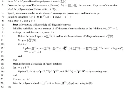
1: InputM×M para-Hermitian polynomial matrixR(z).
2: Compute the square of Frobenius norm (F-norm):N4=R(z)2F, i.e. the sum of squares of the entries of all the polynomial coefficient matricesR(τ).
3: Specify maximum number of iterations,I, convergence parameter,, and trim factorμ. 4: Initialize variables:iter←0,H(0)(z)←Iandg←1 +.
5: whileiter < Iandg >
6: Step 1:locate and shift multiple off-diagonal elements
7: Initialize variables: the total number of off-diagonal elements shifted at thei-th iteration,L(i)←0. 8: whileg > and the search space exists
9: Define the search space inR(i)(z), and locate the maximum off-diagonal element,r(jki)(t). 10: Setg=|r(jki)(t)|
11: ifg >
12: UpdateR(i)(z) =P(i)(z)R(i−1)(z)P(i)(z),H(i)(z) =P(i)(z)H(i−1)(z)according to (3).
13: L(i)←L(i)+ 1
14: end
15: end
16: Step 2:perform a sequence of Jacobi rotations
17: forl= 1 :L(i)
18: UpdateR(i)(z) =Q(i)R(i)(z)QH(i), andH(i)(z) =Q(i)H(i)(z)according to (4).
19: end
20: iter←iter+ 1
21: Trim the polynomial order:R(i)(z)←trim(R(i)(z), μ), according to [1].
[image:3.612.95.520.24.330.2]22: end
Table 1.Summary of the MS-SBR2 Algorithm
The search strategy for MS-SBR2 differs from the one employed in SBR2, and it is based on a set of reduced search spaces. Since each Jacobi rotation operation will act on both the columns and rowsjandkof the maximum off-diagonal elementrjk(i)(0) at the zero-lag plane, the search space for the next off-diagonal element will have to exclude those two columns and rows to avoid the previous off-diagonal element being affected.
Assuming the input para-Hermitian matrix has dimension
6×6, the first off-diagonal element at thei-th iteration can be located according to (2). Once the first elementaand its complex conjugatea∗have been shifted to the zero-lag matrix as shown in Fig. 1(a), the gray areas shown in Fig. 1(b) will be eliminated from the search space of the next off-diagonal element, which leads the white parts of the upper triangular area to be the search space of the second element. By con-tinuing from Fig. 1(b), if the second elementbwas found at row3and column6, its complex conjugateb∗will be at row6 and column3according to the para-Hermitian property. Af-ter bringing them to the zero-lag matrix as shown in Fig. 1(c), the search space for the third elementc∗will be the remaining position row 1 and column 5 shown in Fig. 1(d). This search strategy applies to a generalM ×M para-Hermitian matrix. Generally speaking, there are at mostM/2off-diagonal ele-ments which can be located at each iteration. Therefore, in the case ofM ≤ 3, the MS-SBR2 algorithm is identical to
a
a∗
b
b∗
a
a∗
b
b∗
c∗
c
a
a∗
a
a∗
(a) (b)
(c) (d)
Fig. 1.MS-SBR2 search strategy for a6×6para-Hermitian matrix
showing (a) the first maximum element found, (b) the reduced search spaces, (c) the second maximum chosen, and (d) the last element found.
the SBR2 algorithm. In other words, if there is only one off-diagonal elements shifted to the zero-lag coefficient matrix at each iteration, i.e.L(i)= 1, then MS-SBR2 reduces to SBR2.
[image:3.612.333.545.362.525.2]es-−3 0 3 0
50
−3 0 3 0
50
−3 0 3 0
50
−3 0 3 0
50
−3 0 3 0
50
−3 0 3 0
50
−3 0 3 0
50
−3 0 3 0
50
−3 0 3 0
50
−3 0 3 0
50
−3 0 3 0
50
−3 0 3 0
50
−3 0 3 0
50
−3 0 3 0
50
−3 0 3 0
50
−3 0 3 0
50
−3 0 3 0
50
−3 0 3 0
50
−3 0 3 0
50
−3 0 3 0
50
−3 0 3 0
50
−3 0 3 0
50
−3 0 3 0
50
−3 0 3 0
50
−3 0 3 0 50 lagτ | R ( τ ) |
Fig. 2. Example of5×5 para-Hermitian polynomial matrix in
Sec. 3.2
sential difference is that for MS-SBR2 we have
γ(i)=
L(i)
l=1
|rj(l)k(l)(τ(l))|2 (11)
representing the norm of all the off-diagonal elements found at thei-th iteration.
3.2. Worked Example
In order to demonstrate its capability of diagonalizing a para-Hermitian matrix, a5×5para-Hermitian matrixR(z)with polynomial order of7was taken as the input for testing this algorithm. This random matrix was generated from a matrix A(z) ∈ C5×5 of order 4 with independent, identically dis-tributed zero mean unit variance complex Gaussian entries, withR(z) =A(z)A(z). The input parameters have been set asI= 2000,= 10−3, andμ= 10−4.
The stem plot in Fig. 2 shows the magnitudes of all the elements in R(τ), τ ∈ {−3,−2,· · ·,2,3}, and Fig. 3 de-picts the magnitudes of the elements in the final diagonalized para-Hermitian matrixD(z). In this case, the MS-SBR2 al-gorithm terminated after167th iterations with the converged value of0.001as shown in Fig. 4, bearing in mind that only the first maximum off-diagonal element found at each itera-tion was used to generate the convergence plot, since it is the maximum element found at that iteration.
4. RESULTS
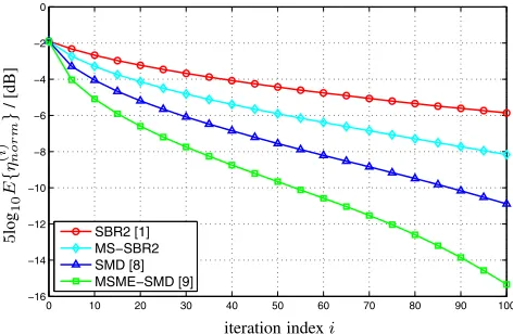
The proposed algorithm was assessed in terms of the normal-ized remaining off-diagonal energy at thei-th iteration. This is defined as
ηnorm(i) =
τ
M
m=1
M
n=1,n=m|rmn(i)(τ)|2
N4{R(z)} , (12)
−3 0 3 0
50 100
−3 0 3 0
50 100
−3 0 3 0
50 100
−3 0 3 0
50 100
−3 0 3 0
50 100
−3 0 3 0
50 100
−3 0 3 0
50 100
−3 0 3 0
50 100
−3 0 3 0
50 100
−3 0 3 0
50 100
−3 0 3 0
50 100
−3 0 3 0
50 100
−3 0 3 0
50 100
−3 0 3 0
50 100
−3 0 3 0
50 100
−3 0 3 0
50 100
−3 0 3 0
50 100
−3 0 3 0
50 100
−3 0 3 0
50 100
−3 0 3 0
50 100
−3 0 3 0
50 100
−3 0 3 0
50 100
−3 0 3 0
50 100
−3 0 3 0
50 100
−3 0 3 0 50 100 lagτ | D ( τ ) |
Fig. 3. Diagonalized polynomial matrix (trimmed) obtained using
the MS-SBR2 algorithm
0 20 40 60 80 100 120 140 160 180
0 2 4 6 8 10 12 14 16 18 20
iteration indexi
| r ( i ) jk ( τ ) |
Fig. 4.Convergence plot of MS-SBR2 for the example in Sec. 3.2
0 10 20 30 40 50 60 70 80 90 100
−16 −14 −12 −10 −8 −6 −4 −2 0 SBR2 [1] MS−SBR2 SMD [8] MSME−SMD [9]
iteration indexi
5 log 10 E { η ( i ) no rm } /[ d B ]
Fig. 5. Comparison of normalized off-diagonal energy among
[image:4.612.56.293.19.207.2] [image:4.612.317.553.21.204.2] [image:4.612.319.554.252.440.2] [image:4.612.317.553.474.628.2]10−1 100 101 −16
−14 −12 −10 −8 −6 −4 −2
SBR2 [1] MS−SBR2 SMD [8] MSME−SMD [9]
mean execution timeE{t}/ [s]
5
log
10
E
{
η
(
i
)
no
rm
}
/[
d
B
]
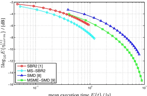
Fig. 6.Normalized off-diagonal energy versus mean execution time
for different PEVD algorithms
where the numerator represents the off-diagonal energy at the
i-th iteration. The comparison among the SBR2, MS-SBR2, SMD and MSME-SMD algorithms is calculated over an en-semble of100realizations of a random6×6para-Hermitian matrixR(z)of order 13, which is generated using the same method mentioned in Sec. 3.2. Fig. 5 shows the normalized remaining off-diagonal energy for various PEVD algorithms within100iterations. Obviously, both the SMD and MSME-SMD algorithms outperform SBR2 and MS-SBR2 in terms of eliminating the off-diagonal energy, and the MS-SBR2 al-gorithm performs better than the SBR2 alal-gorithm since more than one off-diagonal element has been transferred onto the diagonal at each iteration by using the distinguishing search strategy.
[image:5.612.56.294.23.179.2]The mean execution time for each PEVD algorithm has also been measured in order to evaluate the computational cost, and this is implemented in Matlab R2014a on a desk-top PC with characteristics Intel(R) Core(TM) i7-3770T [email protected] GHz and 16 GB RAM. The graph shown in Fig. 6 depicts the remaining off-diagonal energy versus mean execution time. With the same level of diagonalization, the MS-SBR2 algorithm requires the lowest calculation cost compared to the rest of the PEVD algorithms. In contrast, the SMD algorithm requires the longest execution time due to the calculation of the column norms for each search step and the full EVD operation at each iteration.
5. CONCLUSION
We have presented an improved SBR2 algorithm for com-puting the EVD of a para-Hermitian polynomial matrix. Simulation results indicate that the proposed MS-SBR2 al-gorithm provides faster convergence than the conventional SBR2 algorithm, especially in the case of high dimension para-Hermitian matrices. In addition, the MS-SBR2 algo-rithm appears to provide a compromise with much lower computational complexity than the SMD family with respect to computing the decomposition.
REFERENCES
[1] J.G. McWhirter, P.D. Baxter, T. Cooper, S. Redif, and J. Foster, “An EVD Algorithm for Para-Hermitian Poly-nomial Matrices,” IEEE Trans. SP,55(5):2158–2169, May 2007.
[2] P. P. Vaidyanathan,Multirate Systems and Filter Banks, Prentice-Hall, 1993.
[3] M.A. Alrmah, S. Weiss, and S. Lambotharan, “An ex-tension of the MUSIC algorithm to broadband scenarios using polynomial eigenvalue decomposition,” in EU-SIPCO, Barcelona, Spain, pp. 629–633, Sep. 2011. [4] M.A. Alrmah, J. Corr, A. Alzin, K. Thompson, and
S. Weiss, “Polynomial subspace decomposition for broadband angle of arrival estimation,” inSensor Signal Processing for Defence, Edinburgh, Scotland, pp. 1–5, Sep. 2014.
[5] S. Redif, J.G. McWhirter, and S. Weiss, “Design of FIR Paraunitary Filter Banks for Subband Coding Us-ing a Polynomial Eigenvalue Decomposition,” IEEE Trans. SP,59(11):5253–5264, Nov. 2011.
[6] C.H. Ta and S. Weiss, “A Design of Precoding and Equalisation for Broadband MIMO Systems,” in Asilomar Conf. Signals, Systems & Computers, Pacific Grove, CA, pp. 1616–1620, Nov. 2007.
[7] Z. Wang and J.G. McWhirter, “A New Multichan-nel Spectral Factorization Algorithm for Parahermitian Polynomial Matrices,” in10th IMA Int. Conf. Math-ematics in Signal Processing, Birmingham, England, Dec. 2014.
[8] S. Redif, S. Weiss, and J.G. McWhirter, “Sequen-tial Matrix Diagonalization Algorithms for Polynomial EVD of Parahermitian Matrices,” IEEE Trans. SP,
63(1):81–89, Jan. 2015.
[9] J. Corr, K. Thompson, S. Weiss, J.G. McWhirter, S. Redif, and I.K. Proudler, “Multiple shift maximum element sequential matrix diagonalisation for paraher-mitian matrices,” inIEEE SSP, Gold Coast, Australia, pp. 312–315, Jun. 2014.
[10] J. Corr, K. Thompson, S. Weiss, J.G. McWhirter, and I.K. Proudler, “Causality-constrained multiple shift se-quential matrix diagonalisation for parahermitian ma-trices,” inEUSIPCO, Lisbon, Portugal, pp. 1277–1281, Sep. 2014.
[11] P. Comon, and L. Rota, “Blind separation of inde-pendent sources from convolutive mixtures,” IEICE Trans. FECCS,E86-A(3):542–549, Mar. 2003. [12] S. Icart, P. Comon, and L. Rota, “Blind paraunitary
equalization,”Signal Processing,89:283–290, 2009. [13] M. Sorensen, L. De Lathauwer, S. Icart, and L. Deneire,