Structural patterns in complex networks through spectral analysis

Structural Patterns in Complex Networks through

Spectral Analysis

Ernesto Estrada,

Department of Mathematics and Statistics, Department of Physics and Institute of Complex Systems, University of Strathclyde, Glasgow,

G1 1XQ U.K.

Abstract. The study of some structural properties of networks is introduced from a graph spectral perspective. First, subgraph centrality of nodes is defined and used to classify essential proteins in a proteomic map. This index is then used to produce a method that allows the identification of superhomogeneous networks. At the same time this method classify non-homogeneous network into three universal classes of structure. We give examples of these classes from networks in different real-world scenarios. Finally, a communicability function is studied and showed as an alternative for defining communities in complex networks. Using this approach a community is unambiguously defined and an algorithm for its identification is proposed and exemplified in a real-world network.

Keywords: subgraph centrality, Estrada index, communicability, network communities.

1 Introduction

Spectral graph theory is a well established branch of the algebraic study of graphs [9]. Despite there are many results in this field they are mostly applicable to small graphs and not to gigantic complex networks having thousands or even millions of nodes. Without an excess of criticisms it can be said that many of the bound found in spectral graph theory are very far from the real value when applied to large graphs, which make these approximation useless for practical purposes. On the other hand, the study of spectral properties of complex networks has been mainly focused to the study of the spectral density function in certain classes of random graphs [10-13]. This gives little information about the structure of real-world complex networks, which differ from random graphs in many structural characteristics.

Here we attack the problem from a different perspective. We attempt the definition of some spectral invariants for nodes and networks which give important structural information about the organization of these very large graphs. First, we study the characterization of local spectral invariants, in particular subgraph centrality [14] as a way for accounting for a ‘mesoscale’ characterization of nodes in a network. Using this concept we show analytically the existence of four universal topological classes of networks and give examples from the real-world about each of them [15, 16]. Finally, we study a communicability function [17] which allows to identify communities in complex networks [17, 18].

2 Background

We consider here networks represented by simple graphs G:=

(

V,E

)

. That is, graphs having V =n nodes and E =m links, without self-loops or multiple links between nodes. Let A

( )

G =A be the adjacency matrix of the graph whose elements

ij

A are ones or zeroes if the corresponding nodes i and j are adjacent or not, respectively. A walk of length k is a sequence of (not necessarily different) vertices

k k v

v v

v0, 1,, −1, such that for each i=1,2,k there is a link from vi−1 to vi.

Consequently, these walks communicating two nodes in the network can revisit nodes and links several times along the way, which is sometimes called “backtracking walks.” Walks starting and ending at the same node are named closed walks.

Let λ1≥λ2≥≥λn be the eigenvalues of the adjacency matrix in the

non-increasing order and let ϕ_j

( )

p be the pth entry of the jth eigenvector which is associated with the eigenvalue λj [9]. The number of walks µk

( )

p,q of length k

from node p to q is given by

( )

( )

( ) ( )

k

j j n

j j pq

k

k pq ϕ pϕ qλ

µ

∑

=

= =

1

3 Local patterns: Subgraph centrality

A ‘centrality’ measure is a characterization of the ‘importance’ or ‘relevance’ of a node in a complex network. The best known example of node centrality is the “degree centrality”, DC [4], which is interpreted as a measure of immediate influence of a node over its nearest neighbors. Several other centrality measures have been studied for real world networks, in particular for social networks. For instance, betweenness centrality (BC) measures the number of times that a shortest path between nodes i

and j travels through a node k whose centrality is being measured. On the other hand, the farness of a node is the sum of the lengths of the geodesics to every other vertex. The reciprocal of farness is closeness centrality (CC). A centrality measure, which is not restricted to shortest paths [4], is defined as the principal or dominant eigenvector of the adjacency matrix A of a connected network. This centrality measure simulates a mechanism in which each node affects all of its neighbors simultaneously [4]. In fact, if we designate the number of walks of length L starting at node

i

by N_L

( )

i and the total number of walks of this length existing in the network by NL

( )

G . The probability that a walk selected at random in the network has

started at node

i

is simply[19]:

( )

_{( )}

( )

G N

i N i P

L L L = .

(2)

Then, for non-bipartite connected network with nodes 1,2,,n, it is known that for

∞ →

L , the vector

[

PL

( )

1 PL

( )

2  PL

( )

n

]

tends toward the eigenvector centrality

of the network [19]. Consequently, the elements of EC represent the probabilities of selecting at random a walk of length L starting at node i when L→∞:

( )

i P

( )

i EC = L .

If we compare degree and eigenvector centrality we can see that the first account for very local information about the interaction of a node and its nearest neighbors only. However, eigenvector centrality accounts for a more global environment around a node, which in fact includes all nodes of the network. Then, an intermediate characterization of the centrality of a node is needed in such a way that regions closest to the node in question make a larger contribution than those regions which are far apart from it. This sort of ‘mesoscopic’ type of centrality is obtained by considering the subgraph centrality of a node.

The subgraph centrality of a node is defined as the weighted sum of all closed walks starting and ending at the corresponding node [14]. If we designate by µk

( )

i

the number of such closed walks of length k starting and ending at node i, the subgraph centrality is given by

( )

_∑

∞

( )

=

= 0 !

k k

k i i

EE µ , (3)

realize that the subgraph centrality of node i converges to the ith diagonal entry of the exponential of the adjacency matrix:

( ) ( ) ( )

( ) ( )

( )

( )

. ! ! 3 ! 2 ! ! 3 ! 2 3 2 3 2 ii ii k ii k ii ii ii ii e k k i EE A A A A A I A A A A I =         + + + + + + = + + + + + + =     (4)

This index can be expressed in terms of the spectrum of the adjacency matrix of the corresponding network as [14]:

( )

_∑

[ ]

( )

= = n j j j e i i EE 1 2 λ

ϕ , (5)

where ϕj

( )

i is the ith entry of the eigenvector associated with the jth eigenvalue

j

λ of the adjacency matrix.

The subgraph centrality can be split into the contributions coming from odd and even closed walks as follows [20]:

( )

( )

( )

[ ]

( )

( )

[ ]

( )

( )

j

j j j j j even

odd i EE i i i

EE i

EE ϕ sinhλ ϕ 2coshλ

1 2 1

∑

∑

= = + = +

= , (6)

The sum of all subgraph centralities for the nodes of a network is known as the Estrada index of the graph and has been extensively studied in the mathematical literature (see [21, 22] and references therein):

( )

_∑

( )

( )

_∑

= = = = = n j A n i j e e tr i EE G EE 1 1 λ

. (7)

[image:5.595.233.372.145.283.2]

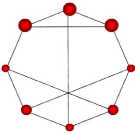
Fig. 1. Illustration of a simple graph in which all nodes have the same degree, closeness and eigenvector centralities. Subgraph centrality differentiates between three types of nodes, which are drawn with sizes proportional to EE

( )

i .

A real-world example of the utility of centrality measures is provided by the identification of essential proteins in a protein-protein interaction (PPI) network. A PPI is a map of the physical interactions taken place between proteins in a cell. These interactions between proteins are responsible for many, if not all, biological functions of proteins in a cell. In every organism there are some proteins which are essential for the functioning of its cells. Knocking out these essential proteins produces the death of this organism. If such organism is a pathogenic one, then essential proteins are good targets for drugs attempting to kill such pathogen. Consequently, the in silico

identification of essential proteins can play an important role in drug design by accelerating the process in which some protein targets are identified. Here an example is provided about the utility of centrality measures in identifying such essential proteins in the yeast PPI.

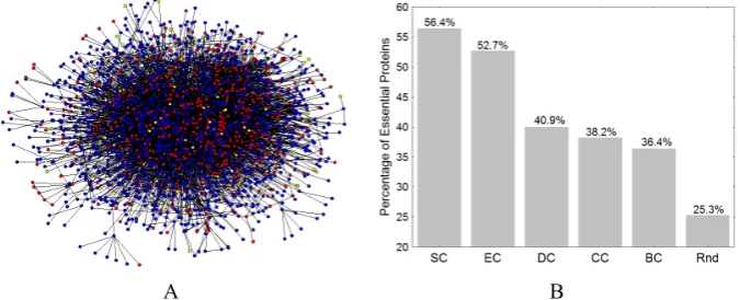
The PPI of Saccharomycescerevisiae (yeast) was compiled by Bu et al. [23] from data obtained by von Mering et al. [24] by assessing a total of 80,000 interactions among 5400 proteins by assigning each interaction a confidence level. Here we study the main connected component of this network consisting of 2224 proteins sharing 6608 interactions. They were selected from 11,855 interactions between 2617 proteins with high and medium confidence in order to reduce the interference of false positives, from which Bu et al. [23] reported a network consisting of 2361 nodes and 6646 links (http://vlado.fmf.uni-lj.si/pub/networks/data/bio/Yeast/Yeast.htm). We illustrate the main connected component of this PPI in Fig. 2A.

significantly larger percentages of essential proteins identified than the random selection method. Both spectral methods used, the eigenvector centrality and the subgraph centrality, identify more than 50% of essential proteins in this proteome. In particular, subgraph centrality identifies 56.4% of essential proteins in the top 5% of the proteins [25]. In closing, centrality measures which are based only on topological information contained in the PPI network account for important biological information of yeast proteome.

A B

Fig. 2. (A) Illustration of the protein-protein interaction (PPI) network of yeast. Every node represents a protein and two nodes are linked if the corresponding proteins have been found to interact physically. Red nodes represent essential proteins, blue represent non-essential and yellow represent proteins with unknown essentiality. (B) Percentage of essential proteins identified by different centrality measures in the yeast PPI. SC, EC, DC, CC and BC stand for subgraph, eigenvector, degree, closeness and betweenness centrality, and Rnd stands for the average of 1000 random realizations.

3 Global patterns

3.1 Structural classes of networks

The simplest class of networks we can consider is one consisting of very homogeneous structure. In these networks ‘what you see locally is what you get globally’. Thus, describing the structure of a part of these networks gives an idea of their global topological structures. In order to have a quantitative criterion for classifying these networks we can consider a subset of nodes S⊆V with cardinality

[image:6.595.129.467.241.378.2]

( )

, 2

0 , , inf

   

   

+∞ < ≤ < ⊆ ∂

= S V S V

S S G

φ (8)

In a ‘superhomogeneous’ network as the ones described in the previous paragraph it is expected that φ

( ) ( )

G =O1

,

which means that the number of links inside the subset

S is approximately the same as the number of links going out from it for all the subsets S⊆V in the network. This means that high expansion implies high homogeneity and better connectivity of the network, which means that the number of links that must be removed to separate the network into isolated chunks is relatively high in comparison with the number of nodes in the network.

A well-known result in spectral graph theory relates the expansion constant and the eigenvalues of the adjacency matrix. That is, if G is a regular graph with eigenvalues

n

λ λ

λ₁≥ ₂≥≥ , then the expansion factor is bounded as [26],

( )

₁

(

_{1 2}

)

2

1 ₂

2 φ λ λ λ

λ

λ − _{≤ ≤ −}

G , (9)

which means that a network has good expansion if the gap between the first and second eigenvalues of the adjacency matrix (∆λ=λ2−λ1) is sufficiently large. In closing, a superhomogeneous network, also known as expander, is characterized by a very large spectral gap ∆λ=λ₂−λ₁.

Let us consider what happen to the subgraph centralilty in these superhomogeneous networks. Without any loss of generality we study here the contribution of odd closed walks to the subgraph centrality EE_odd

( )

i . We can write the expression (5) in the following way by noting that EC

( )

i =ϕ1

( )

i

( )

[

( )

]

sinh

( )

[ ]

( )

2sinh

( )

,

2 1 2

j j j

odd i ECi i

EE λ

∑

ϕ λ

=

+

= , (10)

Because the network we are considering here is a superhomogeneous one we can assume that λ >>1 λ2 in such a way that

( )

[

]

( )

[ ]

( )

( )

j

j j i

i

EC sinhλ γ 2sinhλ 2

1

2

∑

=

>> , (11)

Consequently, in a superhomogeneous network we can approximate the odd-subgraph centrality as,

( )

i

[

EC

( )

i

]

2sinh

( )

λ

1

EEodd ≈ _, (12)

which can be written as a straight line by applying logarithm as [15]:

( )

[

ECi

]

logA log

[

EE_odd

( )

i

]

log = +

η

, ₍₁₃₎

where, A≈

[

sinh

( )

λ1

]

−0.5 and η≈0.5.

environment giving a measure of the cliquishness of a close neighbourhood around it. Consequently, in a superhomogeneous network a log-log plot of EC

( )

i vs. EE_odd

( )

i

displays a perfect straight line fit

( )

0.5log

( )

0.5log

[

sinh

( )

1

]

logECHomoi = EEodd i − λ , (14)

indicating a perfect scaling between local and global environment of a node. In other words, “what you see locally is what you get globally” in such networks. Deviations from perfect superhomogeneity can be accounted by measuring the departure of the points from the straight line respect to _logECHomo

( )

i _[16]:

( )

_log

( )

_{( )}

_log

[

( )

]

2sinh

_{( )}

( )

1 0.5 log         = = ∆ i EE i EC i EC i EC i EC odd Homo λ

, (15)

Then, using (15) a network with ∆logEC

( )

i ≅0is classified as superhomogeneous. Other three classes can be identified, which correspond, respectively to the following cases [16]:

(i) ∆logEC

( )

i ≤0 for all nodes: what you see locally is more densely connected that what you get globally, which indicates that the network contains ‘holes’ in its structure,

(ii) ∆logEC

( )

i ≥0 for all nodes: what you see locally is less densely connected that what you get globally, which indicates the existence of a core-periphery structure of the network,

(iii) ∆logEC

( )

i ≤0 for some nodes and ∆logEC

( )

i >0 for the rest, which indicates the existence of a combination of the previous two patterns in a network.

The negative and positive deviations from the perfect scaling can be accounted by

( )

( )

∑

+ + +         = i i N Ideal 1 1 log 1 γ γ

ξ and

∑

₋

( )

_{( )}

− −         = i i N Ideal 1 1 log 1 γ γ ξ

where

∑

₊ and

∑

₋ are the sums carried out for the N+ points having

( )

0 log ₁ >

∆ γ i and for the N− having ∆logγ1

( )

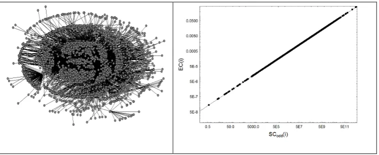
i <0, respectively. In Fig. 3 we illustrate these three patterns of networks together with their spectral scaling.

Network Model

Spectral Scaling

A)

_[

_EClog

_{( )}

_i

_]

2_sinh

( )

_{( )}

0_{1 EE}

_{( )}

_{i, i V.}

i EC

odd ∀ ∈

≤ ⇒ ≤ ∆

B)

_[

_EClog

_{( )}

_i

_]

2_sinh

( )

_{( )}

0_{1 EE}

_{( )}

_{i, i V.}

i EC

odd ∀ ∈

≥ ⇒ ≥ ∆

λ

[image:10.595.122.501.468.623.2]

Fig. 3. Illustration of the three patterns of networks that deviate from perfect spectral scaling. The spectral scaling is a log-log plot of the eigenvector centrality, EC(i) versus subgraph centrality, EE(i) for all nodes in the graph.

In Fig. 4 we illustrate one example of each of the four structural patterns found in complex networks. The first network is a 1997 version of Internet at autonomous system, which displays a large homogeneity as can be seen in the perfect spectral scaling given in the same figure. The negative and positive deviations from perfect scaling for this network are 6.21×10−4 and 1.20×10−3, respectively. The second network corresponds to the residue-residue interaction network in the protein with Protein Data Bank code (1ash), which corresponds to the structure of Ascaris suum

Fig. 4. Illustration of the four structural patterns in real-world complex networks. The first corresponds to Internet autonomous system in 1997, the second is the protein residue network of 1ASH, the third represents a food web of Canton Creek and the fourth corresponds to a social network of friendship ties in a karate club.

A characteristic feature of all networks which are not superhomogeneous is that nodes can be grouped together in certain clusters or communities. These communities can play an important role in understanding the structure and dynamics of complex networks in different scenarios. There are several approaches to detect communities in networks which are used today [28]. In the following section we explain one which is based on the concept of communicability between nodes in a network.

3.2 Communicability and communities in networks

In continuation with the line we have followed in the previous sections we define the communicability between a pair of nodes in a network as follows [17]:

The communicability between a pair of nodes p,q in a network is a weighted sum of all walks starting at node p and ending at node q, giving more weight to the shortest walks.

This definition accounts for the known fact that in many situations the communication between a pair of nodes in a network does not take place only through the shortest path connecting them. A mathematical formulation of this concept is obtained by considering the sum of all walks of different lengths that connect nodes p and q

[17]:

( ) ( )

pq

k

pq k

pq _k e

G ₌

∑

∞ A ₌ A

=0 !

, (16)

which can be expressed in terms of the eigenvalues and eigenvectors of the adjacency matrix as follows

( ) ( )

∑

=

= n

j j j pq p qe j

G

1

λ

ϕ

ϕ

.

(17)

The detection of communities by using the communicability function is based on the analysis of the sign of the term

( ) ( )

_{p qe} j

j j ϕ λ

the principal eigenvector ϕ1 have the same sign. Consequently, we consider it as a translational movement of the whole network. Then, we can divide the communicability function into three contributions [17]:

( ) ( )

[

]

_∑

( ) ( )

_∑

−

( ) ( )

≤ ≤ − ≤ ≤ + +

= inter cluster

2 cluster intra 2 1 1 1 n j j j n

j j j

pq p qe p qe j p q e j

G ϕ ϕ λ ϕ ϕ λ ϕ ϕ λ (18)

where the term ‘intra-cluster’ refers to the sum over all components ϕj

( )

p and ϕj

( )

q

having the same sign. The ‘inter-cluster’ term refer to the case when ϕ_j

( )

p and

( )

q

j

ϕ have different signs. Note that the last term, i.e., the inter-cluster’ communicability is negative. Then, as we are interested in partitioning the network into communities or clusters we simply subtract the translational contribution to obtain the difference between intra- and inter-cluster communicability [17]:

( ) ( )

_∑

( ) ( )

∑

= = − =

∆ inter-cluster

2 cluster -intra 2 j j j j j j

pq p qe j p qe j

G ϕ ϕ λ ϕ ϕ λ

.

(19)

Note that for computing (19) it is not necessary to make any sign analysis of the eigenvectors of the network. It is enough to compute the communicability between two nodes and then subtract the translational term, i.e.,

( ) ( )

1

1

1 ϕ λ

ϕ p qe G

Gpq = pq−

∆ .

Now, we can define a community in a network as follows [18]:

A network community is a group of nodes C⊆V for which the intra-cluster communicability is larger than the inter-cluster one:

C q p Gpq > ∀ ∈

∆ , (β) 0 ( , ) .

In practice, in order to find such communities we represent the values of ∆Gp,q

between pairs of nodes as a matrix ∆(G) and then we dichotomize such matrix, such that the p,q entry of the new matrix is 1 if, and only if ∆Gp,q >0 and zero

otherwise. This new matrix can be considered as the adjacency matrix of a new graph, which we call the communicability graph Θ(G)[18]. The nodes of Θ(G) are the same as the nodes of G, and two nodes p and q in Θ(G) are connected if, and only if, ∆G_p,q >0 in G. Finally, a community is identified as a clique in the communicability graph [18].

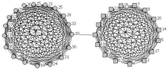
As an example we illustrate in Fig. 5 the communicability graph for the social network of friendship ties in a karate club given in Fig. 4. The analysis of the cliques in this communicability graph indicates the existence of 5 overlapped communities, which are given below:

} 10 , 3 { :

5

[image:14.595.167.435.175.287.2]

C .

Fig. 5. Communicability graph for the network of friendship ties in a karate club. Circles and squares are used to represent the two known communities existing in this network as a consequence of its polarization as followers of the administrator and followers of the trainer.

The overlap between two communities Ci and Cj can be computed by using an

appropriate index SC_iC_j [18]. Then, communities can be merged together according

to a given mergence parameter αin such a way that a new matrix is created according to

   

= <

≥ =

j i C

C C C C

C _{S C C}

S O

j i

j i j

i 0 if , or

if 1

α α

,

and the process is finished when no pair of communities have overlap larger than α. Applying this criterion with α=0.5 the following two communities are obtained for the previously studied network: U₁=C₁∪C₂∪C₃∪C₅ and U₂ =C₄∪C₅, which are the two communities observed experimentally for this network.

4 Conclusions

properties of nonaffine deformation and dissipation, spatially and with respect to strain. On the other hand, communicability was used as a classifier in human brain networks [33]. In this work two groups of brain networks are studied, one group corresponds to healthy humans and the other to patients who suffer stroke in the last six months. The discriminating power of the communicability function of a normalized weighted matrix was higher than other spectral methods for differentiating between the two studied groups. All these examples show the versatility of these spectral measures for studying the structure and properties of complex networks.

Acknowledgments. This work is partially funded by the Principal of the University of Strathclyde through the New Professors’ Fund.

References

1. Strogatz, S.H.: Exploring complex networks. Nature 410, 268--276 (2001)

2. Albert, R., Barabási, A.-L.: Statistical mechanics of complex networks. Rev. Mod. Phys. 74, 47--97 (2002)

3. Newman, M.E.J.: The structure and function of complex networks. SIAM Rev. 45, 167--256 (2003)

4. Newman, M.E.J.: Networks. An Introduction. Oxford University Press, Oxford (2010) 5. Boccaletti, S., Latora, V., Moreno, Y., Chavez, M., Hwang, D.-U.: Complex Networks:

Structure and Dynamics. Phys. Rep. 424 175--308 (2006)

6. Barrat, A., Barthélemy, M., Vespignani, A.: Dynamical Processes on Complex Networks. Cambridge University Press, Cambridge (2008).

7. Watts, D.J., Strogatz, S.H.: Collective dynamics of “small-world” networks. Nature 393, 440--442 (1998)

8. Barabási, A.-L, Albert, R.: Emergence of scaling in complex networks. Science 286, 509--512 (1999)

9. Cvetković, D., Rowlinson, P., Simić, S.: An Introduction to the Theory of Graph Spectra. Cambridge University Press, Cambridge (2010)

10.Farkas, I.J., Derényi, I., Barabási, A.-L., Vicsek, T.: Spectra of “Real–World” Graphs: Beyond the Semi-Circle Law. Phys. Rev. E 64, 026704 (2001)

11.Goh, K.-I., Kahng, B., Kim, D.: Spectra and eigenvectors of scale-free networks. Phys. Rev. E 64, 051903 (2001)

12.Dorogovtsev, S.N., Goltsev, A.V., Mendes, J.F.F.,Samukhin, A.N.: Spectra of complex networks. Phys. Rev. E 68, 046109 (2003)

13.De Aguiar, M.A.M., Bar-Yam, Y.: Spectral analysis and the dynamic response of complex networks. Phys. Rev. E 71, 016106 (2005)

14.Estrada, E., Rodríguez-Velázquez, J.A.: Subgraph centrality in complex networks. Phys. Rev. E 71, 056103 (2005).

15.Estrada, E.: Spectral scaling and good expansion properties in complex networks. Europhys. Lett. 73 649--655 (2006)

16.Estrada, E.: Topological Structural Classes of Complex Networks. Phys. Rev. E 75, 016103 (2007)

18.Estrada, E., Hatano, N.: Communicability Graph and Community Structures in Complex Networks. Appl. Math. Comput. 214, 500--511 (2009)

19.Cvetković, D., Rowlinson, P., Simić, S.: Eigenspaces of Graphs. Cambridge University Press, Cambridge (1997)

20.Estrada, E., Rodríguez-Velázquez, J. A.: Spectral measures of bipartivity in complex networks. Physical Review E 72, 046105 (2005)

21.Deng, H., Radenković, S., Gutman, I.: The Estrada Index. In: Cvetković, D., Gutman, I. (eds.) Applications of Graph Spectra, pp. 123--140. Math. Inst., Belgrade (2009)

22.Benzi, M., Boito, P.: Quadrature rule-based bounds for functions of adjacency matrices. Lin. Alg. Appl. 433, 637--652 (2010).

23.Bu, D., Zhao, Y., Cai, L., Xue, H., Zhu, X., Lu, H., Zhang, J., Sun, S., Ling, L., Zhang, N., Li, G., Chen, R.: Topological structure analysis of the yeast protein-protein interaction network of budding yeast. Nucl. Ac. Res. 31, 2443--2450 (2003)

24.von Mering, C., Krause, R., Snel, B., Cornell, M, Oliver, S. G., Field, S., Bork. P.: Comparative assessment of large-scale data sets of protein-protein interactions. Nature417, 399--403 (2002)

25.Estrada, E.: Virtual identification of essential proteins within the protein interaction network of yeast. Proteomics 6, 35--40 (2006)

26.Hoory, S., Linial, N., Wigderson, A.: Expander graphs and their applications. Bull. Am. Math. Soc. 43 439--561 (2006)

27.Estrada, E.: Universality in Protein Residue Networks, Biophys. J. 98, 890--900 (2010) 28.Fortunato, S.: Community detection in graphs. Phys. Rep. 486, 75--174 (2010)

29.Estrada, E., Higham, D.J., Hatano, N.: Communicability betweenness in complex networks. Physica A 388, 764--774 (2009)

30.Estrada, E., Higham, D.J., Hatano, N.: Communicability and multipartite structure in complex networks at negative absolute temperatures. Phys. Rev. E 78, 026102 (2008) 31.Estrada, E.: Generalized walks-based centrality measures for complex biological networks,

J. Theor. Biol. 263, 556--565 (2010)

32.Walker, D.M., Tordesillas, A.: Topological evolution in dense granular materials: A complex networks perspective. Int. J. Sol. Struct. 47, 624--639(2010)

33.Crofts, J.J., Higham, D.J.: