S
TRATHCLYDE
D
ISCUSSION
P
APERS IN
E
CONOMICS
MODELING U.S. INFLATION DYNAMICS:
A BAYESIAN NONPARAMETRIC APPROACH
B
Y
MARKUS JOCHMANN
N
O
.
10-01
D
EPARTMENT OF
E
CONOMICS
Modeling U�S� Inflation Dynamics:
A Bayesian Nonparametric Approach
Markus Jochmann
Department of Economics, University of Strathclyde [email protected]
January 2010
�bstract
This paper uses an infinite hidden �arkov model �IHMM) to analyze U.S. in-flation dynamics with a particular focus on the persistence of inin-flation. The IHMM is a Bayesian nonparametric approach to modeling structural breaks. It allows for an unknown number of breakpoints and is a flexible and attractive alternative to existing methods. We found a clear structural break during the recent financial crisis. Prior to that, inflation persistence was high and fairly constant.
JEL classifications: C11, C22, E31
1
Introduction
There is ample evidence in the literature that many macroeconomic and financial time series display structural instability (see, e.g., Stock and Watson, 1996, or Ang and Bekaert, 2002). Ignoring this feature in model specification can lead to mislead-ing conclusions and is a main source of poor forecasts. These implications have been shown by, among others, Clements and Hendry (1999) and Koop and Potter (2001). Possible changes in the inflation process and its persistence have received espe-cially much attention in the literature. Inflation persistence, i.e. the speed with which inflation returns to its base level after a shock, is important for many aspects of macroeconomics in general and monetary policy in particular. Probably most importantly, it is at the heart of the revisionism debate initiated by Taylor (1998). He warned that the decline in the persistence of inflation might lead policymakers to return to the belief that there is an exploitable trade-off between inflation and unem-ployment in the long run. Additionally, empirical evidence on inflation persistence informs theoretical researchers as to the importance, or lack thereof, of allowing for a dynamically changing inflation persistence in models of price adjustment. Finally, empirical results also help answer the question whether not only monetary policy has changed in the U.S., but also the response of inflation to monetary shocks.
However, the empirical evidence on the properties of inflation persistence in the literature is ambiguous. On one hand, Cogley and Sargent (2001) use a multivariate time-varying parameter model and find that inflation persistence increased in the early 1970s, remained high for around a decade and declined afterwards. Their result is in accordance with the findings of Brainard and Perry (2000) and Taylor (2000). On the other hand, Stock (2001) applies univariate methods and finds that inflation persistence was roughly constant and high over the past 40 years. This view is also supported by Pivetta and Reis (2007).
The IHMM is a nonparametric Bayesian extension of the hidden Markov model
(HMM). A nonparametric Bayesian model is a probability model with infinitely many parameters (Bernardo and Smith, 1994), or, in other words, a parametrized model that allows the number of parameters to grow with the number of observations. However, for a given sample size it will only select a finite subset of the available parameters to explain the observations. This means that, unlike the HMM, the IHMM does not fix the number of underlying states a priori, but infers them from the data. Thus, the IHMM is an attractive alternative to existing change-point models that typically either assume a small number of change-points (e.g. Chib, 1998) or assume that the parameters change at each point in time. The latter is referred to as the time-varying parameter (TVP) model (e.g. Cogley and Sargent, 2001). Other approaches that allow for a random number of change-points are Koop and Potter (2007), who propose a model where regime durations have a Poisson distribution, or Giordani et al. (2007), who present a state-space model that accounts for parameter instability and outliers, but does not force the parameters to change at each point in time.
The rest of this paper is organized as follows. In Section 2 we first summarize the Dirichlet process and the hierarchical Dirichlet process, which are the building blocks of the IHMM. We then discuss the IHMM and an augmented version of it. Finally, we analyze the choice of hyperparameters and prior distributions and point out how inference can be done using Markov chain Monte Carlo methods. Further details on the sampling algorithm are given in the Appendix. Section 3 uses the IHMM to model U.S. inflation dynamics and Section 4 concludes.
2
The Infinite Hidden Markov Model
The Dirichlet Process
TheDirichlet process (DP) introduced by Ferguson (1973) is a measure on measures defined by the following property: A random probability measure G is generated by a DP if for any partition B1� . . . � Bm on the space of support of G0 the vector
of probabilities [G(B1)� . . . � G(Bm)] follows a Dirichlet distribution with parameter
Sethuraman (1994) showed that any drawG∼DP(α� G0) can be represented as
G=
∞
�
k=1 πkδθ∗
k� (1)
where �θ∗
k}
∞
k=1 represent a set of support points drawn i.i.d. from G0 and δθ∗
k is a
probability measure concentrated at θ∗
k. The probability weights π = �πk}∞k=1 are
coming from a stickbreaking process:
πk =ξk k−1
�
l=1
(1−ξl) with ξl iid
∼ Beta(1� α)� (2)
which we denote by π ∼Stick(α).1 We can see that any draw Gfrom a DP(α� G0)
is discrete and can be represented as an infinite mixture of point masses δθ∗
k.
Another representation of the DP that highlights its discrete nature is the P´olya urn scheme of Blackwell and MacQueen (1973). The P´olya urn scheme does not consider G directly but refers to draws θ1� θ2� . . . from G. Blackwell and MacQueen (1973) show that the conditional distribution ofθigivenθ1� . . . � θi−1has the following
form:
θi|θ1� . . . � θi−1 ∼
i−1
�
j=1
1
i−1 +αδθj + α
i−1 +αG0. (3)
This means that θi takes on the same value as θj with probability proportional to 1
and is drawn from the base measureG0 with probability proportional toα. Clusters emerge since θi has a positive probability of being equal to previous draws. Letting
θ∗
1� . . . � θ
∗
K denote the distinct values taken on byθ1� . . . � θi−1, we can express equation
(3) as
θi|θ1� . . . � θi−1∼
K
�
k=1 mk
i−1 +αδθk∗+ α
i−1 +αG0� (4)
where mk is the number of θi taking the value θ
∗
k.
If we further introduce indicator variabless1� s2� . . .withsi=kindicatingθi =θ
∗
k
�
Another notation for the stick-breaking process is π ∼ GEM��), where the letters refer to
we obtain
Pr(si=s|s1� . . . � si−1) =
K
�
k=1 mk
i−1 +αδ(s� k) + α
i−1 +αδ(s� K+ 1)� (5)
where δ(s� k) denotes the Kronecker delta2. Equation (5) induces a distribution on
partitions and is referred to as the Chinese restaurant process (CRP, see Pitman, 2006) which is a helpful metaphor for understanding the properties of the DP. Con-sider a Chinese restaurant with an unbounded number of tables, each serving a unique dish θ∗
k. A new customerθi entering the restaurant chooses a tablek in proportion
to the to number of customers already sitting at that table mk and we setθi =θ
∗
k.
With probability proportional to α he sits at a previously unoccupied table K + 1 and we draw θ∗
K+1∼G0 and setθi=θ
∗
K+1.
The DP is frequently used as a prior on the parameters in a mixture model which leads to theDirichlet process mixture model (DPM model). Consider a group of observations �xi}Ni=1 with xi
ind
∼ F(θi). The parameters �θi}Ni=1 are generated
from an unknown mixture distribution G which is drawn from a Dirichlet process
G∼DP(α� G0). The DPM model can be expressed as follows:
π∼Stick(α)� (6)
si∼π� i= 1� . . . � N� (7)
θ∗
k ∼G0� k = 1� . . . �∞� (8)
xi ind
∼ F(θ∗
s�)� i= 1� . . . � N� (9)
where G = �∞
k=1πkδθ∗
k and θi = θ
∗
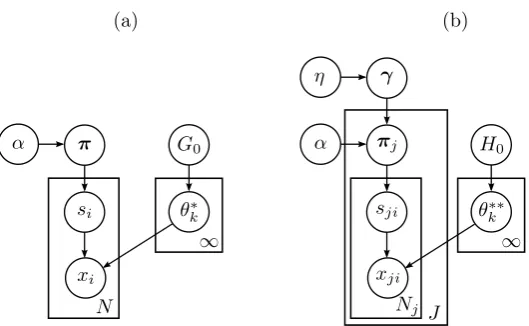
s�. The DPM model is depicted as a graphical
model in Figure 1(a).
The Hierarchical Dirichlet Process
In order to link group-specific DPs, Teh et al. (2006) introduced the hierarchical Dirichlet process (HDP).3 Here, group-specific distributions are conditionally
inde-pendent given a common base distribution G0 and follow Gj ∼ DP(α� G0). The
common base distribution itself follows a Dirichlet process G0 ∼ DP(η� H0). The
2
The Kronecker delta is a function of two variables that is 1 if they are equal and 0 otherwise.
3
Figure 1: (a) DPM Model and (b) HDPM Model
HDP thus has three parameters: the base measureH0 and the concentration param-eters α and η. The common base distributionG0 varies around the prior H0 where the amount of variability is determined by η. The group-specific distributions Gj
deviate from G0 withα governing the amount of variability.
In order to derive a stick-breaking representation for the HDP, we first express the global measure G0 as:
G0=
∞
�
k=1 γkδθ∗∗
k � (10)
where �θ∗∗
k }
∞
k=1 represent a set of support points drawn i.i.d. from H0 and γ =
�γk}∞k=1 ∼Stick(η). The Gj reuse the same support points as G0 but with different
proportions:
Gj=
∞
�
k=1
πjkδθ∗∗
k . (11)
The weights πj = �πjk}
∞
k=1 are independent given γ (since the Gj are independent
given G0) and one can show that πj ind
∼ DP(α�γ).
Teh et al. (2006) also develop a P´olya urn scheme for the HDP and we refer to their paper for technical details on this. The underlying analogue to the CRP is the
[image:7.595.164.429.100.263.2]proportionally to the number of tables (in the entire franchise) that have previously chosen that dish.
In order to derive thehierarchical Dirichlet process mixture model (HDPM model), we consider J groups of observations ��xji}
Nj
i=1}Jj=1 with xji ind
∼ F(θji). The
parame-ters�θji} Nj
i=1of thej-th group are generated from an unknown group-specific mixture
distribution Gj for which a HDP prior is assumed. Again, we can consider an
indi-cator variable representation of the HDPM model:
γ∼Stick(η) (12)
πj ind
∼ DP(α�γ)� j= 1� . . . � J� (13)
sji ∼πj� j= 1� . . . � J� i= 1� . . . � Nj� (14)
θ∗∗
k ∼H0� k = 1� . . . �∞� (15)
xji ind
∼ F(θ∗∗
sj�)� j= 1� . . . � J� i= 1� . . . � Nj� (16)
whereGj =
�∞
k=1πjkδθ∗∗
k andθji =θ
∗∗
sj�. The HDPM model is depicted as a graphical
model in Figure 1(b).
The Infinite Hidden Markov Model
The infinite hidden Markov model (IHMM) was introduced by Beal et al. (2002) and Teh et al. (2006). To get from the HDPM model to the IHMM (the IHMM is also referred to as the hierarchical Dirichlet process hidden Markov model, HDP-HMM), we start with a finitehidden Markov model (HMM). The HMM is a temporal probabilistic model where the state of the underlying process is determined by a single discrete random variable. More formally, we have an unobserved state sequence
s= (s1� . . . � sT) and a sequence of observationsy= (y1� . . . � yT). Each state variable
st can take on a finite number of distinct states: 1� . . . � K. Transitions between
the states are Markovian and parametrized by the transition matrix π with πij =
Pr (st=j|st−1=i). Each observation yt is conditionally independent of the other
observations given the state st with the corresponding likelihood depending on a
We can write the density ofyt given the previous state st−1 as:
p(yt|st−1=k) =
K
�
st=1
p(st|st−1=k)p(yt|st) =
K
�
st=1
πk�stp(yt|φst). (17)
We thus have a mixture distribution where the mixture weights πk =�πk�st}
K st=1 are
specified by st−1 = k and the mixture component generating yt is determined by
st. The HMM can thus be interpreted as a set of K finite mixture models, one for
each possible value of st−1. Expressed differently, each row of the transition matrix
π (indexed by st−1) specifies a different mixture distribution over the same set of
mixture components φ= (φ1� . . . � φK).
In order to derive a nonparametric version of the HMM with an unbounded set of states, we replace the finite mixture distributions with Dirichlet process mixtures, again one for each possibly visited state in the previous period. However, we need to couple the Dirichlet process mixtures in such a way that they share the same set of states. This can be done using a HDP mixture and we finally obtain the IHMM:
γ ∼Stick(η). (18)
πk∼DP(α�γ)� k= 1� . . . �∞� (19)
st ∼Multinomial(πst−1)� t= 1� . . . � T� s0 = 1� (20)
φk ∼H� k = 1� . . . �∞� (21)
yt ∼F(φst)� t= 1� . . . � T� (22)
The IHMM is shown as a graphical model in Figure 2 (for now, we ignoreκwhich will be introduced in the next section).
The Sticky IHMM
Figure 2: The infinite hidden Markov model (IHMM)
paper. Their idea is to increase the prior probability E(πkk) of a self-transition by
introducing a positive parameter κinto equation (19) which then becomes:
πk|α�γ� κ∼DP
�
α+κ�αγ+κδk α+κ
�
� k = 1� . . . �∞. (19*)
Thus, an amountκis added to thek-th component ofαγwhich leads to an increased probability of self-transitions. Note that the original IHMM can be obtained by setting κ= 0.
The metaphor that Fox et al. (2007, 2008) develop for their extended model is the CRF with loyal customers. Each restaurant now has a specialty dish that has the same index as the restaurant. This dish is served everywhere (since the restaurants still share the same buffet line) but is more popular in its namesake restaurant. In other words, each restaurant now has a specific rating of the buffet line that puts more weight on the specialty dish.
Hyperparameters and Prior Distributions
First, we must specify the distribution of the observations F(yt|φst) and the base
measureH. In our application to inflation dynamics we assume that the observations are normally distributed:
yt =x
�
tβst+εt� εt ∼N(0� σ 2
We then choose a normal-inverse gamma distribution as base measure:
βk|σk2∼N(b0� σk2�0)� σ2k ∼Inv-Gamma
� c0
2�
d0
2
�
� k= 1� . . . �∞. (24)
Note that the normal-inverse gamma distribution is conjugate which leads to straight-forward and efficient sampling of theβj andσj2. However, non-conjugate cases could
be handled as well with only minor modifications. We treat the hyperparameters
b0��0� c0� d0as fixed; another approach would be to place further prior distributions on them.
In contrast, the concentration parametersαandηand the self-transition parame-terκ are treated as unknown quantities which we learn from the data by performing full Bayesian inference. Fox et al. (2007, 2008) show that it is convenient not to work withα andκ directly but instead withα+κ and ρ=κ/(α+κ) and place the following prior distributions on them:
α+κ∼Gamma(e0� f0)� (25)
ρ∼Beta(g0� h0). (26) Finally, η is given a gamma prior:
η ∼Gamma(r0� s0). (27)
Inference via MCMC Sampling
Since the sticky IHMM is too complex to be analyzed analytically, we need to resort to MCMC sampling techniques (for a comprehensive survey on these methods see, for example, Robert and Casella, 2004). In principle, it is straightforward to set up a Gibbs sampler that alternates between drawing the state sequence, the parame-ters and the hyperparameparame-ters. However, a sampler that sequentially updates each state given all other state assignments generally mixes very slowly due to strong dependencies between consecutive time points.
One solution to this problem is to work with a finite approximation to the DP (Ish-waran and Zarepour, 2002) which is done in Fox et al. (2007, 2008). Another option is to follow Van Gael et al. (2008) who propose beam sampling for the IHMM. Their algorithm uses the concept of slice sampling (Neal, 2003) and is related to the ap-proach of Walker (2007) for DPM models. The basic idea is to augment the parameter space with a set of auxiliary variablesu= (u1� . . . � uT). These auxiliary variables do
not change the marginal distributions of the other variables but adaptively reduce the set of all valid state sequences to a finite one, such that dynamic programming techniques can be applied.
In our application, we use the beam sampling algorithm for drawing the state sequence. The Gibbs sampling steps for the parameters and hyperparameters are the same as in Fox et al. (2007, 2008). The complete MCMC sampling algorithm is described in the Appendix. For further details and derivations we refer to the original articles.
3
U.S. Inflation Dynamics
In this section we employ the sticky IHMM to analyze the dynamics of U.S. infla-tion. We measure the price level Pt using seasonally adjusted quarterly data on the
PCE deflator obtained from the Bureau of Economic Analysis. Annualized quarterly inflation is then calculated as πt = 400 ln(Pt/Pt−1). Our sample goes from 1953:I to
2009:III and we use earlier data to initialize the lags of our model.4
The inflation series is plotted in Figure 3. Starting out low, inflation rose during the 1970s, reaching a first peek at 11.7� in 1974 and a second peek at 11.8� in 1980. Then, the restrictive monetary policy of the Federal Reserve under Paul Volcker suc-ceeded in lowering inflation to 2.6� in 1983. Afterwards, the inflation rate remained rather stable, with the exception of 2008, when it experienced a sharp drop during the recent banking crisis.
Table 1 includes summary statistics for five different periods of the overall sample. The first-order autocorrelation, which gives us a first indication on the persistence of inflation, was rather low before 1965. During the subsequent 20 years, it was much higher, but declined again after 1985. In the end it was even lower than at the start
4
1955 1965 1975 1985 1995 2005
−
5
0
5
[image:13.595.144.432.121.351.2]10
Figure 3: U.S. Inflation Dynamics
of the sample.
As stated above, we assume that inflation is normally distributed and choose to work with a 4th-order autoregressive (AR) representation. Equation (23) becomes
πt =β0�st+ 4 �
i=1
βi�stπt−i+εt� εt ∼N(0� σs2t)� t= 1� . . . � T. (23*)
Thus, yt = πt, xt = (1� πt−1� . . . � πt−4) and βst = (β0�st� β1�st� . . . � β4�st). We use the
Period 1953:I 1965:I 1975:I 1985:I 1995:I - 1964:IV - 1974:IV - 1984:IV - 1994:IV - 2009:III Mean 1.489 4.533 6.420 3.223 2.049 S.D. 1.144 2.651 2.380 1.217 1.529 Autocorrelation 0.359 0.825 0.747 0.447 0.250
[image:13.595.110.480.544.623.2]prior distributions stated in equations (24) - (27) and choose the prior parameters in the following way. We set b0 = 0 and assume �0 to be diagonal with the prior
variance of the intercept equal to 5 and the prior variances of the AR coefficients equal to 1. Further, we setc0= 5 andd0= 3, which implies thatσ2
j has a prior mean
of 1.0 and a prior variance of 2.0. The prior distributions for the hyperparameters are assumed to be rather uninformative: e0= 125, f0 = 5, g0 = 10, h0 = 1, r0 = 5,
s0 = 1. Our results are based on every 50-th of 500,000 samples from the MCMC output after a burn-in period of 50,000 iterations.5
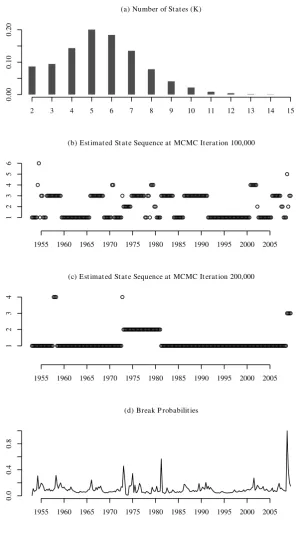
A histogram of the number of inferred states is shown in the top panel of Figure 4. The posterior mode is 5, but we see that the MCMC sampler averages over a large set of values ranging from 2 to 15. The middle two panels of Figure 4 show estimates of the state sequence at two randomly picked iterations of the MCMC sampler. In panel (b), which shows the estimates at iteration 100,000, the sequence consists of 6 different states, in panel (c), which gives the estimates at iteration 200,000, of 4 states. However, not only the numbers of states differ but also the patterns of the sequences. In panel (b) most observations belong to either state 1 or 3, and the sequence switches rather often between these two states. In panel (c), most observations are in state 1 or in state 2, and the sequence switches only once from state 1 to state 2 and once back. This example shows that the data are not overly informative about the actual state pattern. Therefore, it is very important to employ a flexible framework like the IHMM in modeling. The two estimated state sequences also demonstrate the IHMM’s capability of dealing with outliers. In panel (b), the observations at 1954Q3 and 2008Q4 are identified as outliers, each being the only observation in the respective state. Similarly, only a few observations occupy states 3 and 4 in panel (c).6 Finally, the bottom panel of Figure 4 shows posterior
means of the break probabilities Pr(st �=st−1). The three peaks are dated 1973Q1,
where we have a posterior break probability of 0.458, 1981Q2 with a posterior break probability of 0.567 and 2008Q4 with a posterior break probability of 0.998.
Figure 5 displays posterior means and 10� and 90� quantiles for the intercept, the variance and the sum of the AR coefficients �4i=1βi�st. The latter serves as
5
The algorithm is coded in C++. It takes around 30 minutes to draw 550,000 samples using a 3 GHz Intel �R) Core �TM) 2 Quad processor �employing a non-parallelized version of the code).
6
our measure of persistence.7 The intercept displays some variablities around 1975
and at the end of the sample, otherwise, it stays rather constant. However, the credible interval is rather wide. The variance is more fluctuating, being highest between 1973Q2 and 1981Q1. However, the credible set is very wide as well, and we cannot rule out a constant variance level. Finally, the sum of the AR coefficients is highest between 1973Q1 and 1974Q1 and between 1976Q4 and 1981Q1. Our measure of persistence displays a clear structural break during the recent banking crisis. Furthermore, the 90� posterior quantile always stays close to 1, and the credible set includes 1 at 38� of the points in the sample period. These results lead to the conclusion that, with the exception of the end of the sample, inflation persistence was high and nearly constant. However, the credible interval is very wide. Therefore, a considerable amount of uncertainty about the exact properties of inflation persistence remains.
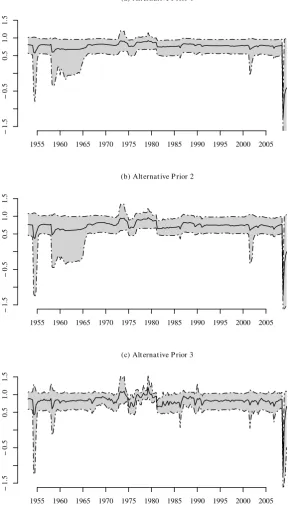
Figure 6 presents the outcome of a prior sensitivity analysis focusing on inflation persistence. We argued above that our main results are based on rather uninformative priors for the hyperparameters. In order to verify this, we employed three more informative priors, each of them changing one pair of hyperparameters compared to the prior used in the main analysis. First, we setr0 = 100 ands0= 10. This forcesη
to be higher and, thus, leads to a global transition distributionγ that is not as sparse as the original one. The top panel shows posterior means and 10� and 90� quantiles for the sum of the AR coefficients under this prior. Comparing these results with our main results in Figure 5(c), we see that they are nearly the same. The results do not change much either if we force α+κ to be higher by settinge0= 1000 and f0 = 25 (see the panel in the middle). Finally, we set g0 =h0 = 5, which implies a smaller number of self-transitions. The result is shown in the bottom panel. We see that inflation persistence is more bumpy, and the credible intervals are slightly narrower. However, the main conclusions about the properties of inflation persistence do not change.
7
4
Conclusions
We applied the infinite hidden Markov model (IHMM) to analyze U.S. inflation dynamics. The IHMM is a Bayesian nonparametric extension of the hidden Markov model (HMM). This means it does not fix the number of states a priori but learns it from the data. Thus, the IHMM is a convenient and flexible approach to model economic time series allowing for an unknown number of structural breaks.
(a) Number of States (K)
2 3 4 5 6 7 8 9 10 11 12 13 14 15
0.
00
0.
10
0.
20
(b) Estimated State Sequence at MCMC Iteration 100,000
1955 1960 1965 1970 1975 1980 1985 1990 1995 2000 2005
1
2
3
4
5
6
(c) Estimated State Sequence at MCMC Iteration 200,000
1955 1960 1965 1970 1975 1980 1985 1990 1995 2000 2005
1
2
3
4
(d) Break P robabilities
1955 1960 1965 1970 1975 1980 1985 1990 1995 2000 2005
0.
0
0.
4
0.
8
[image:17.595.142.439.115.653.2](a) Intercept
1955 1960 1965 1970 1975 1980 1985 1990 1995 2000 2005
−
1
0
1
2
3
(b) Variance
1955 1960 1965 1970 1975 1980 1985 1990 1995 2000 2005
0.
0
0.
5
1.
0
1.
5
2.
0
2.
5
(c) Sum of AR Coefficients
1955 1960 1965 1970 1975 1980 1985 1990 1995 2000 2005
−
1.
5
−
0.
5
0.
5
1.
0
1.
[image:18.595.142.435.101.645.2]5
(a) Alternative P rior 1
1955 1960 1965 1970 1975 1980 1985 1990 1995 2000 2005
−
1.
5
−
0.
5
0.
5
1.
0
1.
5
(b) Alternative P rior 2
1955 1960 1965 1970 1975 1980 1985 1990 1995 2000 2005
−
1.
5
−
0.
5
0.
5
1.
0
1.
5
(c) Alternative P rior 3
1955 1960 1965 1970 1975 1980 1985 1990 1995 2000 2005
−
1.
5
−
0.
5
0.
5
1.
0
1.
[image:19.595.146.437.126.646.2]5
References
Ang, A., Bekaert, G., 2002. Regime switches in interest rates. Journal of Business & Economic Statistics, 20, 163–182.
Beal, M., Krishnamurthy, P., 2006. Gene expression time course clustering with countably infinite hidden Markov models. Proceedings of the Conference on Un-certainty in Artificial Intelligence.
Beal, M. J., Ghahramani, Z., Rasmussen, C. E., 2002. The infinite hidden Markov model. Advances in Neural Information Processing Systems 14, 577–584.
Bernardo, J. M., Smith, A. F. M., 1994. Bayesian Theory. Wiley, New York.
Blackwell, D., MacQueen, J., 1973. Ferguson distributions via P´olya urn schemes. The Annals of Statistics 1, 353–355.
Brainard, W., Perry, G., 2000. Making policy in a changing world. In: Perry, G., Tobin, J. (Eds.), Economic Events, Ideas, and Policies: The 1960s and After. Brookings Institution Press, Washington.
Chib, S., 1998. Estimation and comparison of multiple change point models. Journal of Econometrics 86, 221–241.
Clements, M. P., Hendry, D. F., 1999. Forecasting Non-Stationary Economic Time Series. MIT Press, Cambridge, MA.
Cogley, T., Sargent, T. J., 2001. Evolving post-world war II U.S. inflation dynamics. NBER Macroeconomics Annual 16, 331–373.
Ferguson, T. S., 1973. A Bayesian analysis of some nonparametric problems. The Annals of Statistics 1, 209–230.
Fox, E. B., Sudderth, E. B., Jordan, M. I., Willsky, A. S., 2007. The sticky HDP-HMM: Bayesian nonparametric hidden Markov models with persistent states. Tech. Rep. 2777, MIT Laboratory for Information and Decision Systems.
Giordani, P., Kohn, R., van Dijk, D., 2007. A unified approach to nonlinearity, structural change, and outliers. Journal of Econometrics 137, 112–133.
Ishwaran, H., Zarepour, M., 2002. Exact and approximate sum-representations for the Dirichlet process. The Canadian Journal of Statistics 30, 269–283.
Kivinen, J. J., Sudderth, E. B., Jordan, M. I., 2007. Learning multiscale repre-sentations of natural scenes using Dirichlet processes. Proceedings of the IEEE International Conference on Computer Vision.
Koop, G., Potter, S., 2001. Are apparent findings of nonlinearity due to structural instability in economic time series? The Econometrics Journal 4, 37–55.
Koop, G., Potter, S., 2007. Forecasting and estimating multiple change-point models. Review of Economic Studies 74, 763–789.
Neal, R. M., 2003. Slice sampling. Annals of Statistics 31, 705–741.
Nelson, C. R., Schwert, G. W., 1977. Short-term interest rates as predictors of infla-tion: On testing the hypothesis that the real rate of interest is constant. American Economic Review 67, 478–486.
Pitman, J., 2006. Combinatorial Stochastic Processes. Springer, Berlin.
Pivetta, F., Reis, R., 2007. The persistence of inflation in the United States. Journal of Economic Dynamics and Control 31, 1326–1358.
Rabiner, L. R., 1989. A tutorial on hidden Markov models and selected applications in speech recognition. Proceedings of the IEEE 77, 257–286.
Robert, C. P., Casella, G., 2004. Monte Carlo Statistical Methods. Springer, New York.
Sethuraman, J., 1994. A constructive definition of Dirichlet priors. Statistica Sinica 4, 639–650.
Stock, J. H., 2001. Evolving post-world war II U.S. inflation dynamics: Comment. NBER Macroeconomics Annual 16, 379–387.
Stock, J. H., Watson, M. W., 2007. Why has U.S. inflation become harder to forecast? Journal of Money, Credit and Banking 39, 3–33.
Taylor, J., 1998. Monetary policy guidelines for unemployment and inflation stability. In: Friedman, B., Solow, R. (Eds.), Inflation, Unemployment and Monetary Policy. MIT Press, Cambridge.
Taylor, J., 2000. Low inflation, pass-through, and the pricing power of firms. Euro-pean Economic Review 44, 13891408.
Teh, Y. W., Jordan, M. I., 2010. Hierarchical Bayesian nonparametric models with applications. In: Hjort, N. L., Holmes, C., M¨uller, P. (Eds.), Bayesian Nonpara-metrics. Cambridge University Press, Cambridge.
Teh, Y. W., Jordan, M. I., Beal, M. J., Blei, D. M., 2006. Hierarchical Dirichlet processes. Journal of the American Statistical Association 101, 1566–1581. Van Gael, J., Saatci, Y., Teh, Y. W., Ghahramani, Z., 2008. Beam sampling for the
infinite hidden Markov model. Proceedings of the 25th International Conference on Machine Learning.
Appendix: Implementation of the MCMC Sampler
This Appendix gives details on the MCMC sampler which combines the beam sam-pling algorithm of Van Gael et al. (2008) with the samsam-pling techniques for the sticky IHMM derived in Fox et al. (2007, 2008). The parameters that need to be sampled are the hyperparameters η,α and κ, the global transition distribution γ, the transi-tion distributransi-tions π =�πk}Kk=1, the state sequences=�st}Tt=1, and the parameters
of the outcome distributions θ = �βk� σ2k}Kk=1. K denotes the number of distinct
states (which are labeled 1� . . . � K) and changes during sampling. The auxiliary vari-ables u =�ut}Tt=1 are introduced to make the set of possible state sequences finite.
Another set of auxiliary variables consists of m = ��mjk}Kj=1}Kk=1, where (in terms
of the Chinese restaurant franchise) mjk denotes the number of tables in restaurant
j that were served dish k, r = �rk}Kk=1, where rk denotes the number of tables in
restaurant k that eat the namesake dish k but originally considered to eat another dish (and finally were overridden due to the increased probability of a self-transition), and m = ��mjk}Kj=1}Kk=1, where mjk denotes the number of tables in restaurant j
that considered to eat dishk. The auxiliary variablesv =�vk}Kk=1,w=�wk}Kk=1,ν,
and λare helpful for sampling the hyperparameters. Finally,njk counts the number
of transitions from j to k in the state sequence s. Sums are denoted by dots, i.e.
x∙b=
�
axab,xa∙=
�
bxab, andx∙∙=
�
b
�
axab. The MCMC sampler then consists
of the following steps:
(0) Initialize parameters: Choose a starting value for K and initialize all parameters. The infinitely many states that do not occur insare merged into one state. Thus γ and each πk haveK+ 1 elements.
(1) Samplingu: Fort= 1� . . . � T, sampleut fromϕ(ut|π� st−1� st) = U(0� πst−1st),
where U(a� b) denotes the uniform distribution on the interval (a� b). (2) Sampling s:
(i) If necessary, breakπ andγ: While max(�πk�K+1}kK=1)>min(�ut}Tt=1),
repeat the following steps: (a) DrawπK+1∼Dirichlet(αγ).
(b-1) Drawζ ∼Beta(1� η).
(b-2) Add element γK+2= (1−ζ)γK+1 .
(b-3) Set γK+1=ζγK+1.
(c) Break the last element of eachπk. For k= 1� . . . � K+ 1:
(c-1) Drawζk ∼Beta(αγK+1� αγK+2).
(c-2) Add elementπk�K+2 = (1−ζk)πk�K+1.
(c-3) Set πk�K+1 =ζkπk�K+1.
(d) Sampleσ2
K+1∼Inv-Gamma �c0
2�
d0 2 �
and βK+1∼N(b0� σK2+1�0).
(e) IncrementK.
(ii) Sample s: Samples fromϕ(s|π�u�θ):
(a) Working sequentially forward in time, calculate
mt(k) = P(y1� . . . � yt|st=k�u):
(a-1) Initializem1(k) = 1(u1< π1k)N(y1|x�1βk� σ2k) fork = 1� . . . � K.
(a-2) Induce mt(k) =
�K
l=11(ut < πlk)N(yt|x
�
tβk� σk2)mt−1(l)
for t= 2� . . . � T and k = 1� . . . � K.
(b) Working sequentially backwards in time, sample state indicators: (b-1) Sample sT from
�K
k=1mT(k)δ(st� k).
(b-2) Sample st from�Kk=1mt(k)δ(st� k)1(ut+1< πk�st�1)
for t=T −1� . . . �1.
(3) Cleaning up: Remove the redundant states and relabel the remaining ones from 1� . . . � K. Adaptγ,π,β, and σ2 accordingly.
(4) Sampling auxiliary variables m, r and m:
(i) Sample m: For j = 1� . . . � K and k = 1� . . . � K, sample mjk from
ϕ(mjk|s� γk� α� κ) as follows: Set mjk = 0. For i = 1� . . . � njk, sample
xi ∼Bernoulli
�
αγk+κδ�j�k)
i−1+αγk+κδ�j�k)
�
.Ifxi= 1 increment mjk.
(ii) Sample r: Forj= 1� . . . � K, sample rj from
ϕ(rj|mjj� γj� α� κ) = Binomial
�
mjj�ρ+γjρ�1−ρ)
�
, where ρ= κ α+κ.
(iii) Update m: For j= 1� . . . � K and k = 1� . . . � K, set mjk =mjk ifj�=k,
(5) Sampling γ: Draw γ fromϕ(γ|m� η) = Dirichlet(m∙1� . . . �m∙K� η).
(6) Sampling π: Fork = 1� . . . � K, sample πk from
ϕ(πk|γ�s� α� κ) = Dirichlet(αγ1+nk1� . . . � αγk+κ+nkk� . . . � αγK+nkK� αγK+1).
(7) Sampling θ: Fork= 1� . . . � K, sampleσ2
k ∼Inv-Gamma
�c ∗ 2� d∗ 2 �
andβK+1 ∼
N(b∗� σ2K+1�∗) with�∗= (B −1
0 + �
t:st=kxtx
�
t)
−1
,b∗=�∗(� −1
0 b0+�t:st=kxtyt),
c∗=c0+
�
t:st=k1 and d∗=d0+s2+ ( ˆβ−β∗) �
(�
t:st=kxtx
�
t)�∗� −1
0 ( ˆβ−β∗),
where ˆβ = (�
t:st=kxtx
�
t)
−1�
t:st=kxtyt and s2=
�
t:st=k(yt−x
�
tβˆ)2.
(8) Sampling hyperparameters α, κ and η:
(i) Sample α+κ:
(a) Fork = 1� . . . � K, samplevkfromϕ(vk|α+κ�s) = Bernoulli
�
nk∙
nk∙+α+κ
�
. (b) Fork = 1� . . . � K, samplewkfromϕ(wk|α+κ�s) = Beta (α+κ+ 1� nk∙).
(c) Sampleα+κfrom
ϕ(α+κ|v�w�m) = Gamma�e0+m∙∙−
�K
k=1vk� f0−
�K
k=1logwk
�
. (ii) Sample ρ: Draw ρfrom ϕ(ρ|m�r) = Beta(g0+r∙� h0+m∙∙−r∙).
(iii) Calculate α and κ: Setα= (1−ρ)(α+κ) andκ =ρ(α+κ). (iv) Sample η:
(a) Sampleν from ϕ(ν|η�m) = Bernoulli� �
∙∙
�∙∙+η
�
. (b) Sampleλfromϕ(λ|η�m) = Beta(η+ 1�m∙∙).
(c) Sampleηfromϕ(η|λ� ν�m) = Gamma�
r0+K−ν� s0−logλ�
, where
K=�K
k=11(m∙k>0).