Sanchez, J.P. and McInnes, C.R. (2010) Assessment on the feasibility of
future shepherding of asteroid resources. In: 61st International
Astronautical Congress, IAC 2010, 2010-09-27 - 2010-10-01. ,
This version is available at
https://strathprints.strath.ac.uk/27784/
Strathprints is designed to allow users to access the research output of the University of Strathclyde. Unless otherwise explicitly stated on the manuscript, Copyright © and Moral Rights for the papers on this site are retained by the individual authors and/or other copyright owners. Please check the manuscript for details of any other licences that may have been applied. You may not engage in further distribution of the material for any profitmaking activities or any commercial gain. You may freely distribute both the url (https://strathprints.strath.ac.uk/) and the content of this paper for research or private study, educational, or not-for-profit purposes without prior permission or charge.
Any correspondence concerning this service should be sent to the Strathprints administrator: [email protected]
The Strathprints institutional repository (https://strathprints.strath.ac.uk) is a digital archive of University of Strathclyde research outputs. It has been developed to disseminate open access research outputs, expose data about those outputs, and enable the
Page 1 of 15 ASSESSMENT ON THE FEASIBILITY OF FUTURE SHEPHERDING OF ASTEROID RESOURCES
J.P. Sanchez
Advanced Space Concepts Laboratory, University of Strathclyde, UK, [email protected]
C.R. McInnes
Advanced Space Concepts Laboratory, University of Strathclyde, UK, [email protected]
Most plausible futures for space exploration and exploitation require a large mass in Earth orbit. Delivering this mass requires overcoming the Earth’s natural gravity well, which imposes a distinct obstacle to any future space venture. An alternative solution is to search for more accessible resources elsewhere. In particular, this paper examines the possibility of future utilisation of near Earth asteroid resources. The accessibility of asteroid material can be estimated by analysing the volume of Keplerian orbital element space from which Earth can be reached under a certain energy threshold and then by mapping this analysis onto an existing statistical near Earth asteroid (NEA) model. Earth is reached through orbital transfers defined by a series of impulsive manoeuvres and computed using the patched-conic approximation. The NEA model allows an estimation of the probability of finding an object that could be transferred with a given ∆v budget. For the first time, a resource map provides a realistic assessment of the mass of material resources in near Earth space as a function of energy investment. The results show that there is a considerable mass of resources that can be accessed and exploited at relatively low levels of energy. More importantly, asteroid resources can be accessed with a entire spectrum of levels of energy, unlike other more massive bodies such as the Earth or Moon, which require a minimum energy threshold implicit in their gravity well. With this resource map, the total change of velocity required to capture an asteroid, or transfer its resources to Earth, can be estimated as a function of object size. Thus, realistic examples of asteroid resource utilisation can be provided.
ost of the plausible futures for human space exploration and exploitation involve a large increase of mass in Earth orbit. Some examples include space solar power, space tourism or more visionary human space settlements. Whether this mass is water for crew, propellant for propulsion or materials for structures, these resources will require overcoming Earth’s natural gravity well to be delivered in space. Thus, even if technologically possible, this will certainly put a large economic burden on future space progress. An alternative to this approach is to search among the population of asteroids in search of the required reservoir of material[1-2].
Asteroids are of importance in uncovering the formation, evolution and composition of the solar system. In particular, near Earth asteroids (NEA) have risen in prominence because of two important points: they are among the easiest celestial bodies to reach from the Earth and they may represent a long-term threat[3]. The growing interest in these objects has translated into an increasing number of missions to NEA, such as the sample return missions Hayabusa[4] and Marco Polo[5],
impactor missions such as Deep Impact* and possible
deflector demonstrator missions such as Don Quixote†.
*http://www.nasa.gov/mission_pages/deepimpact/ma
in/index.html
†http://www.esa.int/SPECIALS/NEO/SEMZRZNV
GJE_0.html
With regard to asteroid deflection, a range of methods have been identified to provide a change in the asteroid linear momentum[6]. Some of these methods, such as the kinetic impactor have been deemed to have a high technology readiness level (TRL), while others may require considerable development. If the capability to impact an asteroid exists (e.g., Deep Impact), or if the capability to deflect an asteroid is available in the near future, a resource-rich asteroid could in principle be manoeuvred and captured into a bound Earth orbit through judicious use of orbital dynamics. On the other hand, if direct transfer of the entire NEA is not possible, or necessary, extracted resources could also be transferred to a bound Earth orbit for utilisation. It is envisaged that NEA could also be ‘shepherded’ into easily accessible orbits to provide future resources.
Page 2 of 15 asteroid population. The resulting resource map
provides an accurate assessment of the real material resources of near Earth space as a function of energy investment. It will be shown that there are substantial materials resources available at low energy based on the statistical distribution of near Earth asteroids.
The population of near-Earth objects is modelled in this paper by means of an object size distribution together with an orbital element distribution function. The size distribution is defined via a power law relationship between the asteroid diameter and the total number of asteroids with size lower than this diameter[7]. On the other hand, the orbital distribution used in this paper will rely on Bottke et al.[8] asteroid model to estimate the probability to find an object with a given set of Keplerian elements.
The dynamic model used to study the Keplerian orbital element space {a,e,i} of asteroid-to-Earth transfers assumes a circular Earth orbit with a 1 AU semi-major axis. The Sun is the central body for the motion of the asteroid, and the Earth’s gravity is only considered when the NEA motion is in close proximity. Since the orbital transfers will be modelled as a series of impulsive changes of velocity, for some conditions, analytical formulae relate the total change of velocity with the region of Keplerian space that can be reached.
Two different transfer models are included in this paper. Firstly, a phase-free two-impulse transfer, which is composed of a change of plane manoeuvre and a perigee capture manoeuvre at Earth encounter. This transfer, as with a Hohmann transfer analysis, provides a good conservative estimate of the exploitable asteroid material. Secondly, a phase-free one-impulse transfer, which only considers a perigee capture manoeuvre during the Earth fly-by. In this second case, only orbits that have initially very low Minimum Orbital Intersection Distances (MOID) can be captured. The MOID is the minimum possible distance between the Earth and the asteroid considering free-phasing for both objects. Finally, an estimation of the phasing manoeuvre required to meet the Earth at the orbital intersections will also be included on the transfer sequence.
II. NEAR EARTH ASTEROIDS
By convention, a celestial body is considered a Near Earth Object (NEO) if its perihelion is smaller than 1.3 AU and its aphelion is larger than 0.983 AU. This is a very broad definition which includes predominantly asteroids, but also a small percentage of comets. NEOs are then the closest celestial objects to the Earth and therefore the obvious first targets for any resource exploitation mission (excluding the Moon).
The first NEA (Near-Earth Asteroid) was discovered in 1898 (433 Eros) and since then more than 7000 asteroids have been added to the NEO catalogue. Most of these objects have been surveyed during the last 20 years as a consequence of the general recognition of the impact threat that these objects pose to Earth [9]. This recognition led to a series of efforts to catalogue 90% of objects with the potential to pose a global environmental threat [10] (i.e., Diameter>1km). Subsequent recommendations suggested to pursue 90% completeness of the census of 140-m objects by 2020 [7]. The new generation of surveys such as LSST [11] or Pan-STARRS [12] are well positioned to achieve this objective.
Together with the ever-growing catalogue of asteroids, the understanding of the origin and evolution of these objects has seen enormous advancements in recent years [13]. Still, it is not possible to know accurately the amount and characteristics of asteroid exploitable resources. However, reliable order of magnitude estimates may now provide some insight concerning the feasibility of future space resource exploitation and utilisation concepts (e.g., space-based climate engineering[14]).
In order to determine near-Earth resource availability, a sound statistical model of the near Earth asteroid population is required. The following sections will describe an asteroid model of the fidelity necessary to allow the order of magnitude analysis. The asteroid model described is composed of two parts; a size population model, which describes the net number of asteroids as a function of object size and an orbit distribution model that describes the likelihood that an asteroid will be found in a given region of orbital element space.
II.I Near Earth Asteroid Population
The NEA size distribution is taken from the Near-Earth Object Science Definition report[7]. It is based on the results of a substantial number of studies estimating the population of different ranges of object sizes by a number of techniques (see
Fig. 1 taken from Stokes et al. [7]). The Near-Earth Object Science Definition report provides an accumulative population of asteroids that can be expressed as a constant power law distribution function of object diameter as:
( [ ]) b
N D km CD (1)
Page 3 of 15 Fig. 1: Accumulative size distribution of Near Earth
Objects (from Stokes et al. [7]).
Assuming a population of asteroids defined by a power law distribution such as Eq.(1), one can easily calculate the total number of objects within an upper and lower diameter range:
min max
min max
b b
N D D D C D D
(2)
where Dmax and Dmin are the maximum and minimum
diameter chosen. An estimation of the total asteroid mass composed by all these objects can also be computed. To do so, the following integration needs to be performed:
min max min
max
[ ] [ ]
D
D N
N
D D D km
M
m dN
(3)where m is the mass of the asteroid and
min
D N and
max
D
N are the number of objects bigger than Dmin and
Dmax respectively.
Assuming that all asteroids have a spherical shape and an average densitya, the mass m of the asteroid
can be defined by
36 a D
and the integration can
be defined as an integration over the asteroid diameter:
min max min
max
3
[ ] 6 a
D
D D
D
dN
D dD
dD
M
(4)where dN dD is the derivative of Eq.(1) with respect
the diameter D. Integrating Eq.(4), the total mass of asteroid material composed of asteroids with diameters between Dmax and Dmin results in:
max min
3 3
max min
[ ] 6 3
b b
a
D D
C b D D
b
M
(5)The average asteroid densityacan be approximated as 2600 kg/m3 (ref.[15]). Thus, for example, Eq.(5) can yield the total mass of “Tunguska” size objects (i.e.,
from 50 m to 70 m diameter) in near Earth space as being in the order of 1014 kg[16]. More recent estimates of the population of small asteroids [10] seem to indicate a possible drop by a factor of 2/3 on the estimations given by Eq.(1) for small objects between 10 to 500 meters diameter. Final results and discussion will also account for this possibility.
Finally, if the maximum diameter is set equal to the largest near Earth object known, 1036 Ganymed, which is 32 km in diameter and the minimum object size is set at 1 meters diameter, then Eq. (5) yields a total mass of 4.38x10¹⁶ kg. Note that the mass of a 32-km diameter spherical object with a density of 2600 kg/m3 is already higher than the estimation yielded by Eq.(5). The reason for this is that the power law distribution (1) underestimates the number of large objects existing. Nevertheless, this result will be taken as the estimated total mass of asteroid material available in near Earth orbit space. Now, it is necessary to define the energy requirements for transporting this material to Earth orbit in order to draw conclusions concerning practical resource availability.
II.II Near Earth Asteroid Orbital Distribution
This section describes the NEA orbital distribution model used to estimate the likelihood of finding an asteroid within a given volume of Keplerian orbital element space
a, e, i, , , M
. This likelihood can also be interpreted as the fraction of asteroids within the specified region of the Keplerian space, and thus, if multiplied by Eq.(5), results in the portion of asteroid mass within that region. Hence, the ability to calculate this likelihood, together with the ability to define the regions of the Keplerian space from which the Earth can be reached with a given ∆v budget, will later allow us to compute the asteroid resources available in near-Earth space.The NEA orbital distribution used here is based on an interpolation from the theoretical distribution model published in Bottke et al.[8]. The data used was very kindly provided by W.F. Bottke (personal communication, 2009). Bottke et al.[8] built an orbital distribution of NEA by propagating in time thousands of test bodies initially located at all the main source regions of asteroids (i.e., the 6 resonance, intermediate
source Mars-crossers, the 3:1 resonance, the outer main belt, and the trans-Neptunian disk). By using the set of asteroids discovered by Spacewatch at that time, the relative importance of the different asteroid sources could be best-fitted. This procedure yielded a steady state population of near Earth objects from which an orbital distribution as a function of semi-major axis a, eccentricity e and inclination i can be interpolated numerically.
Page 4 of 15 periapsis and the mean anomaly M, are assumed here
to be uniformly distributed random variables. The ascending node and the argument of periapsis are generally believed to be uniformly distributed in near Earth orbit space[17] as a consequence of the fact that the period of the secular evolution of these two angles is expected to be much shorter than the life-span of a near Earth object[18]. Therefore, we can assume that any value of and is equally possible for any NEA. All
values of mean anomaly M are also assumed to be
equally possible, and thus M is also uniformly
distributed between 0 to 2 .
[image:5.595.74.292.425.548.2]A probability density function
a e i, ,
has been created by linearly interpolating a 3-dimensional set of data containing the probability density at semi-major axes ranging from 0.05 to 7.35 AU with a partition step size of 0.1 AU, eccentricity ranging from 0.025 to 0.975 with a partition step of 0.05 and inclination ranging from 2.5 to 87.5 deg with a partition step of 5 deg. When
a e i, ,
requires a value outside the given grid of points (e.g., inclination less than 2.5 degrees) then a nearest neighbour extrapolation is used for the dependence on semi-major axis and eccentricity, while a linear extrapolation is used for the dependence on inclination. Fig. 2 shows both the
a e i, ,
projected in the {a,e} plane and the Aten, Apollo and Amor regions.Fig. 2: Bottke et al.[8] probability distribution built as an interpolation from the model data projected in the {a,e} plane.
Finally, an integration such as:
max max max
min min min
, ,
a e i
a e i
P
a e i di de da (6)will then yield the probability of finding an asteroid within the Keplerian elements defined by [amax,amin],
max min
[e ,e ] and [imax,imin]. Section III will later describe how these limits can be defined as a function of the delta-velocity budget for different transfer types.
III. ASTEROID MATERIAL TRANSFER This section will now describe the methodology followed to estimate the cost of transporting asteroid
material to Earth. Two different scenarios are envisaged; the transport of mined material and the transport of the entire asteroid. The first scenario, the transport of mined material, requires less energy to transport resources, since less mass is transported to Earth orbit, while requires that the mining operations occur in-situ. The latter requirement results in either very long duration manned missions, with the complexity that this entails, or, if the mining is performed robotically, the need for advanced autonomous systems due to both the communication delay between asteroid and Earth and the complexity of mining operations. The second scenario, on the other hand, requires moving a large mass, with the difficulty that this involves, but allows a more flexible mining on the Earth’s neighbourhood. The ultimate optimality of these two scenarios would depend on each particular asteroid (i.e., size and particular resources) and the future development of the key technologies required for such missions.
The analysis presented here focuses on the use of ∆v
as a figure of merit (FoM) for the transport cost. This is also a measure of the specific energy, i.e., energy per unit of mass, required to transport material to Earth and, therefore the two envisaged transportation scenarios can benefit from the same FoM to draw conclusions about the feasibility of a mission.
This section will first describe the two transfer models used. The first transfer assumes a two-impulse trajectory, which includes a change of plane and Earth insertion manoeuvre. While any Earth-crossing asteroid can be transferred to Earth using these two manoeuvres, some asteroids have orientations such that they can easily fly-by the Earth with an almost negligible phasing manoeuvre (i.e., asteroids with very low MOID). These objects could be captured with one single impulsive manoeuvre during the Earth passage. These two transfer models will be defined by using a patched conic approximation, thus, the motion of the asteroid, or any material resources extracted, would be dominated by the gravitational influence of the Sun, except when in a very close encounter with the Earth. The Earth is also assumed to be in a circular orbit with radius 1 AU.
Page 5 of 15 III.II Two-impulse transfer
The first impulsive manoeuvre in this capture sequence provides the change of plane necessary to make the asteroid orbit coplanar with the Earth. Using a more complex and realistic sequence of manoeuvres, a single combined manoeuvre could provide both the required phasing and the change of plane such that an Earth flyby occurs. In that case, the asteroid transfer to Earth would not need to be strictly coplanar with the Earth and the change of velocity necessary for the manoeuvre would be minimised. Unfortunately, this procedure would require a full numerical optimisation for each individual case, which would be unmanageable for the scope of this paper.
A simpler approach is to consider a change of plane manoeuvre such as:
2 sin( )
2 inc plX
i
v v
(7)
where vincis the impulsive change of velocity
necessary to change the orbital plane by ∆i, and vplX is the velocity of the asteroid at the Earth-orbital plane crossing. After thevincmanoeuvre, the magnitude of
the orbital velocity vplX remains the same, only the
inclination of the orbit has changed. Equation (7) allows a more analytical approach to the problem and at the same time provides a worst case scenario for the cost of the change of plane.
[image:6.595.82.286.443.566.2]Coplanar motion
Fig. 3: Orbital geometry of the coplanar model.
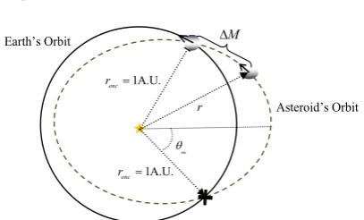
As shown in Fig. 3, an Earth-crossing coplanar asteroid has two intersections (points of MOID equal 0) with the Earth’s orbit. These are found when the asteroid is at 1 AU from the Sun. Since the distance r
from the Sun to the asteroid is known, the equation of the orbit in polar coordinates yields the true anomaly of the two encounters enc:
1 1
cos
enc
p e
(8)where 2
(1 )
pa e is the asteroid’s semi-latus rectum
and the unit length in Eq.(8), and any of the following formulas in this paper, has been normalized to 1 AU.
With the true anomaly of the encounter enc known, the velocity at the encounter can now be defined by using the normal and radial components of Keplerian orbital motion:
sinenc Sun
r enc
v e
p
(9)
1 cos
enc Sun
n enc
v e
p
(10)
where vrenc and enc n
v are the radial and normal velocity
at the MOID point. Using Eq. (8) and Eqs.(9)-(10), the encounter velocity can be rewritten in a more suitable form:
2 2
1
enc Sun r
v e p
p
(11)
enc
n Sun
v p (12)
Whenever the Earth-coplanar asteroid meets the Earth at enc, the velocity of the asteroid relative to the
Earth will then be
vrenc,
vnencrenc
with the Earth moving at an angular velocity Sun . This Earthencounter conditions will result on a hyperbolic motion of the asteroid relative to the Earth with an excess velocity as:
3
1
2
Sun
v
p
a
(13)Final Earth insertion
If MOID is zero or almost zero, the Earth encounter could be easily tuned by a phasing manoeuvre so that the altitude during the Earth fly-by is some given minimum distance (chosen here to be 200km) above the Earth’s surface. At this minimum altitude a final insertion manoeuvre could be performed.
The notion of targeting asteroids towards the Earth may raise some concerns with regards to a possible enhancement of the impact threat. Clearly, changing the orbit of a large NEA could potentially be a threat to Earth, although engineering the orbit of large objects may also be unfeasible. Thus for this objects transferring mined resources may provide the best and only option. On the other hand, for smaller bodies the impact hazard can be mitigated since bodies of tens of meters of diameter should completely ablate in the atmosphere[19]. Thus, bodies in the order of 10 meters diameter may be perfect targets for first capture demonstrator missions.
A parabolic orbit is assumed here to be the threshold between an Earth-bound orbit and an Earth escape orbit.
Hence, the ∆v necessary for an Earth capture vcap at
the perigee passage results in: Asteroid’s Orbit
1A.U.
enc
r
Earth’s Orbit M
1A.U.
enc
r
r
enc
Page 6 of 15
2
2 2
cap
p p
v v
r r
(14)
where v is the hyperbolic excess velocity described in
Eq.(13) and rp is the pericentre altitude (i.e.,r200km
). Finally, the sum of Eqs.(7) and (14) provides the total
∆v budget for a two-impulse transfer to Earth. Keplerian Feasible Regions
As noted earlier, the integration in Eq.(6) yields the probability of an asteroid to be found within a specified Keplerian region. By rearranging Eqs.(7) and (14), we can now define the regions from which transfers to Earth cost less than a given limit ∆vthr. Fig. 4, for
example, shows the Keplerian region in the plane {a,e} where asteroid resources can be transfer to Earth with a
total ∆v equal or lower than 2.37 km/s. This ∆v
[image:7.595.125.237.104.142.2]corresponds to the Moon’s escape velocity, thus offering a direct comparison between material available at the Moon and within an equivalent energy threshold elsewhere in the solar system. Also, superimposed in the figure are almost 5,000 asteroids (tiny dots and small crosses), which had been surveyed by April 2010.
Fig. 4: Keplerian {a,e} space reached by a maneuvre of 2.37 km/s (i.e., Moon’s escape velocity). Superimposed are all near Earth asteroids known within the {a,e} space as of April 2010.
Fig. 4 shows three different lines (solid, dash-dotted and dotted line) delimiting an area in the {a,e} plane. The solid line results from expressing Eq.(14) as an explicit function of the semi-major axis a and vcap
necessary for an Earth capture:
2 21 1
, 1 3
4
cap
s v
e v a
a a
(15)
where the hyperbolic excess velocity v∞ is defined as: 2
2 2
p p
cap
v
r r
v
(16)Equation (15) therefore yields the value of eccentricity for which an asteroid with semi-major axis
a can be captured with a manoeuvre ∆vcap at the perigee
passage. Asteroids with semi-major axis a, but
eccentricity lower than the result provided by Eq.(15) should be captured with a manoeuvre lower than vcap.
Thus, if vcapis set to the maximum allowed
manoeuvre ∆vthr, the eccentricity resulting from Eq.(15)
is also the maximum allowed eccentricity,
max thr,
e e v a , i.e., solid line in Fig. 4 when
∆vthr=2.37 km/s.
Eccentricities lower than emax require lower ∆v
manoeuvres to be captured at the Earth, but there is a geometrical limit to the minimum Earth insertion manoeuvrevcap.The minimum vcap occurs when the encounter geometry is such that the intersection is at the line of apsis. With this geometry only one intersection point exists, and lower eccentricities imply orbits with no Earth-crossing points (see Fig. 4). The minimum allowed eccentricity for an orbit with semi-major axis a
is therefore:
min
1 1 if 1
1 1 if 1
a a
e a
a a
(17)
so that, if a1,the periapis radius is 1 (see dotted line in Fig. 4), and, if instead a 1,the apoapsis is 1 (see dash-dotted line in Fig. 4).
Once the analytical expressions for the maximum and minimum eccentricity emax and emin are known, the
maximum and minimum allowed semi-major axis a can
be computed by finding when
max threshold
,
mine
v
a
ea
occurs. The latter equationresults in a second degree polynomial with the following two solutions:
min 2 2
max
1
1 2
threshold
s s
a v
v v
(18)
where v∞ is defined as in Eq.(16) and amin correspond to
the positive sign while amax corresponds to the negative.
Inside this delimited area within the {a,e} Keplerian space, we can ensure that the coplanar capture manoeuvres will be lower than the limit threshold ∆vthr.
Thus, the reminder impulse,
∆vinc(a,e,∆vthr)=∆vthr-∆vcap(a,e) , (19) can be used for changing the orbital plane of any available objects.
From Eq.(7) one can see that the cost of changing the orbital plane of a given asteroid is not only defined by the initial {a,e,i} of the asteroid, but also by the argument of the periapsis . The reason for this is that the velocity at the crossing plane vplX is the velocity at the line of nodes of the asteroid, whose orientation
-1 -0 .5 0 0.5 1
x
-3 5 -3 -2 5 -2 -1 5 -1 -0 5 0 0 5 1
max , threshold e a v
min
e a
-1-0.8-0.6-0.4-0. 200.20. 40. 60. 81
-1
0.8 0.6 0.4 0.2
0
0.2 0.4 0.6 0.8
[image:7.595.71.289.381.562.2]Page 7 of 15 within the orbit of the asteroid is defined by . Now, for
a given orientation, or specified , the optimal location for a change of plane is the furthest node from the Sun, since this corresponds to the lowest velocity, and therefore, minimises Eq.(7). This then concludes that the optimal orientation of an asteroid for changing its plane to an inclination of 0 degrees is such that the line of nodes is the line of apsis, while the worst orientation is such that the line of nodes is the semilatus rectum. Considering the worst orientation, the maximum inclination from which asteroids can be placed into a coplanar orbit is:
1
max_ 1/ 2
2
, ,
, , 2 sin
2 1
inc thr
p thr
S
v a e v
i a e v
e p (20)
Thus, any orbit with an inclination lower than imax_p, no
matter the orientation (i.e., ), has a two-impulse transfer to Earth with a ∆v budget lower than or equal to
∆vthr. The small crosses shown in Fig. 4 represent the
surveyed asteroids with inclinations lower than the resultant from Eq.(20).
Considering now the best possible orientation, where the change of plane manoeuvre occurs at the apoapsis, the maximum inclination from which asteroids can be placed into coplanar orbit is:
1
max_ 1/ 2
, ,
, , 2 sin
1 2 1 a inc thr r thr S
v a e v
i a e v
e a e (21)
Thus, any asteroid with an inclination higher than imax_ra,
no matter the orientation, cannot be transported to Earth with a ∆v budget lower than or equal to ∆vthr.
For inclinations between imax_p and imax_ra only a
fraction, between 0 and 1, of asteroids will statistically have the orientation required for a change of inclination within the ∆v budget. In order to compute this fraction, one can start by calculating the range of true anomalies that allow a change of plane within the required ∆v. A true anomaly allowing the change of plane refers to a true anomaly for which if the ascending/descending node lies in that angular position, then the inclination maneuvre is possible with the allowed ∆v budget. Note that if the descending node lies at d the ascending node
will lie at d+ , and that the point chosen for the
maneuvre would always be the position with the lowest orbital velocity.
Since the NEO’s argument of the periapsis has been assumed to be uniformly distributed, the fraction of feasible true anomalies is equivalent to the fraction of
feasible orientations. The following equation can then be written:
2 1 , , ,, , 1
2 cos
2 2 sin 2 2
2 inc inc thr thr S v
f a e i v
a e v
p e i e e (22)
which describes the probability to find an asteroid with the required orientation for a change of plane within the
∆v limit.
Probability to find an accessible asteroid
In previous sections we have defined the sequence of impulses in the transfer and the regions delimiting the set of starting orbits {a,e,i} from which the Earth is accessible under a total ∆v lower than a limit threshold. We can now compute the probability to find an object with these initial conditions by integrating the following equation:
max max max_
min min
max max max_
min min min_
2 0 , ,
, , , , ,
P
ra p
a e i
imp a e
a e i
a e i
thr
inc thr
P a e i di de da
a e i f a e i v di de da
v
(23)Equation (23) estimates the probability to find accessible resources under a given ∆vthr by using a
two-impulse transfer and a NEO orbital distribution as defined in section II.II. Note that the dependence of
P2imp with ∆vthr is not only in the fraction finc but also in
the limit of integrations, which have functional dependencies as follow:
min max min max max , ,0 , ,
thr thr
thr thr
thr
a v a a v
e a v e e a v
i i a e v
III.III One-impulse transfer
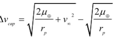
Page 8 of 15 Fig. 5: Representation of all possible orientations of an
orbit as a function of argument of the periapsis . The figure shows two orbital planes, one for the Earth’s orbit and one for the asteroid’s orbit. By continuously changing the argument of the periapsis, all possible orientations of the asteroid orbit in the plane are yielded. The two crosses mark the Earth orbital crossing points which are possible only for four different values of the argument of the periapsis . Two arrows show the argument of the periapsis for one of the four configurations.
As shown by Fig. 5, only 4 specific values of yield a MOID equal to zero (i.e., an intersection between the two orbits). Except if the semilatus rectum
p is equal to 1, in which case there will be only two
values of yielding two simultaneous crossing points. Equation (8) already provided the two possible true anomalies that give the asteroid a distance of 1AU from the Sun. Therefore, for the orbital intersection to occur in the non-ecliptic asteroid case, one of these two angles is required to coincide with the line of nodes, i.e., the straight line where the two orbital planes meet. This yields four different arguments of the periapsis for which the MOID is 0:
0
MOID enc enc enc enc
(24)
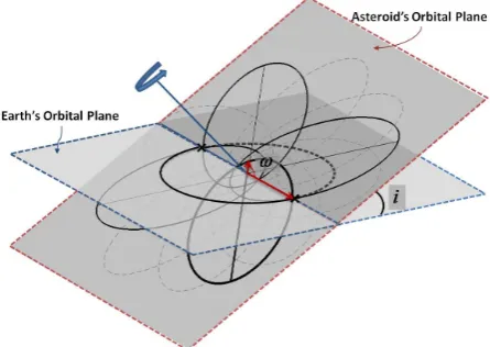
Close to the values of MOID0, the variation of MOID
[image:9.595.74.297.107.265.2]as a function of periapsis argument can be approximated linearly[18, 20]. With the axis shown in Fig. 6, the motion of the Earth and the asteroid can be well described using a linear approximation of the Keplerian velocities of the two objects at the line of nodes. This defines two straight line trajectories, and thus, the minimum distance between these two linear trajectories can be found.
Fig. 6: Set of coordinates used to compute Eq.(25).
The minimum distance can then be written as an explicit function of ∆x (i.e., distance between the centre of the coordinates described in Fig. 6 and the point at which the asteroid crosses the Earth orbital plane), which can also be described as a linear function of the argument of the periapsis . Finally, an expression such as:
0
2
2
min
1
tan sin
MOID MOID
i
(25)
yields an approximate value of the MOID distance. The expression min[|.|] denotes the minimum value of the absolute differences with any of the angles MOID0 and
the tangent of the flight path angle can be calculated as:
22
tan
1
p
e p
(26)
For a complete derivation of a similar formulae, the reader can refer to Opik’s work[18] or alternatively to Bonanno’s work[20]. Note that Eq.(25) is valid only for values of close to any of the values of MOID0 from
Page 9 of 15 Fig. 7: Comparison between the analytical and
numerical approaches to compute MOID.
Capture at MOID point
Now that it has been shown that the analytical approximation of MOID is a reliable way of assessing the distance between two orbits, we can define the maximum MOID at which the capture of an object is possible given a limiting ∆v budget. Eq.(14), in section II.II, defined the required Earth capture manoeuvre
cap v
as a function of the hyperbolic excess velocity v∞
and the pericentre altitude rp. The latter can also be expressed as an explicit function of the hyperbolic velocity v∞and the impulsive manoeuvre:
2
2
2 2
8 cap
p
cap v r
v v
(27)
Since equation (27) refers to non-coplanar asteroids, the hyperbolic velocity v∞ needs to be calculated as:
3 1 2cos
S
v p
a
i
(28)This expression can be derived by noticing that the relative velocity at the encounter for a non-coplanar asteroid can be expressed as:
vrenc,vnenccos i
renc,vnencsin i
. Finally, in order to know the maximum MOID at which a direct capture is possible, the distance rp needs to be corrected by the hyperbolic factor, i.e., factor that accounts for the gravitational attraction of the Earth during the asteroid’s final approach to the Earth. This results on:2
2
MOIDcap p 1
p r
r v
(29)
Note that if the perigee altitude resulting from Eq.(27) is smaller than the radius of the Earth, this would mean that the capture of that particular body is not feasible under that particular ∆v threshold used. In fact, the feasible limit for a fly-by was set to 200km altitude from the surface of the Earth, also to account for the Earth’s atmosphere.
Fraction of capturable asteroids
The previous section provided the means of calculating the MOID at which capture is possible as a
function of vcap. Using the linearly approximated
MOID in Eq.(25), we can see that within a distance ∆ of MOID0 such as:
2
2
1
MOID tan
sin
cap
i
(30)
a direct capture of the asteroid is possible, since the minimum orbital distance is ensured to be smaller than
MOIDcap, and thus, the capture impulse should be
smaller than vcap. One may think then that the total
range at the neighbourhood of MOID0 is 2∆ , and since
there are 4 different MOID0, the total range of at
which capture is possible should be 8∆ . This is
generally correct, but attention must be payed when overlapping of the ranges occurs. If the semilatus rectum p is close to 1, the values enc and - enc are also
close and their ranges ( enc±∆ and - enc±∆ ) may
overlap. A correction is applied in those cases.
The fraction of asteroids with given {a,e,i} that can be captured with a given ∆vbudget is then:
, ,
8
, ,
2
lowMOID
a e i
f a e i
(31)
without the overlap correction. The fraction flowMOID provides the fraction of material with Keplerian elements {a,e,i} that could be captured with a single manoeuvre (≤∆vcap) at the Earth. Capture of asteroid
material by means of only one impulse would simplify considerably the engineering challenges of implementing the two-impulse transfer, described in section II, since this type of transfer requires a spacecraft to be sent to deep-space to perform a change of plane.
Keplerian Feasible Regions
The capturable feasible regions using one-impulse transfers in the {a,e} subspace are the same as in section II.II. The only difference between the feasible volume {a,e,i} of the two-impulse and the one-impulse model lies in the inclination. Since no change of inclination is required, the maximum inclination from which asteroids can be captured is greatly increased. The limit threshold can be computed by realising that v∞ calculated as in Eq.(28) must be equal to v∞ calculated as in Eq.(16), thus:
1 2max
1 1
, , cos 3
2 S
v
i a e v a
p
(32)
where v∞ is calculated as in Eq.(16) with an
200
p
r r km.
0 50 100 150 200 250 300 350 10-3
10-2 10-1 100
Argument of the Periapsis, deg
M
O
ID
, A
U
0 50 100 150 200 250 300 35010
-2
10-1 100 101 102
D
if
fe
r
e
n
c
e
,%
Difference between numerically and analitically calculated MOID
Page 10 of 15 Probability to find an accessible asteroid
Finally, the probability to find an asteroid in an accessible initial orbit (i.e., accessible by using one-impulse transfer) is:
max max max
min min 1
0 , , , ,
imp a e i
lowMOID a e
thr
P
a e i f a e i di de da
v
(33)where P1imp functional dependency with ∆vthr is in the
limits of the integration, which are defined by Eqs.(18), (15), (17) and (32).
III.IV Average accessible mass.
At this point, the probability to find accessible objects (Eqs.(23) and (33)) and the size population model in section II.I can be combined in order to estimate the available material that could be exploited for future space ventures. The accessible material will be mapped as a function of the limiting ∆v budget, and as described in the previous two sections, once a ∆v
threshold has been defined, the probability to find accessible material is computed by integrating Eq.(23) and Eq.(33) for two and one impulse transfers respectively. When the probabilities P2imp and P1imp are
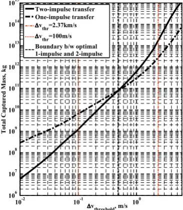
[image:11.595.86.269.445.654.2]known, the average accessible mass of near Earth object material can be calculated by multiplying these probabilities with the total mass of asteroids yielded by Eq.(5) considering objects between 32 km (i.e., largest Near Earth object known today) and 1 meter diameter. Fig. 8 shows the results of accessible asteroid mass as a function of ∆v threshold.
Fig. 8: Average accessible asteroid mass for exploitation of resources as a function of ∆v threshold.
The results in Fig. 8 allow a direct comparison between lunar and asteroid resource exploitation. For a
threshold
v
equal to the Moon’s escape velocity (i.e., 2.37
km/s) the average accessible asteroid material is of the
order of 1.75x10¹³ kg using a two-impulse transfer as
described in this paper. Approximately, 3x10¹²kg of
material could also be captured during Earth fly-by, without having to modify the orbit geometry of these objects. Even if the same vthresholdprovides access to
many orders of magnitude more material at the Moon (i.e., mass of the Moon), the main advantage of asteroid resources with respect lunar resources is that asteroidal material can be exploited at a whole spectrum of ∆v. For example, 6.4x10⁹kg of asteroid resources could still be exploited at a vthresholdof only 100 m/s by using a
serendipitous capture such as the one described by the one-impulse transfer. Lunar material instead requires an energy threshold to overcome the Moon’s gravity well (i.e., a ∆v of 2.37 km/s). On the other hand, the Moon is believed to be a relatively resource-poor body [2], thus asteroid resource exploitation above 2.37 km/s may still be an attractive option.
III.V Phasing maneuvre
Previous sections have assumed that if the orbital intersection exists, then the asteroid would eventually meet the Earth. This statement may be true if the time available to transfer the asteroid is not constrained, but for realistic scenarios this does not occur. Therefore, some analysis on the cost of the manoeuvring necessary to ensure the encounter opportunity must be performed.
For a more realistic transfer scenario, in which the orbital phasing is also considered, an additional impulsive manoeuvre may be necessary in order to provide the correct phasing to the asteroid. This manoeuvre is generally small and must be provided as early as possible, so that the secular effect due to the change in period yields the orbital drift necessary for the asteroid to be at the Earth orbital crossing point at the required time. Hence, if only secular effects are considered[21-22], which is regarded as a good approximation for the level of accuracy intended in this paper, the phasing manoeuvre should correct the
difference in mean anomaly ∆M that exists for the
intended encounter (see Fig. 3). This is expressed as:
e m
M n t t
(34)
where ∆n is the change of mean motion of the asteroid due to the phasing manoeuvre and (te-tm) is the time-span between the manoeuvre (tm) and the encounter (i.e. time at which the Earth is at the crossing point te). The change in mean motion of the asteroid can be defined as:
3 3Sun Sun
n
a
a a
(35)
where a is the change of semi-major axis of the
asteroid due to the impulsive manoeuvre. Using the Gauss planetary equations[23], a can be expressed as:
10-2 10-1 100 106
107 108 109 1010 1011 1012 1013 1014 1015
vthreshold, m/s
T
o
ta
l
C
a
p
tu
re
d
M
a
ss
, k
g
Two-impulse transfer One-impulse transfer
vthr=2.37km/s
Page 11 of 15 0
2
2
t S a v
a v
(36)
where vt is the tangential component of the impulsive manoeuvreand v0 is the orbital velocity at the point at which the impulsive manoeuvre is applied. Eq.(36) seems to indicate that the optimal position for a phasing manoeuvre is the periapsis, since this is the point at
which the orbital velocity v0 is maximum. This is
generally true, except for cases in which the term (te-tm) of equation (34) drives the optimality of the phasing manoeuvre.
Finally, rearranging Eq.(34), (35) and (36), the phasing manoeuvre necessary to drift the asteroid
through ∆M angular position at time te, given a
impulsive manoeuvre at time tm, can be expressed as:
0
1 3
2 2
3
2
S S
t
S
e m
v a
a v M
t t a
(37)
which provides a good estimation of the cost of the phasing manoeuvre to target an Earth encounter.
Considering an Earth-asteroid configuration such as in Fig. 3, an algorithm was implemented that computes the fraction of mean anomalies inside the asteroid orbital path that can be phased with the Earth with a vt smaller than a given threshold. The algorithm requires as an input the ∆M at a given time te at which the Earth is assumed to be at the crossing point from which ∆M is measured. Also a time constraint needs to be specified, which defines the maximum allowed manoeuvre time
[image:12.595.320.513.173.377.2]tmaxm. Then, the algorithm computes the vt necessary to cancel not only the ∆M gap at time te, but also all other possible encounters opportunities, which are defined by the times at which the Earth is at the crossing points during the time-span available. For each possible encounter two manoeuvre times are considered; the first available periapsis passage and tmaxm. This procedure is repeated for many different angular positions ∆M at te, from which then the fraction of the orbit that can be phased under a ∆v limit is calculated.
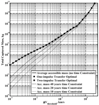
Fig. 9 includes the effect of 40, 20 and 10 years time constraints on the accessibility of asteroid resources. The figure also shows accessibility of asteroid material without considering any time constraint (also shown in Fig. 8), but this time only the results of the optimal transfer strategy are shown for each ∆v threshold. From the results in Fig. 9 it can be concluded that the free phasing assumption during the description of the transfer models is a good approximation for relatively large ∆v thresholds. At low ∆v thresholds some early manoeuvring may be required. Note that a 40-year trajectory may not necessarily be envisaged as a trajectory requiring 40 years to be completed. This only
suggest the necessity to provide early shepherding manoeuvres, allowing asteroids to have the right phasing conditions with Earth. Years later, a short sequence of manoeuvres can be provided to achieve a final capture of the asteroid or its mined material.
Fig. 9: Time constrained and unconstrained accessible mass.
IV. ACCESSIBILITY OF ASTEROIDS One of the important issues not resolved by the results shown in Fig. 8 and Fig. 9 is the number of missions that would require exploiting all or part of the accessible asteroid resources. This issue is of key importance, since if a given resource is spread in a large number of very small objects, gathering all of them may become a cumbersome task, and therefore not economically worthwhile.
In order to estimate the average size of each accessible object, we will assume that each single object has the same probability P (see section III.IV) to be found in the accessible region. Thus, the probability to find k asteroids within a population of n asteroids in a region delimited by the parameter ∆v threshold is well described by the binomial distribution. In this particular case, for which P is a very low probability and n a very large number of asteroids, Poisson distribution (a limiting case of the binomial distribution when n tends to infinity) represents a very good approximation of the statistical behaviour of the problem. Therefore, the probability g(k, ) to find k asteroids when the expected number is can be described by:
,
!k e g k
k
(38)
The expected number , or average number of accessible asteroids, can be calculated as:
10-3 10-2 10-1 100 104
105 106 107 108 109 1010 1011 1012 1013
Vthreshold, km/s
To
ta
l C
a
p
tu
r
ed
M
a
ss
,
k
g
Average accessible mass (no time Constraint) One-impulse Transfer Optimal
[image:12.595.94.291.282.351.2]Page 12 of 15
Dmin
N D
min D Dmax
P (39)
where ∆N is the total number of asteroids with
diameters larger than Dmin and smaller than Dmax
(Eq.(2)) and P the probability to find objects within a given Keplerian region. In the following, ∆N will keep
Dmax fixed to the 32-km diameter, while Dmin may vary
to modify the value of as required. An integration such as:
,NEA n
g k
dk
yields the probability to find at least nNEA asteroids
when the expected value, or average, was . By finding then the value of that yields an accumulative probability of 50%,
, min
50%NEA n
g k
D dk
, (40)we can estimate the median diameter of the smallest
object in the nNEA set. This procedure can also be
repeated with accumulative probabilities of 95% and 5% to obtain the 90% confidence region. The results of this procedure can be seen in the following figure.
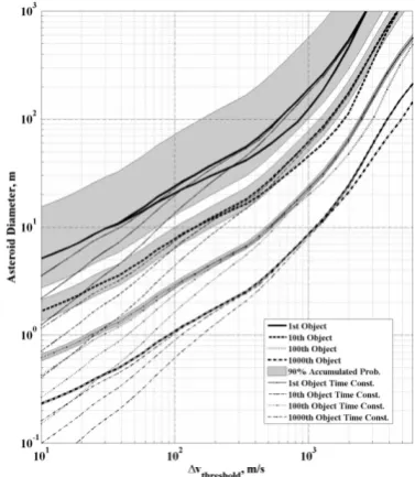
Fig. 10 shows the median diameter of the first, tenth, hundredth and thousandth largest accessible asteroid in the near Earth space, together with the 90% confidence region of each one of these objects. Note that the 90% confidence regions account only for the statistical
uncertainty of finding find k asteroids within a
population of n objects, and that the population is
perfectly described by Eq.(1). The figure also shows the median diameter considering a 2/3 drop in the number of small asteroids as estimated by Harris [24], this is represented by the lower branch in each asteroid set of data. This second population size distribution of asteroids was represented by a three slope power law distribution matching with Eq.(1) at 1-km and 10-m, while providing a 2/3 drop on the accumulative number of asteroids at 100-m. Finally, Fig. 10 also shows the results by considering 40, 20 and 10 years of time constraint in the transfer time, represented as the three departing lines from the main set of data.
The information in the figure can be read as follows: let us set, for example, the ∆v threshold at 100 m/s, the largest accessible object has a 50% probability to be equal to or larger than 24 meters diameter, while we can say with 90% confidence that its size should be between 72 meters and 12 meters. We can also see that when accounting for a population of asteroids as estimated by Harris [24] the median becomes 20 meters instead of 24 meters. Finally, we also see that when time constraints are included and phasing maneuvre are estimated as described in section III.V, the median diameter decays to 23 meters when the constraint is set to 40 years, 20 meters if the constraint is 20 years and 13 meters if the limit is at 10 years (solid-dotted lines). The following
[image:13.595.319.508.184.401.2]set of data in the decreasing ordinate axis is the group referring to the 10th largest object found within the region of feasible capture given by a ∆v threshold of 100 m/s, whose median diameter is at 8 meters diameter. The 100th largest object is foreseen to have a diameter of 3 meters and 1000th largest of 1 meter.
Fig. 10: Expected size of the accessible asteroid.
V. FINAL DISCUSSION
The results shown from Fig. 8 to Fig. 10 indicate the feasibility of future asteroid resource utilisation. One can imagine advantageous scenarios for space utilisation from the results on the expected size of the accessible material (Fig. 10).For example, the exploitation of the largest expected object found within a 100 m/s budget, a 24-m asteroid, could supply from 107kg to 4x10⁷kg of asteroid material, depending on composition and density. If this object was a hydrated carbonaceous asteroids a million litres of water could possibly be extracted (considering an asteroid of density 1300 kg/m3 [15] and 8% [25] of its weight in water). However, if this object was an M-class asteroid (density 5300 kg/m3 [15]), of order thirty thousand tonnes of metal could potentially be extracted and even a tonne of Platinum Group Metals (PGM) (88% of metal assumed and 35ppm of PGM [25]). The latter resource could easily reach a value of fifty million dollars n Earth’s
commodity markets. If the ∆v budget is increased to
1km/s, one 190-m diameter object should be accessible. This corresponds to more than 300 million litres of water or more than 10 million tons of metal and 600 tons of PGMs valued at 30 billion dollars.
Page 13 of 15 propellant. Thus, most likely, this commodity in
particular may represent a very important resource for exploitation in a near future. If water is mined and finally transported to LEO by adding 3.3 km/s to the ∆v
cost estimated here (v thresholdprovided in Fig. 8 to Fig. 10 is the change of velocity required for a weakly bound Earth orbit), the total cost of transportation will still be of order 3 times less that that required to transport the water from the Earth surface. In a scenario such this a 24-m hydrated asteroid could propel a 200 tonne payload from LEO to the surface of the moon. More importantly, the energy invested in transporting this propellant would be a third of that necessary to transport the propellant from the Earth’s surface to LEO. Of course, in order for this scenario to be preferable over the more traditional Earth transport, the cost of mining and transporting the resources back to Earth should be lower than the two-thirds saving on transportation cost. Clearly, this figure improves significantly if the propellant is transported to the Earth-Moon Lagrangian points and used to fuel interplanetary missions [26]. For such a scenario, a mission to Mars would require to be launched only with the propellant to reach the Earth-Moon equilibrium points, which implies launch mass savings of at least a factor of two.
As noted previously, asteroids could be mined and their resources transported to the Earth-Moon system. In fact the transport of material could well benefit from the resources found at the asteroid, and, for example, use water as a propellant found in-situ. However, mining operations may entail a technical complexity, both for manned missions and robotic exploration, that may make the possibility of capturing material directly in Earth orbit a desirable option. The possibility of moving the entire asteroid into an Earth bound orbit would allow much higher mission flexibility for resource extraction and transfer operations. In this kind of scenario, concepts for asteroid deflection technologies could be usefully exploited [6]. Although, each asteroid transfer should be carefully design and optimised, by using some of the technologies envisaged for asteroid deflection some general estimations of spacecraft mass in orbit can be provided. For example, a 10-m asteroid could potentially be found with an estimated capture ∆v
of 30 m/s using a one-impulse type of transfer. Even such a small object could still supply 50 tonnes of water or 600 tonnes of metals and PGMs with a possible market value of one million dollars. An object of this size could be capture during its Earth encounter by providing a collision with a 5-tonne spacecraft at a speed between 4 and 17 km/s, depending on the type of object, and therefore its density and mass. A kinetic impact scenario like this can be easily envisaged considering that the asteroid would be moving at a speed of 11 km/s at the perigee. Even more appealing is the possibility of a ballistic capture of such objects. This
10-m object would be expected to have a relative velocity with the Earth lower than 1km/s, which makes it a suitable candidate for a ballistic capture at the Earth by exploiting three-body dynamics [27].
The analysis and results presented in this paper are intended to provide a qualitative analysis on the feasibility of asteroid exploitation. The results and subsequent discussion have only drawn the ‘big picture’ for future asteroid resource utilisation. The hypothesis from which this work is based have tried to be as conservatives as possible, so that the real accessible mass should be expected to be higher. For example, the transfer models provided a conservative, worst case
scenario for the required ∆v, and so the available
asteroid mass found is then a lower limit. More complex trajectories, such as multiple Earth fly-by, lunar gravity assists or manifold dynamics, would be expected to provide a significant increase in captured mass. However, some hypothesis will require of future work to completely assess their significance. For example, the assumption on the orbital distribution being independent of the asteroid size [8]. Non-gravitational perturbations affect objects of different size differently, which implies that the different asteroid sources may be supplying different asteroid size distributions, since non-gravitational perturbations are the main mechanisms that feed the different asteroid sources. For the same reason, different orbital regions may contain a higher population of a given type of asteroids (i.e., different composition). Despite these possible sources of inaccuracy, the results shown in the paper should still hold their qualitative value.
V. CONCLUSIONS
![Fig. 1: Accumulative size distribution of Near Earth Objects (from Stokes et al. [7])](https://thumb-us.123doks.com/thumbv2/123dok_us/1696213.123007/4.595.74.290.105.278/fig-accumulative-size-distribution-near-earth-objects-stokes.webp)
![Fig. 2: Bottke et al.[8] probability distribution built as](https://thumb-us.123doks.com/thumbv2/123dok_us/1696213.123007/5.595.74.292.425.548/fig-bottke-et-al-probability-distribution-built.webp)