The SIS Epidemic Model with Markovian Switching
A. Gray, D. Greenhalgh, X. Mao, J. Pan Department of Mathematics and Statistics, University of Strathclyde, Glasgow G1 1XH, U.K.
Abstract
Population systems are often subject to environmental noise. Motivated by Takeuchi et al. [36], we will discuss in this paper the effect of telegraph noise on the well-known SIS epidemic model. We establish the explicit solution of the stochastic SIS epidemic model, which is useful in performing computer simulations. We also establish the conditions for extinction and persistence for the stochastic SIS epidemic model and compare these with the corresponding conditions for the deterministic SIS epidemic model. We first prove these results for a two-state Markov chain and then generalise them to a finite state space Markov chain. Computer simulations based on the explicit solution and the Euler–Maruyama scheme are performed to illustrate our theory. We include a more realistic example using appropriate parameter values for the spread ofStreptococcus pneumoniaein children.
Key words: SIS epidemic model, Markov chain, extinction, persistence,Streptococcus pneumoniae.
1
Introduction
Population systems are often subject to environmental noise and there are various types of environmental
noise, e.g. white or colour noise (see e.g. [11, 15, 25, 26, 28, 34, 36]). It is therefore critical to discover whether
the presence of such noise affects population systems significantly.
For example, consider a predator-prey Lotka-Volterra model
˙
x1(t) =x1(t)(a1−b1x2(t)),
˙
x2(t) =x2(t)(−c1+d1x1(t)),
(1.1)
where a1, b1, c1 and d1 are positive numbers. It is well known that the population develops periodically if
there is no influence of environmental noise (see e.g. [14, 35]). However, if the factor of environmental noise is
taken into account, the system will change significantly. Consider a simple colour noise, say telegraph noise.
Telegraph noise can be illustrated as a switching between two or more regimes of environment, which differ by
factors such as nutrition or rainfall (see e.g. [11, 34]). The switching is memoryless and the waiting time for
the next switch has an exponential distribution. We can hence model the regime switching by a finite-state
(1.1) when it is in regime 1, while it obeys another predator-prey Lotka-Volterra model
˙
x1(t) =x1(t)(a2−b2x2(t)),
˙
x2(t) =x2(t)(−c2+d2x1(t))
(1.2)
in regime 2. The switching between these two regimes is governed by a Markov chain r(t) on the state space
S={1,2}. The population system under regime switching can therefore be described by the stochastic model
˙
x1(t) =x1(t)(ar(t)−br(t)x2(t)),
˙
x2(t) =x2(t)(−cr(t)+dr(t)x1(t)).
(1.3)
This system is operated as follows: If r(0) = 1, the system obeys equation (1.1) till timeτ1 when the Markov
chain jumps to state 2 from state 1; the system will then obey equation (1.2) from time τ1 till time τ2 when
the Markov chain jumps to state 1 from state 2. The system will continue to switch as long as the Markov
chain jumps. If r(0) = 2, the system will switch similarly. In other words, equation (1.3) can be regarded
as equations (1.1) and (1.2) combined, switching from one to the other according to the law of the Markov
chain. Equations (1.1) and (1.2) are hence called the subsystems of equation (1.3).
Clearly, equations (1.1) and (1.2) have their unique positive equilibrium states as (p1, q1) = (c1/d1, a1/b1)
and (p2, q2) = (c2/d2, a2/b2), respectively. Recently, Takeuchi et al. [36] revealed a very interesting and
surprising result: If the two equilibrium states of the subsystems are different, then all positive trajectories
of equation (1.3) always exit from any compact set of R2
+ with probability 1; on the other hand, if the two
equilibrium states coincide, then the trajectory either leaves from any compact set of R2+ or converges to
the equilibrium state. In practice, two equilibrium states are usually different, whence Takeuchi et al. [36]
show that equation (1.3) is neither permanent nor dissipative. This is an important result as it reveals the
significant effect of environmental noise on the population system: both subsystems (1.1) and (1.2) develop
periodically, but switching between them makes them become neither permanent nor dissipative.
Markovian environments are also very popular in many other fields of biology. As examples Padilla
and Adolph [32] present a mathematical model for predicting the expected fitness of phenotypically plastic
organisms experiencing a variable environment and discuss the importance of time delays in this model,
and Anderson [1] discusses the optimal exploitation strategies for an animal population in a Markovian
environment. Additionally Peccoud and Ycart [33] propose a Markovian model for the gene induction process,
and Caswell and Cohen [8] discuss the effects of the spectra of the environmental variation in the coexistence
of metapopulations.
Motivated by Takeuchi et al. [36], we will discuss the effect of telegraph noise on the well-known SIS
epidemic model [17, 18]. The SIS epidemic model is one of the simplest epidemic models and is often used in the
literature to model diseases for which there is no immunity. Examples of such diseases include gonorrhea [18],
pneumococcus [21, 23] and tuberculosis. Continuous time Markov chain and stochastic differential equation
SIS epidemic models are discussed by Brauer et al. [6] in their textbook. Ianelli, Milner and Pugliese [20]
deterministic and stochastic SIS epidemic models. Li, Ma and Zhu [22] analyse backward bifurcation in an
SIS epidemic model with vaccination and Van den Driessche and Watmough [37] study backward bifurcation
in an SIS epidemic model with hysteresis. More recently, Andersson and Lindenstrand [3] analyse an open
population stochastic SIS epidemic model where both infectious and susceptible individuals reproduce and die.
Gray et al. [16] establish the stochastic SIS model by parameter perturbation. There are many other examples
of SIS epidemic models in the literature. Also, other two similar models for diseases with permanent immunity
and diseases with a latent period before becoming infectious, the SIR (Susceptible-Infectious-Recovered) and
the SEIR (Susceptible-Exposed-Infectious-Recovered) model respectively are studied by Yang et al. [39] and
stochastic perturbations are introduced in these two models. Liu and Stechlinski [24] analyse the stochastic
SIR model with contact rate being modelled by a switching parameter. Bhattacharyya and Mukhopadhyay
[5] study the SI (Susceptible-Infected) model for prey disease with prey harvesting and predator switching.
Artelejo, Economou and Lopez-Herrero [4] propose some efficient methods to obtain the distribution of the
number of recovered individuals and discuss its relationship with the final epidemic size in the SIS and SIR
stochastic epidemic models.
The classical deterministic SIS epidemic model is described by the following 2-dimensional ODE
dS(t)
dt =µN−βS(t)I(t) +γI(t)−µS(t),
dI(t)
dt =βS(t)I(t)−(µ+γ)I(t),
(1.4)
subject to S(t) +I(t) =N, along with the initial values S(0) = S0 >0 and I(0) = I0 >0, where I(t) and
S(t) are respectively the number of infectious and susceptible individuals at time t in a population of size
N, and µ andγ−1 are the average death rate and the average infectious period respectively. β is the disease
transmission coefficient, so that β = λ/N, where λ is the disease contact rate of an infective individual. λ
is the per day average number of contacts which if made with a susceptible individual would result in the
susceptible individual becoming infected.
It is easy to see thatI(t) obeys the scalar Lotka–Volterra model
dI(t)
dt =I(t)[βN −µ−γ−βI(t)], (1.5)
which has the explicit solution
I(t) =
h
e−(βN−µ−γ)t1
I0 −
β
βN−µ−γ
+βN−βµ−γi−1, ifβN −µ−γ 6= 0,
h
1
I0 +βt
i−1
, ifβN −µ−γ = 0.
(1.6)
Defining the basic reproduction number for the deterministic SIS model
RD0 = βN
µ+γ, (1.7)
we can conclude (see e.g. [35]):
• IfRD
• IfRD
0 >1, limt→∞I(t) = βN−βµ−γ. In this case,I(t) will monotonically decrease or increase to βN−βµ−γ ifI(0)> βN−βµ−γ or< βN−βµ−γ, respectively, whileI(t)≡ βN−βµ−γ ifI(0) = βN−βµ−γ.
Taking into account the environmental noise, the system parameters µ,β and γ may experience abrupt
changes. In the same fashion as in Takeuchi et al. [36], we may model these abrupt changes by a Markov
chain. As a result, the classical SIS model (1.4) evolves to a stochastic SIS model with Markovian switching
of the form
dS(t)
dt =µr(t)N −βr(t)S(t)I(t) +γr(t)I(t)−µr(t)S(t),
dI(t)
dt =βr(t)S(t)I(t)−(µr(t)+γr(t))I(t),
(1.8)
where r(t) is a Markov chain with a finite state space. The main aim of this paper is to discuss the effect of
the noise in the form of Markov switching. We will not only show the explicit solution but will also investigate
the asymptotic properties, including extinction and persistence.
To make our theory more understandable, we will begin with the special case where the Markov chain
has only 2 states, as in Takeuchi et al. [36]. We will then generalise our theory to the general case where the
Markov chain has a finite number of states, M.
2
SIS Model with Markovian Switching
Throughout this paper, unless otherwise specified, we let (Ω,F,{Ft}t≥0,P) be a complete probability space
with a filtration {Ft}t≥0 satisfying the usual conditions (i.e. it is increasing and right continuous while F0
contains all P-null sets). Let r(t), t≥0, be a right-continuous Markov chain on the probability space taking
values in the state space S={1,2} with the generator
Γ =
−ν12 ν12
ν21 −ν21
.
Here ν12 >0 is the transition rate from state 1 to 2, while ν21 >0 is the transition rate from state 2 to 1,
that is
P{r(t+δ) = 2|r(t) = 1}=ν12δ+o(δ) and P{r(t+δ) = 1|r(t) = 2}=ν21δ+o(δ),
where δ > 0. It is well known (see e.g. [2]) that almost every sample path ofr(·) is a right continuous step
function with a finite number of sample jumps in any finite subinterval of R+ := [0,∞). More precisely, there
is a sequence{τk}k≥0 of finite-valued Ft-stopping times such that 0 =τ0< τ1 <· · ·< τk → ∞ almost surely
and
r(t) = ∞
X
k=0
r(τk)I[τk,τk+1)(t), (2.1)
where throughout this paperIAdenotes the indicator function of set A. Moreover, given thatr(τk) = 1, the
random variable τk+1−τk follows the exponential distribution with parameterν12, namely
while given that r(τk) = 2, τk+1−τk follows the exponential distribution with parameterν21, namely
P(τk+1−τk ≥T|r(τk) = 2) =e−ν21T, ∀T ≥0.
The sample paths of the Markov chain can therefore be simulated easily using these exponential distributions
(we will illustrate this in Section 6 below). Furthermore, this Markov chain has a unique stationary distribution
Π = (π1, π2) given by
π1 =
ν21
ν12+ν21
, π2 =
ν12
ν12+ν21
. (2.2)
After recalling these fundamental concepts of the Markov chain, let us return to the stochastic SIS
epidemic model (1.8). We assume that the system parameters βi, µi, γi (i ∈ S) are all positive numbers.
Given that I(t) +S(t) = N, we see that I(t), the number of infectious individuals, obeys the stochastic
Lotka–Volterra model with Markovian switching given by
dI(t)
dt =I(t)[αr(t)−βr(t)I(t)], (2.3)
where
αi :=βiN −µi−γi, i∈S. (2.4)
It is sufficient to study equation (2.3) in order to understand the full dynamics of the stochastic SIS epidemic
model (1.8), hence we will concentrate on this equation only in the remainder of this paper. We will refer to
equations (1.8) or (2.3) in the rest of the paper as ‘the stochastic SIS model’ or ‘the stochastic SIS epidemic
model’, although other stochastic versions of the SIS model exist, e.g. a simple Markovian model describing
only demographic stochasticity. The following theorem shows that this equation has an explicit solution for
any given initial value in (0, N).
Theorem 2.1 For any given initial value I(0) =I0 ∈ (0, N), there is a unique solution I(t) on t ∈ R+ to
equation (2.3) such that
P(I(t)∈(0, N) for all t≥0) = 1.
Moreover, the solution has the explicit form
I(t) =
expRt
0αr(s)ds
1
I0 +
Rt
0exp
Rs
0 αr(u)du
βr(s)ds. (2.5)
Proof. Fix any sample path of the Markov chain. Without loss of generality we may assume that this sample
path has its initial value r(0) = 1, as the proof is the same if r(0) = 2. We first observe from (2.1) that
r(t) = 1 for t∈[τ0, τ1). Hence equation (2.3) becomes
dI(t)
dt =I(t)[α1−β1I(t)]
on t ∈ [τ0, τ1). But this equation has a unique solution on the entire set of t ∈ R+ and the solution will
by continuity, for t=τ1 as well. Obtaining I(τ1) ∈(0, N), we further consider equation (2.3) for t∈[τ1, τ2),
which has the form
dI(t)
dt =I(t)[α2−β2I(t)].
This equation has a unique solution on t≥τ1 and the solution will remain within (0, N). Hence the solution
of equation (2.3), I(t), is uniquely determined ont∈[τ1, τ2) and, by continuity, fort=τ2 as well. Repeating
this procedure, we see that equation (2.3) has a unique solution I(t) on t ∈ R+ and the solution remains
within (0, N) with probability one.
After showingI(t)∈(0, N), we may define
y(t) = 1
I(t), t≥0,
in order to obtain the explicit solution. Compute
dy(t)
dt =−
1
I(t)2
dI(t)
dt
=− 1
I(t)2I(t)(αr(t)−βr(t)I(t))
=βr(t)−
αr(t)
I(t)
=βr(t)−αr(t)y(t).
By the well-known variation-of-constants formula (see e.g. [28, p.96]), we have
y(t) = Φ(t)y(0) +
Z t
0
Φ−1(s)βr(s)ds
,
where Φ(t) =e−R0tαr(s)ds. This yields the desired explicit solution (2.5) immediately. 2
3
The Basic Reproduction Number
Naturally we wish to examine the behaviour of the stochastic SIS epidemic model (2.3) and we may ask
what is the corresponding basic reproduction number RS
0? Recall that the basic reproduction number is the
expected number of secondary cases caused by a single newly-infected case entering the disease-free population
at equilibrium [10].
In our case the disease-free equilibrium (DFE) isS=N, I = 0. The individuals can be divided into two
types, those who arrive when r(t) = 1, and those that arrive when r(t) = 2. Suppose that a newly infected
individual enters the DFE when the Markov chain is in state 1. Then the next events that can happen are
that the individual dies at rate µ1, recovers at rate γ1 or the Markov chain switches at rate ν12. Hence the
expected time until the first event is
1
µ1+γ1+ν12
.
During this time each of theN susceptibles at the DFE is infected at rateβ1. So the total expected number
β1N
µ1+γ1+ν12
. (3.1)
If the first event is either that the infected individual dies or recovers, no more people will be infected
before the first switch. If the first event is that the Markov chain switches the expected number of people
infected before the first switch is given by (3.1). Hence whatever happens the expected number of people
infected before the first switch is given by (3.1).
The expected number of individuals infected between the first and second switches is
ν12
µ1+γ1+ν12
β2N
µ2+γ2+ν21
and between the second and third switches
ν21
µ2+γ2+ν21
ν12
µ1+γ1+ν12
β1N
µ1+γ1+ν12
=p β1N µ1+γ1+ν12
where p= ν12ν21
(µ1+γ1+ν12)(µ2+γ2+ν21)
.
Hence this individual infects in total
m11= β1N
µ1+γ1+ν12
(1 +p+p2+. . . ) = β1N
µ1+γ1+ν12
1 1−p
individuals while the Markov chain is in state 1 and
m12=
ν12
µ1+γ1+ν12
β2N
µ2+γ2+ν21
1 1−p
individuals while the Markov chain is in state 2.
Similarly we can derive the expected number of individuals infected by a single newly infected individual
entering the DFE when the Markov chain is in state 2. We deduce that the next generation matrix giving the
expected number of secondary cases caused by a single newly infected individual entering the DFE is
m11 m12
m21 m22
=
1 1−p
a1 p1a2
p2a1 a2
,
wherea1=
β1N
µ1+γ1+ν12
, a2=
β2N
µ2+γ2+ν21
, p1 =
ν12
µ1+γ1+ν12
and
p2 =
ν21
µ2+γ2+ν21
.
The basic reproduction number for the stochastic epidemic model is the largest eigenvalue of this matrix
RS0 = a1+a2+
p
(a1+a2)2−4a1a2(1−p)
2(1−p) . (3.2)
4
Extinction
In the study of the SIS epidemic model, extinction is one of the important issues. In this section we will discuss
this issue. Recall that for the deterministic SIS epidemic model (1.5), the basic reproduction numberRD
0 was
also the threshold between disease extinction and persistence, with extinction forRD
0 ≤1 and persistence for
RD
0 >1. In the stochastic model, there are different types of extinction and persistence, for example almost
sure extinction, extinction in mean square and extinction in probability. In the rest of the paper we examine
a threshold
T0S = π1β1N +π2β2N
π1(µ1+γ1) +π2(µ2+γ2)
(4.1)
for almost sure extinction or persistence of our stochastic epidemic model. However this threshold is different
to RS
0 which might be more relevant to other types of extinction or persistence.
We will see later that the stochastic SIS model (2.3) will become extinct (meaning that limt→∞I(t) = 0)
with probability one ifTS
0 <1. Before we state this result, let us state a proposition which gives an equivalent
condition for TS
0 < 1 in terms of the system parameters αi and the stationary distribution of the Markov
chain.
Proposition 4.1 We have the following alternative condition on the value of TS 0:
• TS
0 <1 if and only if π1α1+π2α2 <0;
• TS
0 = 1 if and only if π1α1+π2α2 = 0;
• TS
0 >1 if and only if π1α1+π2α2 >0.
The proof of this proposition is straightforward, so is omitted. We can now state our theory on extinction.
Theorem 4.2 If TS
0 < 1, then, for any given initial value I0 ∈ (0, N), the solution of the stochastic SIS epidemic model (2.3) obeys
lim sup
t→∞
1
t log(I(t))≤α1π1+α2π2 a.s. (4.2)
By Proposition 4.1, we hence conclude that I(t)tends to zero exponentially almost surely. In other words, the
disease dies out with probability one.
Proof. It is easy to see that
dlog(I(t))
dt =αr(t)−βr(t)I(t). (4.3)
This implies that, for any t >0,
log(I(t))
t ≤
log(I(0))
t +
1
t
Z t
0
sinceβr(t)>0 andI(t)∈(0, N). Letting t→ ∞ we hence obtain
lim sup
t→∞
1
tlog(I(t))≤lim supt→∞ 1
t
Z t
0
αr(s)ds.
However, by the ergodic theory of the Markov chain (see e.g. [2]) we have
lim
t→∞
1
t
Z t
0
αr(s)ds=α1π1+α2π2 a.s.
We therefore must have
lim sup
t→∞
1
t log(I(t))≤α1π1+α2π2 a.s.,
as required. 2
Let us now make a few comments. First of all, let us recall that the stochastic SIS model (2.3) can be
regarded as the result of the following two subsystems
dI(t)
dt =I(t)[α1−β1I(t)] (4.4)
and
dI(t)
dt =I(t)[α2−β2I(t)], (4.5)
switching from one to the other according to the law of the Markov chain. If both α1 <0 and α2 <0, then
the corresponding RD
0 values for both subsystems (4.4) and (4.5) are less than 1, whence both subsystems
become extinct. In this case,TS
0 for the stochastic SIS model (2.3) is less than 1, hence it will become extinct,
and of course this is not surprising. However, if only one ofα1 and α2 is negative, sayα1 <0 andα2 >0, for
example, one subsystem (4.4) becomes extinct but the other (4.5) is persistent. However, if the rate of the
Markov chain switching from state 2 to 1 is relatively faster than that from 1 to 2, so that α1π1+α2π2 <0,
then the overall system (2.3) will become extinct. This reveals the important role of the Markov chain in the
extinction.
We next recall that in the deterministic SIS model (1.5) the disease will always go extinct even ifRD
0 = 1.
The reader may ask what happens to the stochastic SIS model (2.3) if the correspondingTS
0 = 1? Although
we have a strong feeling that the disease will always become extinct, we have not been able to prove it so far.
In Section 6.3 we show some simulations to illustrate this case.
5
Persistence
Let us now turn to the case whenTS
0 >1. The following theorem shows that the disease will be persistent in
this case, meaning that limt→∞I(t)>0.
Theorem 5.1 If TS
0 > 1, then, for any given initial value I0 ∈ (0, N), the solution of the stochastic SIS model (2.3) has the properties that
lim inf
t→∞ I(t)≤
π1α1+π2α2
π1β1+π2β2
and
lim sup
t→∞
I(t)≥ π1α1+π2α2
π1β1+π2β2
a.s. (5.2)
In other words, the disease will reach the neighbourhood of the level π1α1+π2α2
π1β1+π2β2 infinitely many times with
probability one.
Proof. Let us first prove assertion (5.1). If this were not true, then we can find an ε >0 sufficiently small
forP(Ω1)>0 where
Ω1 =
ω ∈Ω : lim inf
t→∞ I(t)>
π1α1+π2α2
π1β1+π2β2
+ε
. (5.3)
On the other hand, by the ergodic theory of the Markov chain, we have thatP(Ω2) = 1, where for anyω∈Ω2,
lim t→∞ 1 t Z t 0
αr(s)−βr(s)
hπ
1α1+π2α2
π1β1+π2β2
+εids
= π1
α1−β1
hπ1α1+π2α2
π1β1+π2β2
+εi+π2
α2−β2
hπ1α1+π2α2
π1β1+π2β2
+εi
= −(π1β1+π2β2)ε. (5.4)
Now consider any ω∈Ω1∩Ω2. Then there is a positive numberT =T(ω) such that
I(t)≥ π1α1+π2α2
π1β1+π2β2
+ε ∀t≥T.
It then follows from (4.3) that
log(I(t))≤log(I0) +
Z T
0
(αr(s)−βr(s)I(s))ds+
Z t
T
αr(s)−βr(s)
hπ
1α1+π2α2
π1β1+π2β2
+εids
for all t≥T. Dividing both sides by tand then letting t→ ∞, we obtain that
lim sup
t→∞
1
t log(I(t))≤ −(π1β1+π2β2)ε,
where (5.4) has been used. This implies that
lim
t→∞I(t) = 0.
But this contradicts (5.3). The required assertion (5.1) must therefore hold.
The procedure to prove assertion (5.2) is very similar. In fact if (5.2) were not true, we can then find an
ε >0 sufficiently small forP(Ω3)>0, where
Ω3 =
ω∈Ω : lim sup
t→∞
I(t)< π1α1+π2α2 π1β1+π2β2 −
ε
. (5.5)
By the ergodic theory we also have thatP(Ω4) = 1, where for anyω ∈Ω4,
lim t→∞ 1 t Z t 0
αr(s)−βr(s)
hπ1α1+π2α2
π1β1+π2β2 −
εids
= π1
α1−β1
hπ1α1+π2α2
π1β1+π2β2
−εi+π2
α2−β2
hπ1α1+π2α2
π1β1+π2β2
−εi
If we consider anyω ∈Ω3∩Ω4, there is a positive numberT =T(ω) such that
I(t)≤ π1α1+π2α2
π1β1+π2β2 −
ε ∀t≥T.
From (4.3) we have that
log(I(t))≥log(I0) +
Z T
0
(αr(s)−βr(s)I(s))ds+
Z t
T
αr(s)−βr(s)
hπ
1α1+π2α2
π1β1+π2β2 −
εids
for all t≥T. Dividing both sides by tand then letting t→ ∞ while using (5.6) as well, we obtain that
lim inf
t→∞
1
t log(I(t))≥(π1β1+π2β2)ε.
This implies that
lim
t→∞I(t)→ ∞,
which contradicts (5.5). Therefore assertion (5.2) must hold.2
To reveal more properties of the stochastic SIS model, we observe from Proposition 4.1 that TS
0 > 1 is
equivalent to the condition that π1α1 +π2α2 > 0. This may be divided into two cases: (a) both α1 and
α2 are positive; and (b) only one of α1 and α2 is positive. Without loss of generality, we may assume that
0 < α1/β1 = α2/β2 or 0 < α1/β1 < α2/β2 in Case (a), while α1/β1 ≤ 0 < α2/β2 in Case (b). So there
are three different cases to be considered under condition TS
0 >1. Let us present a lemma in order to show
another new result.
Lemma 5.2 The following statements hold with probability one:
(i) If0< α1/β1 =α2/β2, then I(t) =α1/β1 for all t >0 when I0=α1/β1.
(ii) If0< α1/β1 < α2/β2, then I(t)∈(α1/β1, α2/β2) for allt >0 whenever I0∈(α1/β1, α2/β2).
(iii) Ifα1/β1 ≤0< α2/β2, then I(t)∈(0, α2/β2) for allt >0 whenever I0∈(0, α2/β2).
Proof. Case (i) is obvious. To prove Case (ii), we may assume, without loss of generality, that r(0) = 1.
Recalling (2.1) and the properties of the deterministic SIS model (1.5) which we stated in Section 1, we
see that I(t) will monotonically decrease during the time interval [τ0, τ1] but never reach α1/β1, whence
I(t) ∈ (α1/β1, α2/β2). At time τ1, the Markov chain switches to state 2 and will not jump to state 1 until
time τ2. During this time interval [τ1, τ2], I(t) will monotonically increase but never reach α2/β2, whence
I(t) ∈ (α1/β1, α2/β2) again. Repeating this argument, we see that I(t) will remain within (α1/β1, α2/β2)
forever. Similarly, we can show Case (iii). 2
In the following study we will use the Markov property of the solutions (see e.g. [27, 29]). For this purpose,
let us denote byPI0,r0 the conditional probability measure generated by the pair of processes (I(t), r(t)) given
the initial condition (I(0), r(0)) = (I0, r0)∈(0, N)×S.
Theorem 5.3 Assume that TS
(i) If0< α1/β1 =α2/β2, then limt→∞I(t) =α1/β1.
(ii) If0< α1/β1 < α2/β2, then
α1
β1 ≤
lim inf
t→∞ I(t)≤lim supt→∞ I(t)≤
α2
β2
.
(iii) Ifα1/β1 ≤0< α2/β2, then
0≤lim inf
t→∞ I(t)≤lim supt→∞ I(t)≤
α2
β2
.
Proof. Case (i). If I0 =α1/β1, then I(t) =α1/β1 for all t≥0, whence the assertion holds. If I0 < α1/β1,
it is easy to see that I(t) increases monotonically on t ≥ 0, hence limt→∞I(t) exists. By Theorem 5.1, we therefore have
lim
t→∞I(t) =
π1α1+π2α2
π1β1+π2β2
a.s.
But, given α1/β1 =α2/β2, we compute
π1α1+π2α2
π1β1+π2β2
= π1α1+π2α1β2/β1
π1β1+π2β2
= α1
β1
.
We therefore have limt→∞I(t) =α1/β1 a.s. Similarly, we can show this for I0 > α1/β1.
Case (ii). IfI0∈(α1/β1, α2/β2), then the assertion follows from Lemma 5.2 directly. Let us now assume
that I0 ≥α2/β2. Given 0< α1/β1 < α2/β2, it is easy to show that
α1
β1
< π1α1+π2α2 π1β1+π2β2
< α2 β2
.
Consider a number
κ∈π1α1+π2α2
π1β1+π2β2
, α2 β2
,
and define the stopping time
ρκ= inf{t≥0 :I(t)≤κ},
where throughout this paper we set inf∅=∞ (in which ∅denotes the empty set as usual). By Theorem 5.1
we have
P(ρk<∞) = 1,
while by the continuity of I(t) we have I(ρκ) =κ. Set
¯
Ω =nα1/β1 ≤lim inf
t→∞ I(t)≤lim supt→∞ I(t)≤α2/β2
o
and denote its indicator function by I¯
Ω. By the strong Markov property, we compute
P( ¯Ω) =E(IΩ¯) = E(E(IΩ¯|Fρ
κ)) =
E(E(IΩ¯|I(ρκ), r(ρκ))) =E(PI(ρ
κ),r(ρκ)( ¯Ω)) =E(Pκ,r(ρκ)( ¯Ω)).
But, by Lemma 5.2, Pκ,r(ρ
κ)( ¯Ω) = 1 and hence we have P( ¯Ω) = 1 as required. Similarly, we can show that
Case (iii). It is obvious that 0≤lim inft→0I(t), while the assertion that lim inft→0I(t) ≤α2/β2 can be
proved in the same way as Case (ii) was proved. The proof is therefore complete. 2
Under the condition TS
0 > 1, the theorem above shows precisely that I(t) will tend to α1/β1 with
probability one if α1/β1 =α2/β2. However, it is quite rare to haveα1/β1 =α2/β2 in practice. It is therefore
more useful to study the case when, say, α1/β1 < α2/β2 in a bit more detail. In the proof above, we have in
fact shown a slightly stronger result than Theorem 5.3 states, namely we have shown that
P(I(t)∈(0∨(α1/β1), α2/β2) for allt≥ρκ) = 1, (5.7)
where we use the notation a∨b= max(a, b). It would be interesting to find out howI(t) will vary within the
interval (0∨(α1/β1), α2/β2) in the long term. The following theorem shows thatI(t) can take any value up
to the boundaries of the interval infinitely many times (though never reach them) with positive probability.
Theorem 5.4 Assume that TS
0 >1 and 0< αβ11 <
α2
β2, and let I0 ∈(0, N) be arbitrary. Then for anyε > 0,
sufficiently small for
α1
β1
+ε < π1α1+π2α2 π1β1+π2β2
< α2 β2 −
ε,
the solution of the stochastic SIS epidemic model (2.3) has the properties that
Plim inf
t→∞ I(t)<
α1
β1
+ε≥e−ν12T1(ε), (5.8)
and
P
lim sup
t→∞
I(t)> α2 β2 −
ε≥e−ν21T2(ε), (5.9)
where T1(ε)>0 and T2(ε)>0 are defined by
T1(ε) =
1
α1
logβ1
α1 −
β2
α2
+ logα1
β1
+ε−logεβ1
α1
(5.10)
and
T2(ε) =
1
α2
logβ1
α1 −
β2
α2
+ logα2
β2 −
ε−logεβ2
α2
. (5.11)
Proof. LetT >0 be arbitrary. Define the stopping time
σ1 = inf{t≥T :I(t)∈(α1/β1+ε, α2/β2−ε)}.
By Theorem 5.1, we have P(σ1 <∞) = 1, while we see from the proof of Theorem 5.3 that
P(I(t)∈(α1/β1, α2/β2) for all t≥σ1) = 1. (5.12)
To prove assertion (5.8), we define another stopping time
σ2= inf{t≥σ1:r(t) = 1}.
Clearly, P(σ2 < ∞) = 1 and by the right-continuity of the Markov chain, r(σ2) = 1. By the memoryless
property of an exponential distribution, the probability that the Markov chain will not jump to state 2 before
σ2+T1(ε) is
where Ω1 = {r(σ2 +t) = 1 for allt ∈ [0, T1(ε)]}. Now, consider any ω ∈ Ω1 and consider I(t) on t ∈
[σ2, σ2+T1(ε)]. Note that it obeys the differential equation
dI(t)
dt =I(t)(α1−β1I(t)),
with initial value I(σ2)∈(α1/β1, α2/β2). By the explicit solution of this equation (see Section 1), we have
I(σ2+T1(ε)) =
h
e−α1T1(ε) 1
I(σ2) −
β1
α1
+ β1
α1
i−1
.
On the other hand, by (5.10), we have
h
e−α1T1(ε)
β
2
α2 −
β1
α1
+ β1
α1
i−1
= α1
β1
+ε.
Since I(σ2)< α2/β2, we must therefore have
I(σ2+T1(ε))<
α1
β1
+ε.
Consequently
P inf
T≤t<∞I(t)<
α1
β1
+ε≥P(Ω1) =e−ν12T1(ε). (5.14)
Noting that
lim inf
t→∞ I(t)<
α1
β1
+ε= \
0<T <∞
inf
T≤t<∞I(t)<
α1
β1
+ε,
we can let T → ∞ in (5.14) to obtain assertion (5.8). Similarly, we can prove the other assertion (5.9). 2
Theorem 5.5 Assume thatTS
0 >1(namely π1α1+π2α2 >0) and βα11 ≤0< αβ22. LetI0∈(0, N) be arbitrary. Then for any ε >0, sufficiently small for
ε < π1α1+π2α2 π1β1+π2β2
< α2 β2
−ε,
the solution of the stochastic SIS model (2.3) has the properties that
Plim inf
t→∞ I(t)< ε
≥e−ν12T3(ε), (5.15)
and
P
lim sup
t→∞
I(t)> α2 β2 −
ε≥e−ν21T4(ε), (5.16)
where T3(ε)>0 and T4(ε)>0 are defined by
T3(ε) =
1
α1
logβ2
α2 −
β1
α1
+ logεα1 β1
−logα1
β1 −
ε (5.17)
and
T4(ε) =
1
α2
log2
ε− β2
α2
+ logα2
β2
−ε−logεβ2
α2
Proof. LetT >0 be arbitrary. Define the stopping time
σ3 = inf{t≥T :I(t)∈(ε, α2/β2−ε)}.
By Theorem 5.1, we have P(σ3 <∞) = 1, while we see from the proof of Theorem 5.3 that
P(I(t)∈(0, α2/β2) for all t≥σ3) = 1. (5.19)
To prove assertion (5.15), we define another stopping time
σ4= inf{t≥σ3:r(t) = 1}.
Clearly, P(σ4 < ∞) = 1 and by the right-continuity of the Markov chain, r(σ4) = 1. By the memoryless
property of an exponential distribution, the probability that the Markov chain will not jump to state 2 before
σ4+T3(ε) is
P(Ω2) =e−ν12T3(ε), (5.20)
where Ω2 = {r(σ4 +t) = 1 for allt ∈ [0, T3(ε)]}. Now, consider any ω ∈ Ω2 and consider I(t) on t ∈
[σ4, σ4+T3(ε)]. Note that it obeys the differential equation
dI(t)
dt =I(t)(α1−β1I(t)),
with initial value I(σ4)∈(0, α2/β2). By the explicit solution of this equation (see Section 1), we have
I(σ4+T3(ε)) =
h
e−α1T3(ε) 1
I(σ4)
−β1
α1
+ β1
α1
i−1
.
On the other hand, by (5.17), we have
h
e−α1T3(ε)
β
2
α2 −
β1
α1
+β1
α1
i−1
=ε.
Since I(σ4)< α2/β2, we must therefore have
I(σ4+T1(ε))< ε.
Consequently
P
inf
T≤t<∞I(t)< ε
≥P(Ω2) =e−ν12T3(ε). (5.21)
Noting that
lim inf
t→∞ I(t)< ε
= \
0<T <∞
inf
T≤t<∞I(t)< ε
,
we can let T → ∞ in (5.21) to obtain assertion (5.15).
To prove the other assertion (5.16) we define the stopping time
σ5 = inf{t≥T :r(t) = 2},
where T >0 is arbitrary. Clearly P(σ5<∞) = 1. We define another stopping time
σ6 = inf
n
t≥σ5:r(t) = 2, I(t)≥
1 2
π
1α1+π2α2
π1β1+π2β2
o
Suppose thatI(t)< 12π1α1+π2α2
π1β1+π2β2
whent=σ5,I(t) will eventually increase across this level by Theorem 5.1.
Note that I(t) increases monotonically whenr(t) = 2 whilst it decreases monotonically whenr(t) = 1. Ifr(t)
switches back to state 1 beforeI(t) increases over this level and starts decreasing, since the lim supt→∞I(t)≥
π1α1+π2α2
π1β1+π2β2, I(t) will increase across this level later on i.e. r(t) = 2 when I(t)=
1 2
π1α1+π2α2
π1β1+π2β2
. Therefore we
have P(σ6 < ∞) = 1. And by the right-continuity of the Markov chain, r(σ6) = 2. By the memoryless
property of an exponential distribution, the probability that the Markov chain will not jump to state 1 before
σ6+T4(ε) is
P(Ω3) =e−ν21T4(ε), (5.22)
where Ω3 = {r(σ6 +t) = 2 for allt ∈ [0, T4(ε)]}. Now, consider any ω ∈ Ω3 and consider I(t) on t ∈
[σ6, σ6+T4(ε)]. Note that it obeys the differential equation
dI(t)
dt =I(t)(α2−β2I(t)),
with initial value I(σ6) ≥ 12
π1α1+π2α2
π1β1+π2β2
> 2ε. By the explicit solution of this equation (see Section 1), we
have
I(σ6+T4(ε)) =
h
e−α2T4(ε) 1
I(σ6) −
β2
α2
+ β2
α2
i−1
.
On the other hand, by (5.18), we have
h
e−α2T4(ε)2
ε− β2
α2
+ β2
α2
i−1
= α2
β2 −
ε.
Since I(σ6)> ε2, we must therefore have
I(σ6+T4(ε))> α2
β2
−ε.
Consequently
P sup
T≤t<∞
I(t)> α2 β2 −
ε≥P(Ω3) =e−ν21T4(ε). (5.23)
Noting that
lim sup
t→∞
I(t)> α2 β2 −
ε= \
0<T <∞
sup
T≤t<∞
I(t)> α2 β2 −
ε,
we can let T → ∞ in (5.23) to obtain assertion (5.16). 2
Define
RD01= β1N
µ1+γ1
andRD02= β2N
µ2+γ2
.
Note that ifαj >0 then R0Dj >1 for j= 1,2 and
αj
βj
=N
1− 1
RD 0j
is the endemic level of disease after a long time in the SIS model (1.4) with β = βj, µ = µj and γ = γj.
the first model the disease prevalence eventually approaches 0∨(α1/β1) and in the second model the disease
prevalence eventually approachesα2/β2. These are the two levels between which the disease oscillates in the
Markov chain switching model.
6
Simulations
In this section we shall assume that all parameters are given in appropriate units.
6.1 Extinction case
Example 6.1.1 Assume that the system parameters are given by
µ1 = 0.45, µ2 = 0.05, γ1 = 0.35, γ2 = 0.15, β1 = 0.001, β2 = 0.004, N = 100,
ν12= 0.6, and ν21= 0.9.
So α1 =−0.7,α2 = 0.2,π1= 0.6, andπ2= 0.4 (see Section 2 for definitions).
Noting that
α1π1+α2π2=−0.34,
we can therefore conclude, by Theorem 4.2, that for any given initial valueI(0) =I0 ∈(0, N), the solution of
(2.3) obeys
lim sup
t→∞
1
tlog(I(t))≤ −0.34<0 a.s.
That is, I(t) will tend to zero exponentially with probability one.
The computer simulation in Figure 1(a) supports this result clearly, illustrating extinction of the disease.
Furthermore, α1 < 0 while α2 > 0 in this case, which means that one subsystem dies out while the other
subsystem is persistent. Figure 1(a) shows some decreasing then increasing behaviour early on, but the general
trend tends to zero, illustrating extinction for the system as a whole. The Euler–Maruyama (EM) method
[28, 29] is also applied to approximate the solution I(t). The two lines are very close to each other, showing
that the EM method gives a very good approximation to the true solution in this case.
Example 6.1.2 Assume that the system parameters are given by
µ1 = 0.45, µ2 = 0.05, γ1 = 0.35, γ2 = 0.15, β1 = 0.006, β2 = 0.0015, N = 100,
ν12= 0.6, and ν21= 0.9.
So α1 =−0.2,α2 =−0.05,π1 = 0.6, andπ2 = 0.4 (see Section 2 for definitions).
Noting that
α1π1+α2π2=−0.14,
we can therefore conclude, by Theorem 4.2, that for any given initial valueI(0) =I0 ∈(0, N), the solution of
(2.3) obeys
lim sup
t→∞
1
0 10 20 30 40 50
0
10
20
30
40
50
60
(a)
t
I(t)
0 10 20 30 40 50
1.0
1.2
1.4
1.6
1.8
2.0
t
r(t)
0 10 20 30 40 50
0
10
20
30
40
50
60
(b)
t
I(t)
0 10 20 30 40 50
1.0
1.2
1.4
1.6
1.8
2.0
t
[image:18.612.91.475.29.366.2]r(t)
Figure 1: Computer simulation ofI(t) and its corresponding Markov chainr(t), using the parameter values in
Example 6.1.1 for (a) and in Example 6.1.2 for (b),I(0) = 60 for both cases, and the exponential distribution
for the switching times ofr(t), withr(0) = 1. The black line is forI(t) using formula (2.5) and the red line is
for the EM method. (The two lines are very close to each other, so we hardly see the black line in the plot.)
That is, I(t) will tend to zero exponentially with probability one. The computer simulation in Figure 1(b)
supports this result clearly, illustrating extinction of the disease. Both α1 and α2 are less than zero in this
case, which means that both subsystems die out. Figure 1(b) shows a trend of decreasing all the time but at
different speeds, which reveals that property. As before, the EM method gives a good approximation in this
case as well.
6.2 Persistence case
Example 6.2.1 Assume that the system parameters are given by
µ1 = 0.45, µ2 = 0.05, γ1 = 0.35, γ2 = 0.15, β1 = 0.01, β2 = 0.012, N = 100,
ν12= 0.6, and ν21= 0.9.
Noting that
α1π1+α2π2 = 0.52,
we can therefore conclude, by Theorem 5.3, that for any given initial valueI(0) =I0 ∈(0, N), the solution of
(2.3) obeys
α1
β1
= 20≤lim inf
t→∞ I(t)≤lim supt→∞ I(t)≤83.33 =
α2
β2
.
That is,I(t) will eventually enter the region (20, 83.33) if I(0) is not in this region, and will be attracted in
this region once it has entered. Also, by Theorem 5.4, I(t) can take any value up to the boundaries of (20,
83.33) but never reach them.
The computer simulations in Figure 2(a), (b) and (c), using different initial values I(0), support these
results clearly. As before, the EM method gives a good approximation of the true solution.
0 10 20 30 40 50
20
40
60
80
(a)
t
I(t)
0 10 20 30 40 50
1.0
1.4
1.8
t
r(t)
0 10 20 30 40 50
20
40
60
80
(b)
t
I(t)
0 10 20 30 40 50
1.0
1.4
1.8
t
r(t)
0 10 20 30 40 50
20
40
60
80
(c)
t
I(t)
0 10 20 30 40 50
1.0
1.4
1.8
t
[image:19.612.90.479.238.584.2]r(t)
Figure 2: Computer simulation ofI(t) and its corresponding Markov chainr(t), using the parameter values in
Example 6.2.1, withI(0) = 15 for (a),I(0) = 60 for (b) andI(0) = 90 for (c), and the exponential distribution
for the switching times of r(t), withr(0) = 1. The black line is for I(t) using formula (2.5) and the red line
for the EM method. (The two lines are very close to each other, so we hardly see the black line in the plot.)
The horizontal lines in the plot of I(t) indicate levels α1
β1 and
α2
Example 6.2.2 Assume that the system parameters are given by
µ1= 0.45, µ2 = 0.05, γ1 = 0.35, γ2 = 0.15, β1 = 0.004, β2 = 0.012, N = 100,
ν12= 0.6, and ν21= 0.9.
So α1 =−0.4,α2 = 1,π1 = 0.6, andπ2= 0.4 .
Noting that
α1π1+α2π2 = 0.16,
we can therefore conclude, by Theorem 5.3, that for any given initial valueI(0) =I0 ∈(0, N), the solution of
(2.3) obeys
0≤lim inf
t→∞ I(t)≤lim supt→∞ I(t)≤83.33 =
α2
β2
.
That is, I(t) will eventually enter the region (0, 83.33) if I(0) is not in this region, and will be attracted in
this region once it has entered. Also, by Theorem 5.5, I(t) can take any value up to the boundaries of (0,
83.33) but never reach them.
The computer simulations in Figure 3 support this result clearly.
0 10 20 30 40 50
0
20
40
60
80
t
I(t)
0 10 20 30 40 50
1.0
1.2
1.4
1.6
1.8
2.0
t
[image:20.612.89.477.338.486.2]r(t)
Figure 3: Computer simulation of I(t) using the parameter values in Example 6.2.2 and its corresponding
Markov chain r(t), using formula (2.5) (black line) and the EM method (red line) for I(t), with I(0) = 60,
and the exponential distribution for the switching times ofr(t), with r(0) = 1. (The two lines are very close
to each other, so we hardly see the black line in the plot.) The horizontal lines in the plot of I(t) indicate the
levels 0 and α2
β2.
6.3 TS
0 =1 Case
Example 6.3.1 Assume that the system parameters are given by
µ1 = 0.45, µ2 = 0.05, γ1 = 0.35, γ2 = 0.15, β1 = 0.006, β2 = 0.005, N = 100,
So α1 =−0.2,α2 = 0.3,π1= 0.6, andπ2= 0.4.
Note that
α1π1+α2π2= 0
in this case, which is equivalent to TS
0 = 1. As mentioned in Section 4, we have not been able to prove the
behaviour of I(t) in this case. However, the simulation results in Figure 4 confirm our suspicion that the
disease will always become extinct.
0 500 1000 1500 2000 2500 3000
0
20
40
60
t
[image:21.612.90.472.169.322.2]I(t)
Figure 4: Computer simulation of I(t) using the parameter values in Example 6.3.1, using formula (2.5) for
I(t), with I(0) = 60, and the exponential distribution for the switching times of r(t), with r(0) = 1.
7
Generalisation
We have discussed the simplest case where the Markov chain has only two states, in the previous sections.
Now we are going to generalise the results to the case where the Markov chain r(t) has finite state space
S={1,2, ..., M}. The generator forr(t) is defined as
Γ = (νij)M×M,
where νii=−P1≤j≤M,j6=iνij,and νij >0 (i6=j) is the transition rate from state ito j, that is
P{r(t+δ) =j|r(t) =i}=νijδ+o(δ),
where δ > 0. As before, there is a sequence {τk}k≥0 of finite-valued Ft-stopping times such that 0 = τ0 <
τ1 <· · ·< τk → ∞almost surely and
r(t) = ∞
X
k=0
r(τk)I[τk,τk+1)(t).
Moreover, given that r(τk) = i, the random variable τk+1 −τk follows the exponential distribution with
parameter −νii, namely
P(τk+1=j|τk=i) = νij
−νii
Furthermore, the unique stationary distribution of this Markov chain Π = (π1, π2, ..., πM) satisfies
ΠΓ = 0
PM
i=1πi= 1.
Following a similar procedure we still can show that for any given initial valueI(0) =I0 ∈(0, N), there
is a unique solutionI(t) on t∈R+ to equation (2.3) such that
P(I(t)∈(0, N) for all t≥0) = 1,
and the solution still has the form (2.5).
In the general finite state space Markov chain case it is possible to derive an explicit expression for the
basic reproduction numberRS0 in the stochastic Markov switching model analogous to (3.2) expressed as the
largest eigenvalue of a positive matrix. We defineTS
0 for the general case as
T0S=
PM
k=1πkβkN
PM
k=1πk(µk+γk)
.
Similarly to Proposition 4.1, we have the following alternative conditions on the value of TS 0 :
Proposition 7.1 We have the following alternative condition on the value of TS 0:
• TS
0 <1 if and only if
PM
k=1πkαk <0;
• T0S = 1 if and only if PM
k=1πkαk = 0;
• TS
0 >1 if and only if
PM
k=1πkαk >0.
IfTS
0 <1, similarly to Theorem 4.2, we can show:
Theorem 7.2 For any given initial value I0 ∈(0, N), the solution of the stochastic SIS model (2.3) obeys
lim sup
t→∞
1
tlog(I(t))≤
M X
k=1
πkαk a.s.
By the more general condition stated above, we hence conclude that I(t) tends to zero exponentially almost
surely. This means that the disease dies out with probability one.
For the case thatTS
0 >1, Theorem 5.1 can be generalised as follows:
Theorem 7.3 If T0S > 1, for any given initial value I0 ∈ (0, N), the solution of the stochastic SIS model
(2.3) has the properties that
lim inf
t→∞ I(t)≤
PM
k=1πkαk
PM
k=1πkβk
a.s.
and
lim sup
t→∞
I(t)≥
PM
k=1πkαk
PM
k=1πkβk
a.s.,
which means the disease will reach the neighbourhood of the level PM
k=1πkαk
PM
k=1πkβk infinitely many times with
Lemma 5.2 can be generalised as follows:
Lemma 7.4 Without loss of generality we assume that α1/β1 ≤ α2/β2 ≤ ... ≤ αM/βM and the following
statements hold with probability one:
(i) If0< α1/β1 =α2/β2 =...=αM/βM, then I(t) =α1/β1 for all t >0 when I0 =α1/β1.
(ii) If 0 < α1/β1 ≤ α2/β2 ≤ ... ≤ αM/βM, then I(t) ∈ (α1/β1, αM/βM) for all t > 0 whenever I0 ∈
(α1/β1, αM/βM).
(iii) Ifαj/βj ≤0 (for somej ∈(1, M −1)) and α1/β1 ≤α2/β2 ≤...≤αM/βM then I(t)∈(0, αM/βM) for
allt >0 whenever I0∈(0, αM/βM).
Theorem 5.3 can be generalised as follows:
Theorem 7.5 Assume that T0S > 1 and let I0 ∈ (0, N) be arbitrary. The following statements hold with
probability one:
(i) If0< α1/β1 =α2/β2 =...=αM/βM, then limt→∞I(t) =α1/β1.
(ii) If0< α1/β1 ≤α2/β2 ≤...≤αM/βM, then
α1
β1
≤lim inf
t→∞ I(t)≤lim supt→∞ I(t)≤
αM
βM
.
(iii) Ifαj/βj ≤0 (for some j∈(1, M −1)) and α1/β1≤α2/β2≤...≤αM/βM, then
0≤lim inf
t→∞ I(t)≤lim supt→∞ I(t)≤
αM
βM
.
These stronger results indicate that I(t) will enter the region (0∨(α1/β1), αM/βM) in finite time and with
probability one will stay in this region once it is entered.
Theorem 5.4 can be generalised as follows:
Theorem 7.6 Assume that TS
0 >1and 0< α1/β1≤α2/β2 ≤...≤αM/βM, and let I0 ∈(0, N) be arbitrary. Then for any ε >0, sufficiently small for
α1
β1
+ε <
PM
k=1πkαk
PM
k=1πkβk
< αM βM
−ε,
the solution of the stochastic SIS model (2.3) has the properties that
Plim inf
t→∞ I(t)<
α1
β1
+ε≥eν11T1(ε),
and
P
lim sup
t→∞
I(t)> αM βM
where T1(ε)>0 and T2(ε)>0 are defined by
T1(ε) =
1
α1
logβ1
α1 −
βM
αM
+ logα1
β1
+ε−logεβ1 α1
(7.1)
and
T2(ε) =
1
αM
logβ1
α1
−βM
αM
+ logαM
βM
−ε−logεβM
αM
. (7.2)
Also, Theorem 5.5 can be generalised as follows:
Theorem 7.7 Assume that TS
0 >1, that is
PM
k=1πkαk >0, and αj/βj ≤0 (for some j ∈(1, M −1)). Let
I0 ∈(0, N) be arbitrary. Then for any ε >0, sufficiently small for
ε <
PM
k=1πkαk
PM
k=1πkβk
< αM βM
−ε,
the solution of the stochastic SIS model (2.3) has the properties that
P
lim inf
t→∞ I(t)< ε
≥eν11T3(ε),
and
P
lim sup
t→∞
I(t)> αM βM
−ε≥eνM MT4(ε).
Here T3(ε)>0 and T4(ε) >0 are defined by
T3(ε) =
1
α1
logβM
αM
− β1
α1
+ logεα1 β1
−logα1
β1
−ε (7.3)
and
T4(ε) =
1
αM
log2
ε− βM
αM
+ logαM
βM
−ε−logεβM
αM
. (7.4)
Theorem 7.6 and Theorem 7.7 show that I(t) will take any value arbitrarily close to the boundaries
(0∨(α1/β1), αM/βM) but never reach them.
The proofs are all very similar to the simple case, so they are omitted here.
To prove (7.4) analogously to the simple case we define the stopping times
σ5= inf{t≥T :r(t) =M}
where T >0 is arbitrary and
σ6 = inf
t≥σ5:r(t) =M, I(t)≥
1 2
PM
k=1πkαk
PM
k=1πkβk
.
By Theorem 7.3 if I(t) ever goes beneath 12
PM k=1πkαk
PM
k=1πkβk it will eventually increase above this level. Hence I(t) is above this level when the Markov chain switches state infinitely often. Each time that this happens it is
either initially in state M, or switches to stateM with probability at least
q= min
n∈[1,2,...M−1]
νnM
−νnn
Therefore each time afterσ5thatI(t) reaches the level 12 PM
k=1πkαk
PM
k=1πkβk we will have a value oft≥σ5withr(t) =M and I(t) above the level 12
PM k=1πkαk
PM
k=1πkβk with probability at leastq. So considering the firstX times afterσ5 that
I(t) reaches this level
P(σ6<∞)≥1−(1−q)X.
Letting X→ ∞ we deduce that P(σ6 <∞) = 1. The proof proceeds as in the simple case.
8
A Slightly More Realistic Example
As a slightly more realistic example to illustrate the two state case, we consider Streptococcus pneumoniae
(S. pneumoniae) amongst children under 2 years in Scotland. This may display a phenomenon called capsular
switching, such that when an individual is co-infected with two strains (or serotypes) of pneumococcus, the
outer polysaccharide capsule that surrounds the genetic pneumococcal material may switch, thus giving
serotypes with possibly different infectivities and infectious periods [7, 9]. In reality the situation is very
complicated, with many pneumococcal serotypes and sequence types (sequence types are ways of coding the
genetic material). This is thought to be due to genetic transfer of material between the two serotypes.
Example 8.1 We illustrate our model by applying it with suitable parameter values to two strains of
pneu-mococcus with switching between them, although the real situation is much more complicated than the model
allows. The parameter values used are taken from Lamb, Greenhalgh and Robertson [21] as follows, whereN
is the number of children under 2 years old in Scotland:
N = 150000, γ1 =γ2 = 1/(7.1 wk) = 0.1408/wk = 0.02011/day [38],
µ= 1/(104 wk) = 9.615 ×10⁻³/wk = 1.3736 ×10⁻³/day,
β1 = 1.5041 ×10⁻⁶/wk = 2.1486 ×10⁻⁷/day corresponding to RD01 = 1.5 [12],
β2 = 2.0055 ×10⁻⁶/wk = 2.8650 ×10⁻⁷/day corresponding to RD02= 2 [40].
As further support that these values forR0 are reasonable Hoti et al. [19] giveRD0 = 1.4 for the spread ofS.
P neumoniaein day-care cohorts in Finland.
So α1 = 0.0107454/day andα2= 0.0214914/day. We set
ν12= 0.06/day andν21= 0.09/day.
So π1 = 0.6, andπ2 = 0.4.
From these values,TS
0 is about 1.7 in this case. Noting that
α1π1+α2π2= 0.0150438>0,
we can therefore conclude, by Theorem 5.3, that for any given initial valueI(0) =I0 ∈(0, N), the solution of
(2.3) obeys
α1
β1
= 50011.17≤lim inf
t→∞ I(t)≤lim supt→∞ I(t)≤75013.61 =
α2
β2
That is, I(t) will eventually enter the region (50011.17, 75013.61) if I(0) is not in this region, and will be
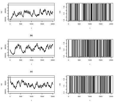
attracted in this region once it has entered. The computer simulations in Figure 5 support this result clearly.
We vary the values for the transition rates ν12 and ν21. Figure 6 shows how the different values of the
transition rates affect the behaviour of I(t). We notice that it takes longer to switch between the two states
when the transition rates are small, so I(t) is more likely to approach the boundaries.
0 500 1000 1500 2000
50000
65000
(a)
t
I(t)
0 500 1000 1500 2000
1.0
1.4
1.8
t
r(t)
0 500 1000 1500 2000
50000
65000
(b)
t
I(t)
0 500 1000 1500 2000
1.0
1.4
1.8
t
r(t)
0 500 1000 1500 2000
50000
65000
(c)
t
I(t)
0 500 1000 1500 2000
1.0
1.4
1.8
t
[image:26.612.89.476.125.473.2]r(t)
Figure 5: Computer simulation ofI(t) using the parameter values in Example 8.1 and its corresponding Markov
chain r(t), using formula (2.5) forI(t), with I(0) = 48500 for (a), I(0) = 60000 for (b) andI(0) = 76500 for
(c), and the exponential distribution for the switching times of r(t), with r(0) = 1. The horizontal lines in
the plot of I(t) indicate the levels α1
β1 and
α2
β2.
9
Summary
In this paper, we have introduced telegraph noise to the classical SIS epidemic model and set up the stochastic
SIS model. Note that the model assumes that the system switches between the two regimes and the Markov
switching is independent of the state of the system. Such an assumption is similar to that made in other
0 500 1000 1500 2000
50000
60000
70000
(a)
t
I(t)
0 500 1000 1500 2000
50000
60000
70000
(b)
t
[image:27.612.91.474.25.194.2]I(t)
Figure 6: Computer simulation of I(t) using the parameter values in Example 8.1, with ν12 = 0.6/day and
ν21 = 0.9/day for (a), and ν12 = 0.006/day and ν21 = 0.009/day for (b), using formula (2.5) for I(t) with
I(0) = 60000, and the exponential distribution for the switching times ofr(t), with r(0) = 1. The horizontal
lines in the plot of I(t) indicate the levels α1
β1 and
α2
β2 (which the values of I(t) never quite reach).
disease to spread faster or slower and switch between two or more regimes. In such a situation it is reasonable
to assume that the switching parameter does not depend on the state of the system. We have established the
explicit solution for the stochastic SIS model and also established conditions for extinction and persistence
of the disease. For the stochastic Markov switching model a threshold value TS
0 was defined for almost sure
persistence or extinction. We started with the special case in which the Markov chain has only two states and
then generalised our theory to the general case where the Markov chain has M states. Theorem 7.2 shows
that if T0S <1, the disease will die out. Theorem 7.3 shows that if T0S >1, then the disease will persist. We
also showed Theorem 7.5 that if TS
0 >1 the number of infectious individuals will enter (0∨(α1/β1), αM/βM)
in finite time, and with probability one will stay in the interval once entered, and moreover the number of
infectious individuals can take any value up to the boundaries of (0∨(α1/β1), αM/βM) but never reach them
(Theorems 7.6 and 7.7).
Forj= 1,2, . . . M, defineRD 0j =
βjN
µj+γj. Note that if αj >0 then R
D
0j >1 and
αj
βj
=N
1− 1
RD 0j
is the long-term endemic level of disease in the SIS model (1.4) with β =βj, µ=µj and γ =γj. If αj ≤0
then RD
0j ≤1 and disease eventually dies out in the same SIS model. Hence 0∨(α1/β1) is the smallest and
αM/βM is the largest long-term endemic level of disease in each of the M separate SIS models between which
the Markov chain switches.
We have not been able to prove extinction for the case whenTS
0 = 1, but the computer simulation shows
that the disease would die out after a long period of time, as we suspect. We have illustrated our theoretical
amongst young children.
Acknowledgements
The authors would also like to thank the Scottish Government, the British Council Shanghai and the Chinese
Scholarship Council for their financial support.
References
[1] Anderson, D.R., Optimal exploitation strategies for an animal population in a Markovian environment:
a theory and an example,Ecology 56, (1975), 1281-1297.
[2] Anderson, W.J., Continuous-Time Markov Chains, Springer-Verlag, Berlin-Heidelberg, 1991.
[3] Andersson, P. and Lindenstrand,D., A stochastic SIS epidemic with demography: initial stages and time
to extinction,J. Math. Biol. 62, (2011), 333-348.
[4] Artalejo, J.R., Economou, A. and Lopez-Herrero, M.J., On the number of recovered individuals in the
SIS and SIR stochastic epidemic models,Math. Biosci.228, (2010), 45-55.
[5] Bhattacharyya, R. and Mukhopadhyay, B., On an eco-epidemiological model with prey harvesting and
predator switching: Local and global perspectives, Nonlinear Anal.: Real World Appl. 11, (2010),
3824-3833.
[6] Brauer, F., Allen, L.J.S., Van den Driessche, P. and Wu, J.,Mathematical Epidemiology, Lecture Notes in
Mathematics, No. 1945, Mathematical Biosciences Subseries, Springer-Verlag, Berlin-Heidelberg, 2008.
[7] Brugger, S.D., Hathaway, L.J. and M¨uhlemann, K., Detection of Streptococcus pneumoniae strain
co-colonization in the nasopharynx,J. Clin. Microbiol. 47(6), (2009), 1750-1756.
[8] Caswell, H. and Cohen, J.E., Red, white and blue: Environmental variance spectra and coexistence in
metapopulations, J. Theoret. Biol. 176 (1995), 301-316.
[9] Coffey, T.J., Enright, M.C., Daniels, M., Morona, J.K., Morona, R., Hryniewicz, W., Paton, J.C. and
Spratt, B.G., Recombinational exchanges at the capsular polysaccharide biosynthetic locus lead to
fre-quent serotype changes among natural isolates ofStreptococcus pneumoniae,Mol. Microbiol.27, (1998),
73-83.
[10] Diekmann, O. and Heesterbeek, J.A.P., Mathematical Epidemiology of Infectious Diseases: Model
[11] Du, N.H., Kon, R., Sato, K. and Takeuchi, Y., Dynamical behaviour of Lotka-Volterra competition
systems: non autonomous bistable case and the effect of telegraph noise, J. Comput. Appl. Math. 170
(2004), 399–422.
[12] Farrington, P., What is the reproduction number for pneumococcal infection, and does it matter? in
4th International Symposium on Pneumococci and Pneumococcal Diseases, May 9-13 2004 at Marina
Congress Center, Helsinki, Finland, 2004.
[13] Feng, Z., Huang, W. and Castillo-Chavez, C., Global behaviour of a multi-group SIS epidemic model
with age-structure, J. Diff. Eqns. 218(2) (2005), 292-324.
[14] Gilpin, M.E., Predator-Prey Communities, Princeton University Press, Princeton, 1975.
[15] Gopalsamy, K., Stability and Oscillations in Delay Differential Equations of Population Dynamics,
Kluwer Academic, Dordrecht, 1992.
[16] Gray, A., Greenhalgh, D., Hu, L., Mao, X. and Pan, J., A stochastic differential equation SIS epidemic
model,SIAM J. Appl. Math. 71, (2011), 876-902.
[17] Hethcote, H.W., Qualitative analyses of communicable disease models,Math. Biosci.28 (1976), 335–356.
[18] Hethcote, H.W. and Yorke, J.A., Gonorrhea Transmission Dynamics and Control, Lecture Notes in
Biomathematics 56, Springer-Verlag, Berlin-Heidelberg, 1994.
[19] Hoti, F., Erasto, P., Leino, T. and Auronen, K., 2009, Outbreaks of Streptoccocus P neumoniae in day
care cohorts in Finland - implications for elimination of transmission,BMC Infectious Diseases 9 (2009),
102, doi:10.1186/1471-2334-9-102.
[20] Iannelli, M., Milner, F. A. and Pugliese, A., Analytical and numerical results for the age-structured SIS
epidemic model with mixed inter-intracohort transmission,SIAM J. Math. Anal.23(3) (1992), 662–688.
[21] Lamb, K.E., Greenhalgh, D. and Robertson, C., A simple mathematical model for genetic effects in
pneumococcal carriage and transmission,J. Comput. Appl. Math. 235(7) (2010), 1812–1818.
[22] Li, J., Ma, Z. and Zhou, Y., Global analysis of an SIS epidemic model with a simple vaccination and
multiple endemic equilibria,Acta Mathematica Scienta 26 (2006), 83–93.
[23] Lipsitch, M., Vaccination against colonizing bacteria with multiple serotypes, Proc. Nat. Acad. Sci.94
(1997), 6571-6576.
[24] Liu, X. and Stechlinski, P., Pulse and constant control schemes for epidemic models with seasonality,
Nonlinear Anal.: Real World Appl. 12, (2011), 931-946.
[25] Mao, X., Stability of Stochastic Differential Equations with Respect to Semimartingales, Longman