Modular modelling of combined AC and DC systems in dynamic simulations

This is a repository copy of

Modular modelling of combined AC and DC systems in

dynamic simulations

.

White Rose Research Online URL for this paper:

http://eprints.whiterose.ac.uk/105996/

Version: Accepted Version

Proceedings Paper:

Aristidou, P orcid.org/0000-0003-4429-0225, Papangelis, L, Guillaud, X et al. (1 more

author) (2015) Modular modelling of combined AC and DC systems in dynamic

simulations. In: PowerTech, 2015 IEEE Eindhoven. 2015 IEEE Eindhover PowerTech, 29

Jun - 02 Jul 2015, Eindhoven, Netherlands. IEEE . ISBN 978-1-4799-7693-5

https://doi.org/10.1109/PTC.2015.7232324

(c) 2015 IEEE. Personal use of this material is permitted. Permission from IEEE must be

obtained for all other users, including reprinting/ republishing this material for advertising or

promotional purposes, creating new collective works for resale or redistribution to servers

or lists, or reuse of any copyrighted components of this work in other works.

[email protected] https://eprints.whiterose.ac.uk/ Reuse

Items deposited in White Rose Research Online are protected by copyright, with all rights reserved unless indicated otherwise. They may be downloaded and/or printed for private study, or other acts as permitted by national copyright laws. The publisher or other rights holders may allow further reproduction and re-use of the full text version. This is indicated by the licence information on the White Rose Research Online record for the item.

Takedown

If you consider content in White Rose Research Online to be in breach of UK law, please notify us by

Modular modelling of combined AC and DC

systems in dynamic simulations

Petros Aristidou

Lampros Papangelis

Dept. of Elec. Eng. and Comp. Science, University of Li`ege, Belgium

{p.aristidou, l.papangelis}@ulg.ac.be

Xavier Guillaud

L2EP - Ecole Centrale de Lille, France

[email protected]

Thierry Van Cutsem

Fund for Scientific Research (FNRS) at Dept. of Elec. Eng. and Comp. Science,

University of Li`ege, Belgium

[email protected]

Abstract—A formulation is proposed in which an AC-DC system is modeled as a combination of AC grids, DC grids, injectors, AC two-ports and AC/DC converters, respectively. This modular modelling facilitates the dynamic simulation of future complex AC/DC systems. Furthermore, it can be exploited by the solver, which performs less operations on components with lower dynamic activity, and offers parallel processing of the time simulation. This approach is illustrated on a test system in which a multi-terminal DC grid connects two asynchronous AC systems, allows frequency support between them, and acts as emergency control against AC voltage instability.

Index Terms—Time simulation, phasor approximation, AC/DC systems, multi-terminal DC system, domain decomposition meth-ods, Schur complement, parallel processing.

I. INTRODUCTION

The increasing opening of electricity markets, the decom-missioning of traditional power plants, and the harvesting of sustainable energy from remote (in particular off-shore) locations will result in larger power transfers over longer distances. This imperative evolution of transmission grids, as well as the progress made in Voltage Source Converters (VSCs), has triggered a vibrant development of High-Voltage Direct Current (HVDC) systems [1], [2]. As a result, more and more HVDC interconnections are in operation or planned.

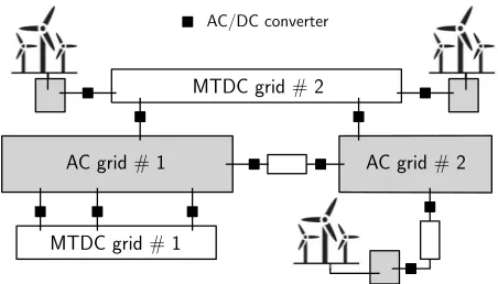
While point-to-point links have become very common [2], Multi-Terminal DC (MTDC) systems are the next step en-visaged [3], [4]. They will result in more complex HVDC network topologies. An illustrative example is sketched in Fig. 1 where AC grids are shown with gray boxes, and DC with white. The system includes two point-to-point HVDC links. One of them allows power exchange (and possibly frequency support) between the asynchronous AC systems #1 and #2. The other link connects a wind park to AC system #2. The overlay MTDC grid #1 serves as a backbone reinforcing AC system #1 by offering an alternative path for power transfers between remote locations inside that system. The MTDC grid #2 collects the energy produced by two off-shore wind parks but also allows power transfers between the AC systems #1 and #2. The generators within each wind park are connected through AC cables which make up a separate AC grid. The latter can be modeled in detail or replaced by a single, isolated AC bus if the generators are lumped into one equivalent.

AC grid # 1 AC grid # 2

MTDC grid # 2

MTDC grid # 1

AC/DC converter

Figure 1: Illustrative example of combined AC-DC system

In the future, the need for dynamic simulation of combined AC and DC systems will keep increasing [5]. For instance, HVDC systems are expected to take a greater part in frequency and voltage control [6]. Furthermore, the response of AC/DC converters to nearby faults in AC grids must be taken into account when assessing system security.

To reproduce the dynamics of AC/DC converters, Electro-Magnetic Transient (EMT) simulation remains the reference in terms of accuracy. However, the EMT models are not suited to the large-scale studies and long-term dynamics considered in this paper, for which the phasor approximation is preferred. To anticipate the future developments, while accommodat-ing the above mentioned diversity of HVDC system topolo-gies, there is a need for a flexible AC-DC system dynamic modelling. Models of point-to-point HVDC links have been available for quite some time in industry-grade dynamic sim-ulation software [7]. While their developers certainly work to-wards incorporating MTDC systems, there are, to the authors’ knowledge, few publications devoted to such developments.

This paper proposes a modular formulation making it easy to develop, extend and maintain models for an MTDC topol-ogy of arbitrary complexity.

New-ton iterations on components with lower participation in the dynamic response. It also paves the way to parallel processing of the computations to further accelerate the simulations.

These features are present in RAMSES, a research software developed at the University of Li`ege [8], whose results are presented in this paper.

II. MODULAR MODELLING OF ANAC-DCSYSTEM

A. AC and DC transmission sub-networks

Modular modeling is built upon the concept of the trans-mission grid being an arbitrary combination of (disjoint) AC and DC sub-networks. In the case of Fig. 1, for instance, the transmission grid can be considered to include five AC and four DC sub-networks.

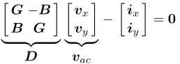
Under the phasor approximation, AC networks are repre-sented by the well-known algebraic equations:

[

G−B

B G

]

| {z } [

vx

vy

]

| {z } −

[

ix

iy

]

=0

D vac

(1)

where G (resp. B) is the nodal conductance (resp.

suscep-tance) matrix, vx and vy are vectors of real and imaginary

components of the bus voltage, and ix andiy are the

corre-sponding injected current components.

Similarly, by neglecting the series inductances of DC lines and cables, and accounting for their shunt capacitances in the AC/DC converters [9], the DC grid is represented by a network of resistances, modelled by:

Gdcvdc−idc=0 (2)

whereGdcthe nodal conductance matrix,vdcis the vector of

DC bus voltages, andidc the vector of injected DC currents.

This encompasses any AC-DC grid topology. If there are

several disjoint AC sub-networks, theGandBmatrices have

a block-diagonal structure. The same holds true for Gdc in

case of disjoint DC sub-networks. In the system of Fig. 1, for

instance, G andB have five nonzero diagonal blocks, while

Gdchas four such blocks.

B. Equipment connected to AC or DC grids

Modularity is also obtained by matching any equipment connected to the AC or DC grids with one of the following three generic components:

• an injector connected to a single AC bus • an AC two-portconnecting two AC buses

• anAC/DC converterconnecting one AC and one DC bus. Each component is modelled by a system of Differential-Algebraic Equations (DAEs). Including algebraic equations and states offers remarkable modelling flexibility. In particular, each component model interfaces with the network through the currents injected into it, involved in the DAEs as algebraic states. This allows processing the components separately dur-ing the simulation, as mentioned in the Introduction.

Each of the above three generic components is considered hereafter in some more detail, with reference to Fig. 2.

vxkvyk

ixjiyj

xj

j-th injector xj

vxkvyk vxℓvyℓ

j-th AC two-port

ixoj iyoj ixej iyej

AC grid AC grid

AC grid DC grid

vxkvyk ixj iyj idcj vdcℓ

j-th AC/DC converter

xj =

∼

Figure 2: The three generic components

C. Injector

Synchronous machines, synchronous condensers, static var compensators, motors, static loads, wind-turbine generators,

etc. are well-known examples of injectors. The j-th injector

attached to thek-th AC bus is modelled by:

Γ_jx˙j =Φj(xj, vxk, vyk) (3)

wherexjis a state vector including both differential and

alge-braic variables,vxk andvyk are the bus voltage components.

In this and subsequent models, Γ_{j is a diagonal matrix with}

(Γ_{j)ℓℓ= 0if theℓ-th equation is algebraic, and one otherwise.}

The use of Γ_{j provides additional modelling flexibility to}

handle nonlinearities by changing a differential equation into an algebraic one during the simulation, and conversely [10].

Formally this corresponds to changing a diagonal entry ofΓ_j

from one to zero, and conversely. This feature is available in the solver of RAMSES.

Note that xj includes in particular the components of the

current injected in the connection bus, i.e.xj= [ixjiyj . . .]T.

D. AC two-port

While an injector is attached to a single AC bus, an AC two-port is aimed at connecting two AC buses. Thus, the generic

model ofj-th AC two-port connected to thek-th andl-th AC

buses is:

Γ_jx˙_{j =}Φ_{j(xj, vxk, vyk, vxl, vyl) (4)}

xj includes the components of the currents injected in both

AC buses, i.e.xj = [ixojiyoj ixej iyej . . .] T

where subscript

odenotes the origin and ethe extremity.

E. AC/DC converter

An AC/DC converter connects one AC with one DC bus.

Thus, thej-th AC/DC converter connecting the k-th AC bus

and thel-th DC bus is modelled by:

Γ_jx˙_{j =}Φ_{j(xj, vxk, vyk, vdcl) (5)}

where vdcl is the DC bus voltage. xj includes the current

components: xj = [ixjiyj idcj . . .] T

.

III. SOLUTION ALGORITHM

Let the AC network equations (1) be rewritten as:

0_=Dvac− N

∑

j=1

Cjxj ,gac(x,vac) (6)

where N is the total number of injectors, AC two-ports and

AC/DC converters in the system.Cjis a matrix with zeros and

ones whose purpose is to extract the AC current components

from the various xj state vectors and add them to the proper

network equations.

Similarly, the DC network equations (2) are rewritten as:

0₌Gdcvdc− Ndc

∑

j₌₁

Ejxj,gdc(x,vdc) (7)

where Ndc is the number AC/DC converters, andEj is also

a matrix with zeros and ones.

For the purpose of numerical simulation, the DAE systems (3), (4) and (5) are algebraized using a differentiation formula, such as Trapezoidal Rule or Backward Differentiation Formula (BDF). This yields the algebraized equations in compact form:

0_{=fj(xj,vac,vdc), j= 1, . . . , N. (8)}

At each discrete time tm the nonlinear equations (8) are

solved together with the AC-DC network equations (6, 7) using

a Newton method to obtain the vectors xj(tm),vac(tm)and

vdc(tm). At the k-th Newton iteration, the following linear

equations have to be solved (j= 1, . . . , N):

Aj∆xkj +

[

Bj Hj

][∆vack

∆vk dc

]

=−fj(xkj−1,v k−1

ac ,v k−1

dc ) (9)

D∆vack − N

∑

j=1

Cj∆xkj =−gac(xk−1,vkac−1,v k−1

dc ) (10)

Gdc∆vkdc− Ndc

∑

j=1

Ej∆xkj =−gdc(xk−1,vkac−1,v k−1

dc ) (11)

where ∆ denotes a vector correction, Aj is the Jacobian of

thej-th component towards its state variablesxj,Bj towards

vac andHj towardsvdc.

The above equations are solved in a decomposed way by reorganizing them as follows. The injector, the AC two-port

and the AC/DC converter state vector corrections ∆xk

j are

obtained from Eqs. (9) and introduced in Eqs. (10) and (11), to obtain the Schur-complement system of Eq. (12) (see next page). Then, at each Newton iteration, the latter system is

solved to obtain the voltage corrections∆vk

acand∆vdck which

are substituted in the various sets of equations (9). The latter

are then solved to obtain the state corrections ∆xk

j.

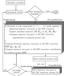
This procedure removes the data dependencies between the various components, allowing their respective sets of equations to be solved independently. In fact, both the modular modelling and the Schur-complement formulation allow many calculations associated with injectors, AC two-ports or AC/DC converters to be performed independently of each other: DAE

Parallel threads

Parallel threads

(N+1 parallel tasks)

(N parallel tasks)

Figure 3: Decomposed and parallelized simulation algorithm

system discretization, Jacobian and Schur-complement compu-tation, matrix factorization, linear system solution, etc. Thus, shared-memory parallel computing techniques are employed to accelerate the dynamic simulation as shown in Fig. 3.

As is well-known, the D and Gdc matrices have a very

sparse structure, inherited from the sparse nodal admittance matrix. As explained hereafter, sparsity is very little affected

by the elimination of the ∆xk

j variables. Hence, the

Schur-complement matrix in the left hand side of Eq. (12) is also very sparse, allowing fast network solutions.

It has to be noted first thatBj andHj are extremely sparse

matrices. For an injector, since the model involves only two

AC voltage components (vxk,vyk), only two columns ofBj

are non-zero, corresponding to the positions of vxk and vyk

invac. Similarly, for an AC two-port,Bj includes four

non-zero columns while, for an AC/DC converter,Bjincludes two

non-zero columns andHj one.

From the sparsity patterns of matricesCjandBj, it can be

shown that theCjA−j1Bjcontribution of an injector has only

four non-zero elements which modify four, already non-zero,

elements ofD, corresponding tovxk andvyk. Those elements

are shown with squares in Fig. 4.

Similarly, the CjA−j1Bj contribution of an AC two-port

consists of sixteen nonzero elements. Eight of them modify

already nonzero entries of a diagonal sub-matrix ofD,

corre-sponding tovxk,vyk,vxlandvyl. The other eight, off-diagonal

       [ D 0

0 _Gdc ] +        N ∑ j

CjA−j1

[

BjHj

]

Ndc

∑

j

EjA−j1

[

BjHj

]               [

∆vac

∆vdc

] =       

−gac(xk−1,vack−1,v k−1

dc )− N

∑

j

CjA−j1fj(xkj−1,v k−1

ac ,v k−1

dc )

−gdc(xk−1,vack−1,v k₋₁ dc )−

Ndc

∑

j

EjA−j1fj(xkj−1,v k−1

ac ,v k₋₁ dc )        (12)

Figure 4: Contribution of injectors and AC/DC converters to the Schur-complement matrix in the left-hand side of Eq. (12)

Finally, the CjA−j1Bj, CjAj−1Hj, EjA−j1Bj and

EjA−j1Hj matrices of an AC/DC converter contribute with

nine nonzero elements. They modify four, already nonzero,

elements of D corresponding to vxk, vyk as well as one

element of Gdc corresponding to vdcl. Those five terms are

shown with squares and cross in Fig. 4. The remaining four contributions correspond to couplings between these variables; they are shown with disks in Fig. 4.

Obviously, sparse matrix storage is used for D, Gdc,Bj,

Ej,CjandHjwhose sparsity patterns are known beforehand

from the network topology. Only the nonzero elements of each correction term are computed, by solving linear systems with

coefficient matricesAj.

Last but not least, the Jacobian matrices are updated in-frequently and kept constant over several Newton iterations or even discrete time steps. They are updated only if convergence has not taken place after a number of Newton iterations at the same discrete time-step.

IV. SIMULATION RESULTS

A. Test system

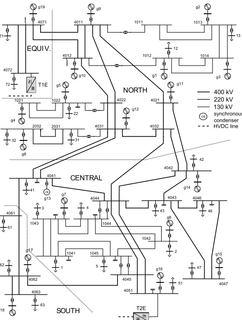
The system shown in Figs. 5 and 6 was modeled as described in Section II and simulated with the algorithms of Section III. It consists of two asynchronous AC systems and one offshore wind farm, connected through a five-terminal HVDC grid equipped with five VSCs.

The “East” AC system is based on the so-called Nordic test system. The starting point was the variant documented in [11], at its insecure operating point A. With respect to [11], the system was modified as follows:

• the large, equivalent generator connected to bus 4072 was

removed and replaced by the T1E converter;

• another connection to the DC grid was added at bus 4051,

through the T2E converter. This allows using the MTDC system as an overlay grid reinforcing the AC system.

≃

=

≃

=

≃

=

≃

=

NORDIC WEST NORDIC EAST

T1W T1E T2W T2E

≃

=

See Fig. 6 (op. point A in [11] See Fig. 6

(op. point B in [11])

Figure 5: Overall structure of the test system

g11 g19 g16 g17 g18 g2 g9 g1 _g3 g10 g5 g4 g12 g8 g13 g14 g7 g6 g15 4011 4012 1011 1012 1014 1013 1022 1021 2031 cs 4046 4043 4044 4032 4031 4022 4021 4071 4072 4041 1042 1045 1041 4063 4061 1043 1044 4047 4051 4045 4062 NORTH CENTRAL EQUI V. SOUTH 4042 2032 1 5 2 3 4 63 62 61 51 47 42 41 31 32 22 12 13 71 72 46 43 400 kV 220 kV 130 kV synchronous condenser cs T2E T1E HVDC line

Figure 6: Nordic test system with HVDC grid connections

The “Nordic West” system is a mirror copy of its East counterpart, but operating at the secure point B documented in [11]. It is connected to the DC grid through T1W and T2W. The Wind Farm is modeled through a simple two-bus AC grid connected through the TWF converter (see Fig. 5).

The modelling of Section II yields a 5 ×5 matrix G_dc,

while matrices G_andB _{have three nonzero diagonal blocks}

corresponding to the East, West and WF grids, respectively. The five AC/DC converters, of the VSC type, are modeled in detail, as recommended in [3], [9], [12]. The TWF converter imposes constant voltage and frequency on the AC side, thus acting as a slack bus. The other four converters operate in voltage-droop mode. Thus, when the wind farm output changes, the current collected by TWF varies and the resulting power change is shared by T1E, T2E, T1W and T2W.

Last but not least, these four VSCs are provided each with the frequency support control proposed in [13]. Then the

controller uses the local frequency measurement f as input,

and outputs a correction which is added to the active power set-point of the VSC, together with the voltage droop term. The control becomes active when frequency leaves a predefined

deadband. Then, through integral control, the active powerP

in the VSC is forced to follow in steady-state aP−f droop

characteristic, similar to the speed droop characteristic of a conventional speed governor.

B. Scenario and system response

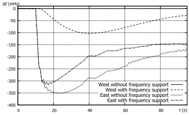
The example reported here involves frequency support be-tween AC systems, as well as an emergency control with the HVDC grid stabilizing the AC system in the long term. The initial event is the outage of generator g17 in the East system. This disturbance causes the frequency drop shown in Fig. 7. Without frequency support, the East frequency drops by 350 mHz, while the West frequency remains unaffected. With frequency support, the controllers present in T1E and T2E activate the help of the East system by the West one by actuating a power transfer through the HVDC grid. This is triggered when frequency drops by more than 200 mHz, which

is sensed by the T2E converter at t = 1.2 s and by T1E at

t= 1.4s. The benefit of this control is to reduce the frequency

drop in the East system to 300 mHz, while the West system frequency undergoes a moderate variation, as shown in Fig. 7. Att= 100s, the frequency support control is automatically deactivated when the East frequency has recovered [13].

The system recovers but, in the long term, under the effect of LTCs attempting to restore distribution voltages and OverExci-tation Limiters (OELs) bringing generator field currents below their limits, voltage instability takes place and the system

eventually collapses at t ≃ 120 s, as shown in Fig. 8. This

instability results from the increased power transfer in the lines between the North and Central areas (see Fig. 6) when the production lost in the Central area is compensated by the generators in the North [11]. With the frequency support control, the power injected by T2E somewhat relieves those lines and yields a slightly better, but still unstable voltage evolution, as shown by the dashed curve in Fig. 8.

-400 -350 -300 -250 -200 -150 -100 -50 0

0 20 40 60 80

Δf (mHz)

t (s) West without frequency support

West with frequency support East without frequency support East with frequency support

Figure 7: Frequency deviations in East and West systems

To relieve those lines, a remedial action consists of trans-ferring power from North to Central areas through the HVDC

grid. To this purpose, fromt= 120to140s, the active power

set-point of T1E is ramped down by 200 MW while that of

T2E is ramped up by the same amount. The resulting voltage stabilization is easily seen from Fig. 8.

The evolution of VSC active powers and DC voltages including both remedial actions, are shown in Figs. 9 and 10, respectively. During the frequency support period, DC voltages drop due to the power request that draws on the energy stored in the DC capacitors. This is promptly compensated by the VSC controls, and the DC voltages settle to values dictated by the voltage droop settings of T1W and T2W. By properly tuning the frequency support controller, the overshoot in the active power response of T1E and T2E, and the DC voltage depletion are very limited [13]. The power ramping of T1E and T2E to stabilize voltages in the long term is easily seen in Fig. 9. The power changes in T1W and T2W are negligible, and the power transfer from West to East remains unchanged.

V. PROFILING THE MODULAR SOLVER PERFORMANCE

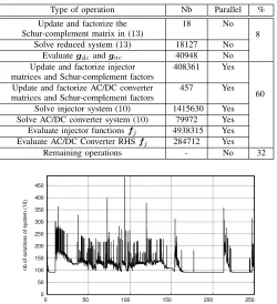
Table I lists the major operations performed during the whole simulation until the system returns to steady state. The

step size used is 20 ms. It also shows which of them are

performed in parallel and the percentage of the execution time in the parallel or sequential sections, respectively. The remaining time is spent on handling the time-step initializa-tion, bookkeeping, output of computed values, etc.

It can be seen that the time spent to update, factorize and solve the reduced system (12) is small compared to the overall simulation time. This is due to the infrequent update

of the Schur-complement matrix (only 18 times throughout

the simulation) and to the sparsity of the matrix which allows employing fast, sparse linear solvers. The largest percentage of the simulation time is spent on updating, factorizing and solving the injector and AC/DC converter systems (9). Fig-ure 11 shows the total number of solutions performed at every time step. It can be seen that the number of solutions spikes after major events (generator tripping, OEL action, activation of controls, etc.).

0.75 0.8 0.85 0.9 0.95 1

0 40 80 120 160 t (s)

V (pu)

VSC2E and VSC3E setpoints change

No emergency controls Only frequency support Frequency support and emergency control

Figure 8: Voltage at bus 1041

-300 -200 -100 0 100 200 300

0 40 80 120 160 t (s)

P(MW)

TWF T1E T1W T2E T2W

Figure 9: Active power of VSCs

0.96 0.965 0.97 0.975 0.98 0.985 0.99 0.995 1

0 40 80 120 160

Vdc (pu)

t (s) Bus TWF

Bus T1E Bus T2E Bus T1W Bus T2W

Figure 10: DC voltages

Table I:Major operations over the entire simulation

Type of operation Nb Parallel %

Update and factorize the Schur-complement matrix in (13₎

18 No

8 Solve reduced system (13_{) 18127 No}

Evaluategdcandgac 40948 No Update and factorize injector

matrices and Schur-complement factors

408361 Yes

60 Update and factorize AC/DC converter

matrices and Schur-complement factors

457 Yes

Solve injector system (10) 1415630 Yes Solve AC/DC converter system (10_{) 79972 Yes} Evaluate injector functionsfj 4938315 Yes Evaluate AC/DC Converter RHSfj 284712 Yes

Remaining operations - No 32

0 50 100 150 200 250 300 350 400 450

0 50 100 150 200 250

nb of solutions of system (10)

Figure 11: Number of systems (9) relative to injectors and AC/DC

converters solved at each time step

execution takes 5.2 s, while a simulation in parallel using the

four cores takes 3.7 s. That is, the simulation is 1.41 times

faster, even on this small test system, and using a standard

computer. Overall, as 60% of the operations are performed

in parallel, and by ignoring any parallelization overhead and

imbalances, the computation can be up to 2.5 times faster

compared to a sequential run of the same algorithm.

It is noteworthy that even the sequential execution of the algorithm is very fast as it takes advantage of the modularity to update and compute the injectors and the AC/DC converters asynchronously, only when needed.

VI. CONCLUSION

A modular modelling has been proposed allowing to handle AC and DC network topologies of virtually any complexity. To this purpose, the system is seen as a combination of AC grids, DC grids, injectors, AC two-ports and AC/DC converters,

respectively.

This modularity is exploited by the solver, which performs less operations on components with lower dynamic activity, and offers parallel processing of the time simulation. This is made possible by a Schur-complement-based decomposition allowing to solve the equations of the above mentioned com-ponents separately, with asynchronous update of Jacobians. The sparsity of the involved matrices is exploited extensively. The approach has been illustrated on a test system in which a multi-terminal DC grid allows frequency support between asynchronous AC grids, and provides emergency control against AC voltage instability. In spite of the small system size, the results confirm the advantages of the proposed modelling and computational procedure.

REFERENCES

[1] “Ten year network development plan 2010-2020,” tech. rep., ENTSO-E, 2010.

[2] CIGRE Tech. Brochure JWG C4/B4/C1.604, Influence of Embedded HVDC Transmission on System Security and AC Network Performance, 2013.

[3] P. Rault, X. Guillaud, F. Colas, and S. Nguefeu, “Method for small signal stability analysis of VSC-MTDC grids,” inProc. of IEEE PES General Meeting, 2012.

[4] D. Van Hertem and M. Ghandhari, “Multi-terminal VSC HVDC for the European supergrid: Obstacles,”Renewable and Sustainable Energy Reviews, vol. 14, no. 9, pp. 3156–3163, 2010.

[5] J. Beerten, O. Gomis-Bellmunt, X. Guillaud, J. Rimez, A. van der Meer, and D. Van Hertem, “Modeling and control of hvdc grids: A key challenge for the future power system,” inProc. of PSCC, 2014. [6] “Entso-e draft network code on high voltage direct current connections

and dc connected power park modules,” 2014.

[7] S. Cole and B. Haut, “Robust modeling against model-solver interactions for high-fidelity simulation of VSC HVDC systems in EUROSTAG,” IEEE Trans. on Power Systems, vol. 28, no. 3, pp. 2632–2638, 2013. [8] P. Aristidou, D. Fabozzi, and T. Van Cutsem, “Dynamic simulation of

large-scale power systems using a parallel Schur-complement-based de-composition method,”IEEE Trans. on Parallel and Distributed Systems, vol. 25, no. 10, pp. 2561–2570, 2014.

[9] S. Cole and R. Belmans, “A proposal for standard VSC HVDC dynamic models in power system stability studies,” Electric Power Systems Research, vol. 81, no. 4, pp. 967–973, 2011.

[10] D. Fabozzi, A. S. Chieh, P. Panciatici, and T. Van Cutsem, “On simplified handling of state events in time-domain simulation,” inProc. of PSCC, 2011.

[11] T. Van Cutsem and L. Papangelis, “Description, modeling and simulation results of a test system for voltage stability analysis,” internal report, University of Li`ege, 2013. http://hdl.handle.net/2268/141234. [12] M. Imhof and G. Andersson, “Dynamic modeling of a VSC-HVDC