Local abstraction refinement for probabilistic timed programs

Contents lists available atScienceDirect

Theoretical Computer Science

www.elsevier.com/locate/tcs

Local abstraction refinement for probabilistic timed programs

Klaus Dräger

a,

∗

, Marta Kwiatkowska

a

, David Parker

b

, Hongyang Qu

a

a_{Department of Computer Science, University of Oxford, Oxford, UK} b_{School of Computer Science, University of Birmingham, Birmingham, UK}

a r t i c l e

i n f o

a b s t r a c t

Keywords:

Probabilistic verification Abstraction refinement

We consider models of programs that incorporate probability, dense real-time and data. We present a new abstraction refinement method for computing minimum and maximum reachability probabilities for such models. Our approach uses strictly local refinement steps to reduce both the size of abstractions generated and the complexity of operations needed, in comparison to previous approaches of this kind. We implement the techniques and evaluate them on a selection of large case studies, including some infinite-state probabilistic real-time models, demonstrating improvements over existing tools in several cases.

©2013 Elsevier B.V. All rights reserved.

1. Introduction

Abstraction refinement is a highly successful approach to the verification of complex infinite-state systems. The basic idea is to construct a sequence of increasingly precise abstractions of the system to be verified, with each abstraction typically over-approximating its behaviour. Successive abstractions are constructed through a process of refinement which terminates once the abstraction is precise enough to verify the desired property of the system under analysis. Abstraction refinement techniques have also been used to verify probabilistic systems[6,11,13,7], including those with real-time characteristics[16,

17,8]and continuous variables[25]. Frequently, though, practical implementations of these techniques are hindered by the

high complexity of both the abstractions involved and the operations needed to construct and refine them.

In this paper, we target the verification of programs whose behaviour incorporates both probabilistic and real-time aspects, and which include the manipulation of (potentially infinite) data variables. We analyse systems modelled as prob-abilistic timed programs (PTPs) [17], whose semantics are defined as infinite-state Markov decision processes (MDPs). We introduce an abstraction refinement procedure for computing minimum and maximum reachability probabilities in PTPs. As

in[6,11], we use an MDP-based abstraction. This providesouterbounds on reachability probabilities (i.e., a lower bound on

the minimum probability or an upper bound on the maximum). In addition, we compute dual,inner bounds, based on a stepwise concretisation of adversaries of this abstract MDP, yielding upper and lower bounds on minimum and maximum probabilities, respectively. Concretisation is also used, for example, in[11], for untimed models. The key difference in our work is that we aim to keep the abstraction small by usinglocalrefinement and simplification operations, so as to reduce the need for expensive operations such as Craig interpolation.

At the core of our approach is a refinement loop that repeatedly attempts to construct a concrete adversary of the PTP. This is based on the exploration of the part of the state space on which the current abstract adversary can be concretised. In each exploration step, we may encounter an inconsistency, in which case we derive a refinement operation and restart. Otherwise, we numerically solve the constructed adversary, giving inner bounds on the desired probability values. The refinement loop terminates once the difference between upper and lower bounds is smaller than a specified threshold

ε

.

*

Corresponding author.

E-mail address:klaus.draeger@cs.ox.ac.uk(K. Dräger).

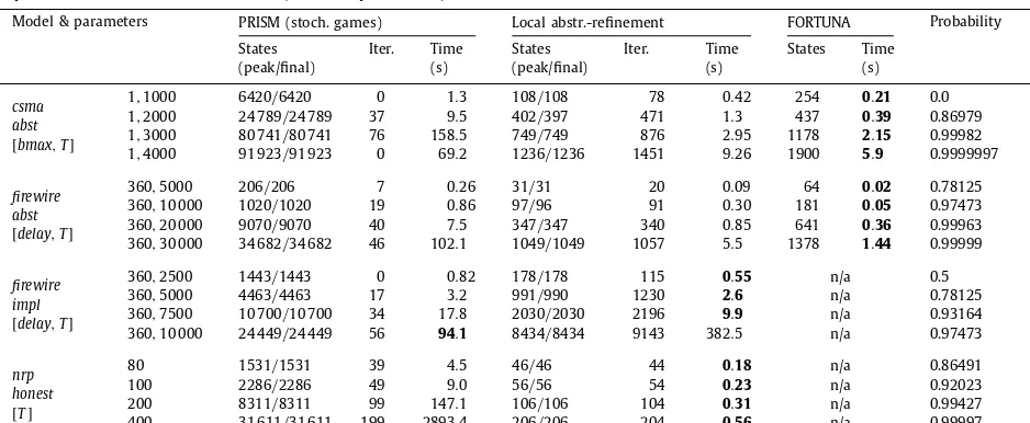
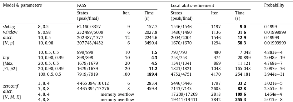
We implement our abstraction refinement approach, deploy it on various large case studies, and compare to the proba-bilistic verification tools PRISM [18], PASS [9]and FORTUNA[3], illustrating improved performance in many cases. We are also able to verify probabilistic timed programs containing both real-time behaviour and infinite data variables, which these tools cannot handle.

1.1. Related work

Abstraction refinement for MDPs and related models is an active research field. In [6], techniques were proposed for abstracting MDPs using the notion of probabilistic simulation. Building on the same approach to abstraction,[11]developed a probabilistic version of the classic counterexample-guided abstraction refinement (CEGAR) method, which was then im-plemented in the tool PASS[9]. This verifies a probability-bounded reachability property using a refinement scheme based on probabilistic counterexamples and Craig interpolation. In contrast to the implementation of[6], PASS uses predicate ab-straction, allowing it to analyse infinite-state models. More recent work[15] proposes an alternative probabilistic CEGAR technique using stochastic tree counterexamples; this applies to finite-state MDPs, on which properties are specified us-ing simulation rather than reachability. However, all three methods[6,11,15]were applied to discrete-time models (MDPs), whereas our approach generalises to models with real-time behaviour. We provide an experimental comparison with PASS, for MDP models, in Section4.

In [13], a quantitative abstraction refinement technique for MDPs was proposed, using a different form of abstraction based on stochastic games. This computes lower and upper bounds for reachability probabilities, the difference between which determines if further refinement is needed. The framework of [13] was subsequently applied to verification of C programs with probabilistic behaviour [12]. Later extensions to PASS also use game-based abstraction refinement[24]. In recent work[7], the abstraction frameworks of[13,24]were adapted to handle arbitrary abstract domains, illustrating cases where this can outperform predicate abstraction. As for[6,11,15]above, though, these methods [13,12,24,7] all focus on models with a discrete notion of time.

Probabilistic timed automata (PTAs) are a subclass of the probabilistic timed programs (PTPs) that we target in this paper, since only the latter allows arbitrary (infinite) data variables. For PTAs, several verification techniques exist. Most relevant here is [16], which extends the abstraction refinement framework of [13] mentioned above, to PTAs, by using zones to represent abstract states. Other possibilities include the digital clocks discretisation[19]and backwards reachability[21]. The probabilistic model checker PRISM[18]supports verification of PTAs, using either[16]or[19]. In[16], abstraction refinement was shown to outperform the other available techniques. Subsequently, an optimised version of backwards reachability, implemented in the tool FORTUNA[3], was shown to exhibit superior performance on various examples. We compare the performance of our approach to both PRISM and FORTUNA in Section4.

Several PTA verification tools do support PTAs with data variables, but they are required to be finite. This includes PRISM, discussed above,

mcpta

[10], which translates the modelling language Modest to PRISM using[19], and UPPAAL PRO, which computes maximum reachability probabilities for PTAs by progressively partitioning the state space into sets of zones.

The closest approaches to the one presented here are[17]and[8]. In[17], an extension of the game-based abstraction refinement framework of [13] is defined for PTPs, but not implemented. This defines abstractions as stochastic games, rather than MDPs as in our approach. In recent work [8], PTPs (there called variable-decorated PTAs) are verified using a combination of discretisation via digital clocks [19] and predicate abstraction methods from PASS [24]. Our approach avoids the use of discretisation by using zones and aims to improve efficiency by using local refinement and simplification operations to reduce the size of abstractions. The implementation of [8]is not currently available; we give a brief, indirect comparison of results in Section4.

2. Preliminaries

We assume a set

V

ofvariables, ranging over a domainD defined by a theory T (linear integer arithmetic in our exam-ples). We require satisfiability of quantifier-free formulae inT to be decidable. The set ofassertionsover

V

, i.e., (conjunctive) quantifier-free formulae in T, is denoted byAsrt

(

V

)

, andVal

(

V

)

is the set ofvaluationsof

V

, i.e., functionsu

:

V

→

D. We useAssn

(

V

)

for the set ofassignmentsover

V

, given by a termrx for eachx

∈

V

. The result of applying assignment f to a valuation u is f

(

u

)

, given for each x

∈

V

by f

(

u

)(

x

)

=

u

(

rx

)

. Given an assignment f and an assertion

ϕ

, the composition

ϕ

◦

f is defined by

(

ϕ

◦

f

)(

u

)

≡

ϕ

(

f

(

u

))

.

For a set S, we use

P

(

S

)

to denote the set of subsets ofSand

D

(

S

)

for the set of discrete probability distributions overS, i.e. finite-support functions

:

S

→ [

0

,

1

]

such that

_s∈S

(

s

)

=

1. A distribution

∈

D

(

S

)

with support

{

s1

, . . . ,

sn

}

and

(

sj

)

=

λ

j will also be written

λ

1s1

+ · · · +

λ

nsn.

2.1. Clocks

We use a set

X

of clock variables to represent the time elapsed since the occurrence of various events. The set of

clock valuationsis

R

X₀

= {

v

:

X

→

R

0

}

. For any clock valuationv and

δ

∈

R

0, thedelayedvaluation v

+

δ

is defined by

(

v

+

δ)(

x

)

=

v

(

x

)

+

δ

for allx

∈

X

. For a subsetY

⊆

X

, the valuationv

[

Y

:=

0

]

is obtained by setting all clocks inY to 0, i.e.,

Aclock difference constraintover

X

is an upper or lower bound on either a clock or the difference between two clocks. It is convenient to extend

X

with a dedicatedzero clock x0which is always 0, so that all clock difference constraints have the formx

−

y

bwithx

,

y

∈

X

0

:=

X

∪ {

x0

}

,

∈ {

<,

}

andb

∈

Z

∪ {±∞}

. We define thecomplement cof a clock difference constraintc as:c

:=

y

−

x

<

−

b ifc

≡

x

−

y

b; andc

:=

y

−

x

−

b ifc

≡

x

−

y

<

b.

A (convex)zoneis the set of clock valuations satisfying a number of clock difference constraints, and the set of all zones isZones

(

X

)

. We use several standard operations on zones:

•

future:

ρ

= {

v

+

δ

|

v

∈

ρ

, δ

∈

R

0

}

is the set of clock valuations reachable from

ρ

by letting time pass;

•

past:

ρ

= {

v

|

v

+

δ

∈

ρ

for some

δ

∈

R

0

}

is the set of clock valuations from which

ρ

can be reached by letting time pass;

•

clock reset: ifY

⊆

X

, then

ρ

[

Y

:=

0

] = {

v

[

Y

:=

0

] |

v

∈

ρ

}

contains the valuations obtained from

ρ

by setting the values of ally

∈

Y to 0;

•

inverse reset: ifY

⊆

X

, then

[

Y

:=

0

]

ρ

= {

v

|

v

[

Y

:=

0

] ∈

ρ

}

contains the valuations which end up in

ρ

if the values of all y

∈

Y are set to 0.

We will use one additional operation on clocks, for which we first require some standard operations on pairs

(

b

,

)

∈

R

0

× {

<,

}

(see[2]). The set

{

<,

}

is ordered by

<

, and the set of pairs

(

b

,

)

by the lexicographic combination

≺

of

<

_R and

, i.e.

(

b1

, <)

≺

(

b1

,

)

≺

(

b2

, <)

for allb1

<

b2. The sum of two pairs is then given by

(

b1

,

1

)

+

(

b2

,

2

)

:=

(

b1

+

b2

,

min

(

1

,

2

))

.

Definition 1.Let

ρ1

, . . . ,

ρ

m be zones whose intersection

ρ1

∩ · · · ∩

ρ

m is empty. Anunsatisfiable corefor

ρ1

, . . . ,

ρ

mis a set

C of constraints such that:

(i) each constraint inC is implied by some

ρ

k,

(ii) the conjunction of all constraints inC is unsatisfiable, and

(iii) C is minimal in the sense that no proper subsetC

Csatisfies (ii).

An unsatisfiable core always exists, since the zones are given by finite sets of constraints whose unionU is unsatisfiable (otherwise the zones would have a non-empty intersection), and the subsets of U satisfy the descending chain condition. We can compute an unsatisfiable core with the following straightforward generalisation of the Craig interpolation procedure for difference logic from[5].

For alli

,

j, let

(

bi j

,

i j

)

be the least pair for whichci j

≡

xi

−

xj

i jbi j is implied by some

ρ

k. Note that the conjunction of theci j is unsatisfiable. This means that, if we label the edges of the complete directed graph on

X

0 with the pairs

(

bi j

,

i j

)

, then there is a cycle with a negative label sum[2]; using the Floyd–Warshall algorithm, we can find a shortest such cycle

(

i1

, . . . ,

ik

)

.

The constraints along this cycle are xij−1

−

xij

ij−1ijbij−1ij for j

=

1

, . . . ,

k, wherei0

=

ik; the label sum

(

b

,

)

being negative means that summing the constraints results in an unsatisfiable implied constraint 0

b. On the other hand, re-moving one of the constraints (w.l.o.g., we can assume it is the first one) gives a path whose associated constraints are satisfied by any clock valuationt of the form v

(

xij

)

=

a

+

bi1i2

+ · · · +

bij−1ij for some large enough a. So the constraints along the cycle form an unsatisfiable core.

2.2. Markov decision processes (MDPs)

The underlying semantics for the models studied in this paper is defined in terms ofMarkov decision processes(MDPs), a standard model for systems with both probability and nondeterminism. An MDP is a tuple

(

S

,

si

,

Se

,

T

)

, where S is a (possibly infinite) set of states,si

∈

Sis the initial state,Se

⊆

Sis a set of error states andT

:

S

→

P

(

D

(

S

))

is a probabilistic transition function. In a states

∈

S, the choice of a successor distribution

∈

T

(

s

)

is nondeterministic and a successor state is then selected probabilistically according to

.

Anadversaryfor an MDP resolves the nondeterminism in each state, based on the current history, i.e., it is a function

σ

:

S+

→

D

(

S

)

such that

σ

(

s1

. . .

sl

)

∈

T

(

sl

)

for any paths1

. . .

sl. The adversary ismemorylessif

σ

depends only onsl; it can then be written as a function

σ

:

S

→

D

(

S

)

. The behaviour of an MDPM under a particular adversary

σ

can be viewed as a (possibly infinite-state) Markov chain. This allows us to define, in standard fashion[14], a probability space Prσ_M,sover the set of all (infinite) paths1from a given state sofM.

In this paper, we focus on one kind of property: the error probability pσ_M,s

=

Prσ_M,s

(

{

s1s2

. . .

|

s1

=

sandsj

∈

Se for some j

}

)

, i.e., the probability of reaching one of M’s designated error states. In particular, we aim to compute theminimum error probability pmin_M,s

=

inf

{

pσ_M,s

|

σ

is an adversary of M

}

or themaximum error probability pmax_M,s

=

sup

{

pσ_M,s

|

[image:4.561.116.438.53.198.2]

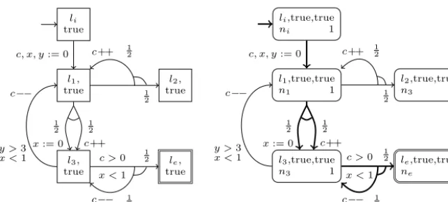
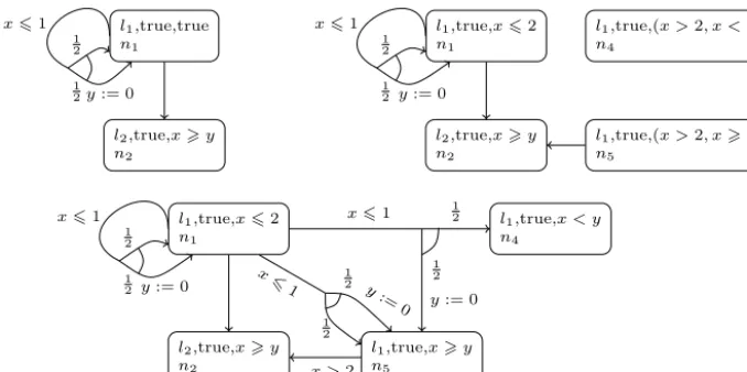
Fig. 1.Left: an example PTPP. Right: initial abstractionAi(P), labelled with node ids and upper probability bounds, and with abstract adversaryσamarked

in bold.

σ

is an adversary ofM

}

. Probabilities from the initial state si of the MDP are denoted by omitting the subscript si, i.e.

pσ_M

=

pσ_M,s

i,p

min

M

=

pminM,si, and p

max M

=

p

max M,si.

2.3. Probabilistic timed programs (PTPs)

The systems we will verify areprobabilistic timed programs(PTPs)[17], which can be thought of as MDPs extended with state variables and real-valued clocks (or as probabilistic timed automata with state variables). For simplicity, we assume that a PTP contains aninitiallocation which must be left immediately and never re-entered, and anerror location which cannot be left. We also make the common assumption that models arestructurally non-Zeno[23].

Definition 2(PTP).A PTP is a tupleP

=

(

L

,

V

,

X

,

li

,

ui

,

le

,

I

,

T

)

where:

•

Lis a finite set oflocationsandli

,

le

∈

Lareinitialanderror locations;

•

V

is a finite set ofstate variablesandui

∈

Val

(

V

)

is theinitial valuation;

•

X

is a finite set ofclocksand

I

:

L

→

Zones

(

X

)

is theinvariant condition, where we assume

I

(

li

)

= {

0

}

;

•

T

:

L

→

P

(

Trans

(

L

,

V

,

X

))

is the probabilistic transition function, where Trans

(

L

,

V

,

X

)

=

Asrt

(

V

)

×

Zones

(

X

)

×

D

(

Assn

(

V

)

×

P

(

X

)

×

L

)

.

A (concrete)stateof a PTP P is a tripleq

=

(

l

,

u

,

v

)

∈

L

×

Val

(

V

)

×

R

X₀ such that v

∈

I

(

l

)

. The set of all states is denoted

Qc

(

P

)

, or Qc ifP is clear from the context. The initial state isqi

=

(

li

,

ui

,

0), and the set of error states is Qe

= {

(

le

,

u

,

v

)

|

v

∈

I

(

le

)

}

. A step of the PTP from state

(

l

,

u

,

v

)

consists of somedelay

δ

0 followed by atransition

(

G

,

E

, )

∈

T

(

l

)

. The transition comprises aguard

G

,enabling condition

E

and probability distribution

=

λ

1

(

f1

,

r1

,

l1

)

+ · · · +

λ

k

(

fk

,

rk

,

lk

)

over triples containing anupdate fj

∈

Assn

(

V

)

,clock resets rj

⊆

X

andtarget location lj

∈

L.

The delay

δ

must be chosen such that the invariant

I

(

l

)

remains continuously satisfied; since

I

(

l

)

is a (convex) zone, this is equivalent to requiring that both vandv

+

δ

satisfy

I

(

l

)

. The chosen transition must beenabled, i.e., the guard

G

and the enabling condition

E

must be satisfied byuandv

+

δ

, respectively. An assignment, set of clocks to reset and successor location are then selected at random, according to the distribution

.

Formally, the semantics of PTP P is given by an MDP

J

P

K

=

(

Qc

,

qi

,

Qe

,

T

)

where

λ

1

(

l1

,

u1

,

v1

)

+ · · · +

λ

k

(

lk

,

uk

,

vk

)

∈

T

(

l

,

u

,

v

)

if and only if there are

δ

0 and

(

G

,

E

, λ

1

(

f1

,

r1

,

l1

)

+ · · · +

λ

k

(

fk

,

rk

,

lk

))

∈

T

(

l

)

such that: (i) u

G

; (ii) v

+

δ

∈

I

(

l

)

∩

E

; (iii)uj

=

fj

(

u

)

for all j; and (iv) vj

=

(

v

+

δ)

[

rj

:=

0

] ∈

I

(

lj

)

for all j. Thus, any adversary

σ

:

Qc+

→

D

(

Qc

)

of

J

P

K

isinducedby two functions

δ

σ

:

Qc+

→

R

0 and

τσ

:

Qc+

→

Trans

(

L

,

V

,

X

)

such that

δ

σ

(

wq

)

and

τσ

(

wq

)

∈

T

(

l

)

satisfy (i)–(iv) for all w

∈

Q_c∗ andq

=

(

l

,

u

,

v

)

.

Our focus in this paper is determining theminimumormaximum probabilityof reaching an error state in PTPP, denoted

pmin_P andpmax_P , respectively. These are defined as the values pmin_JPK andpmax_JPK for its MDP semantics

J

P

K

. We determine the desired value up to a given precision

ε

>

0 by producing lower and upper bounds plb_P,min

pmin_P

pub_P,min or plb_P,max

pmax_P

pub_P,max which differ by at most

ε

.

3. Abstraction refinement for PTPs

We now introduce our abstraction refinement approach for PTPs, which we calllocal abstraction refinement. Our abstrac-tions are based on MDPs and yield both lower and upper bounds on the desired probability. Theouter bound (plb_P,min or

pub_P,max) is obtained from an adversary

σ

a on the abstract MDP (which overapproximates the choices available to concrete adversaries), while theinnerbound (pub_P,minorplb_P,max) is based on a partialconcretisationof

σ

a.

In the next section, we describe the basic ideas underlying our abstractions; in subsequent sections, we describe in more detail how to generate suitably precise abstractions using a refinement loop. Throughout, we will assume a fixed PTP

P

=

(

L

,

V

,

X

,

li

,

ui

,

le

,

I

,

T

)

with semantics

J

P

K

=

(

Qc

,

qi

,

Qe

,

T

)

.

3.1. MDP abstractions

The abstraction for a PTP P in our approach is an MDP, which, for convenience, we augment with concretisation infor-mation.

Definition 3 (MDP abstraction). For a probabilistic timed program P, an abstract state (or node) is a triple n

=

(

l

,

ϕ

,

ρ

)

∈

L

×

Asrt

(

V

)

×

Zones

(

X

)

. We useQa

(

P

)

to denote the set of all abstract states. AnMDP abstractionis a tuple A

=

(

N

,

ni

,

Ne

,

T

)

, where:

•

N

⊆

Qa

(

P

)

is a finite set of nodes,ni

∈

N is the initial node, andNe

⊆

N the set of error nodes;

•

T

:

N

→

P

(

Trans

(

N

,

V

,

X

))

maps nodes to finite sets of abstract transitionsin Trans

(

N

,

V

,

X

)

=

Asrt

(

V

)

×

Zones

(

X

)

×

D

(

Assn

(

V

)

×

P

(

X

)

×

N

)

.

The set ofdead nodesfrom whichNe is not reachable is denoted byNd.

In order to formalise the relationship between an MDP abstraction A and its corresponding PTP P, we introduce the notion of reflections. Recall from the definition of

J

P

K

that any adversary

σ

is induced by functions

δ

σ

:

Qc+

→

R

0 and

τ

σ

:

Qc+

→

T

, such that, for wq

∈

Qc+ with q

=

(

l

,

u

,

v

)

and

τ

σ

(

wq

)

=

(

G

,

E

, λ

1

(

f1

,

r1

,

l1

)

+ · · · +

λ

k

(

fk

,

rk

,

lk

))

, we get

σ

(

wq

)

=

λ

1q1

+ · · · +

λ

kqk withqj

=

(

lj

,

fj

(

u

), (

v

+

δ

σ

(

wq

))

[

rj

:=

0

]

)

. A reflection captures the idea that every concrete adversary can be simulated in an abstraction; if, in addition, every transition in the abstraction represents a special case of a concrete transition, we call this abstractionsound.

Definition 4 (Reflection). Let A

=

(

N

,

ni

,

Ne

,

T

)

be an MDP abstraction for P. A reflection of adversaries for A is a map

∇

:

Qc+

×

R

0

→

N with the following properties:

•

∇

(

wq

, δ)

=

niiffq

=

(

li

,

_

,

_

)

and

∇

(

wq

, δ)

∈

Ne iffq

∈

Qe;

•

for any adversary

σ

of

J

P

K

, let

∇

σ

:

Qc+

→

N be thereflection of

σ

, defined as

∇

σ

(

w

)

=

∇

(

w

, δ

σ

(

w

))

.

Then for any path w

∈

Q_c+, where

σ

(

w

)

=

λ

1q1

+ · · · +

λ

kqk is induced by

δ

σ

(

w

)

and

τσ

(

w

)

=

(

G

,

E

, λ

1

(

f1

,

r1

,

l1

)

+

· · · +

λ

k

(

fk

,

rk

,

lk

))

, there are

G

,

E

such that the set T

(

∇

σ

(

w

))

contains an abstract transition of the form

(

G

,

E

, λ

1

(

f1

,

r1

,

∇

σ

(

wq1

))

+ · · · +

λ

k

(

fk

,

rk

,

∇

σ

(

wqk

)))

.

The need to have a delay as an extra argument arises from the behaviour of refinement with respect to clock constraints (see Section 3.4). The delay is effectively a prophecy variable [1] representing the next decision of the adversary. This dependency means, in particular, that we do not have a straightforward simulation relation between concrete and abstract states; the reflection allows us, however, to construct a simulation for each concrete adversary (seeTheorem 1).

Definition 5 (Concretisable transitions). Let A

=

(

N

,

ni

,

Ne

,

T

)

be an MDP abstraction for P. A hasconcretisable transitions if, for each noden

=

(

l

,

ϕ

,

ρ

)

∈

N and abstract transition

τ

=

(

G

,

E

, λ

1

(

f1

,

r1

,

n1

)

+ · · · +

λ

k

(

fk

,

rk

,

nk

))

∈

T

(

n

)

, wherenj

=

(

lj

,

ϕ

j

,

ρ

j

)

for all j, the PTP P contains a concrete transition

(

G

,

E

, λ

1

(

f1

,

r1

,

l1

)

+ · · · +

λ

k

(

fk

,

rk

,

lk

))

∈

T

(

l

)

with

G

⇒

G

and

E

⊆

E

.

Definition 6 (Sound abstraction). An MDP abstraction A for PTP P is sound if it has a reflection of its adversaries and concretisable transitions.

All our abstractions will be sound and have the following additional property.

Definition 7 (Tight abstraction). An MDP abstraction A is tight if, for every abstract transition

(

G

,

E

, λ

1

(

f1

,

r1

,

n1

)

+ · · · +

The significance of these properties is as follows. Soundness allows us to obtain correct bounds, while tightness ensures progress. Specifically, a reflection of adversaries ensures that the reachability probabilities in the MDP underlying A yield correctouter bounds plb_P,min

:=

pmin_A and pub_P,max

:=

pmax_A (see Theorem 1) while concretisability of transitions means that we obtain correctinnerbounds by partially concretising an abstract adversary (seeTheorem 3). Tightness ensures that each refinement step is aproperrefinement, in the sense that each node obtained by splitting a nodeneither satisfies stronger constraints thannor has stronger enabledness conditions on its outgoing transitions (seeTheorems 4 and 5).

Theorem 1.If A is a sound MDP abstraction for PTP P , then pmin

A

pminP and p max

A

p

max P .

Proof. Let A

=

(

N

,

ni

,

ne

,

T

)

be an MDP abstraction for P with a reflection of adversaries

∇

:

Qc+

×

R

0

→

N, and let

σ

be an arbitrary adversary of

J

P

K

. Consider the MDP M

=

(

Q_c+

,

qi

,

{

wq

∈

Qc+

|

q

∈

Qe

}

,

T

)

with the singleton transition sets

T

(

w

)

= {

λ

1

(

wq1

)

+ · · · +

λ

k

(

wqk

)

}

obtained from

σ

(

w

)

=

λ

1q1

+ · · · +

λ

kqk for allw. This is essentially the DTMC induced by

J

P

K

and

σ

, and satisfies pmin

M

=

pmaxM

=

pσJPK.

By the assumption that li cannot be revisited, all reachable states of M lie inqiQr∗, where Qr

=

(

L

\ {

li

}

)

×

Val

(

V

)

×

R

X

0. Consider the relation R

:= {

(

wq

,

∇

σ

(

q

))

|

wq

∈

qiQr∗

}

. From the definition of

∇

, we have that, for all

(

w

,

n

)

∈

R,

w

=

qi iff n

=

ni, w

∈

Qe iff n

∈

Ne, and T

(

∇

σ

(

w

))

contains an abstract transition

(

G

,

E

, λ

1

(

f1

,

r1

,

∇

σ

(

wq1

))

+ · · · +

λ

k

(

fk

,

rk

,

∇

σ

(

wqk

)))

corresponding to the sole transition

λ

1

(

wq1

)

+ · · · +

λ

k

(

wqk

)

in T

(

w

)

, such that

(

wqj

,

∇

σ

(

wqj

))

∈

R for all j. Thus, R is a probabilistic simulation, and we get pmin

A

pminM

pσJPK and p max

A

pmaxM

pσJPK [6]. Since the argument works for arbitrary

σ

, we also get pmin_A

pmin_JPK

=

pmin_P andpmax_A

pmax_JPK

=

pmax_P .

2

To build abstractions for PTPs, we start with aninitial abstraction, which is defined as follows.

Definition 8(Initial abstraction).For a locationlof PTP P, letnl denote the abstract state

(

l

,

true

,

I

(

l

))

. Theinitial abstraction forP is the MDP abstraction Ai

(

P

)

:=

(

{

nl

|

l

∈

L

}

,

nli

,

{

nle

}

,

T

)

where: T

(

nl

)

= {

α

l

(

τ

)

|

τ

∈

T

(

l

)

}

and

α

l

(

G

,

E

, λ

1

(

f1

,

r1

,

l1

)

+

· · · +

λ

k

(

fk

,

rk

,

lk

))

=

(

G

,

E

, λ

1

(

f1

,

r1

,

nl1

)

+ · · · +

λ

k

(

fk

,

rk

,

nlk

))

with

E

=

I

(

l

)

∩

E

∩

j

[

rj

:=

0

]

I

(

lj

)

. Theorem 2.The initial abstraction Ai

(

P

)

for PTP P is sound and tight.

Proof. Let Ai

(

P

)

=

(

{

nl

|

l

∈

L

}

,

nli

,

{

nle

}

,

T

)

. We define

∇

:

Qc+

×

R

0

→

N by

∇

(

wq

, δ)

=

nl forq

=

(

l

,

v

,

t

)

. Clearly,

∇

maps

(

wq

, δ)

tonli iffl

=

li, and tonle iffq

∈

Qe. Let

σ

be an adversary of

J

P

K

induced by the delays

δ

σ

(

q

)

and transitions

τσ

(

q

)

as defined inDefinition 4. Then, for each w

∈

Qc∗ andq

=

(

l

,

v

,

t

)

,

∇

σ

(

wq

)

=

nl and, by the definition of Ai

(

P

)

,T

(

nl

)

contains the abstract transition

α

l

(

τσ

(

wq

))

=

(

G

,

E

, λ

1

(

f1

,

r1

,

nl1

)

+ · · · +

λ

k

(

fk

,

rk

,

nlk

))

for

τσ

(

wq

)

=

(

G

,

E

, λ

1

(

f1

,

r1

,

l1

)

+

· · · +

λ

k

(

fk

,

rk

,

lk

))

. Altogether, this means that

∇

is a reflection of adversaries and, since concretisability of transitions is ensured by the obvious mapping of

α

l

(

τ

)

to

τ

, the initial abstractionAi

(

P

)

is sound.

Tightness is achieved by using the strengthened enabledness condition

E

in

α

l

(

τ

)

(since all state assertions are true,

G

does not need to be changed).

2

To extract the complementary (inner) bound pub_P,minorplb_P,max from an MDP abstractionA, we will need the notion of a (memoryless)abstract adversary, which selects an outgoing transition from each nodenof A. In practice, we obtain such an adversary when computing the extremal reachability probabilities pmin_A,n orpmax_A,n for each nodenin A.

Definition 9 (Abstract adversary). An abstract adversary for an MDP abstraction A

=

(

N

,

ni

,

Ne

,

T

)

is a function

σ

a

:

N

→

Trans

(

N

,

V

,

X

)

such that

σ

a

(

n

)

∈

T

(

n

)

for alln

∈

N.

Example 2.Fig. 1(right) shows the initial MDP abstraction Ai

(

P

)

for PTPP fromExample 1(Fig. 1, left), for which we want to determine the maximum error probability. The top of each box shows the abstract state (node); underneath is (to the left) a node id and (to the right) the computed maximum probability of reaching error nodene. A corresponding adversary

σ

ais indicated in bold.

An abstract adversary resolves the nondeterminism in the MDP, giving a discrete-time Markov chain which will allow us to compute pub_P,min or plb_P,max. More precisely, we build a (partial)concretisation, based on a forward exploration through the model. We explore the Markov chain induced by

σ

a usingdiscrete states s

=

(

n

,

u

)

consisting of a noden

=

(

l

,

ϕ

,

ρ

)

of A and a valuation uwithu

ϕ

. Interleaved with these forward exploration steps, we perform backwards propagation oftime constraints, starting with the invariants of the newly expanded successor states, which are then iteratively strengthened. We formalise this as follows.

•

a set S

⊆

N

×

Val

(

V

)

of discrete statess

=

(

n

,

u

)

, with a subset O

⊆

S ofopenstates whose successors still have to be explored;

•

a set E ofedges e

=

(

s

, λ,

r

,

s

)

, representing edges of the adversary transitions, with the associated probability

λ

and resetsr. For a state s

=

(

n

,

u

)

,Es

⊆

E is the set of edges with sources. We have:

– Es

= ∅

ifs

∈

O orn

∈

Nd

∪

Ne is a dead or error node;

– otherwise, Es

= {

(

s

, λ

j

,

rj

, (

nj

,

fj

(

u

)))

|

1

j

k

}

based on the edges in

σ

a

(

n

)

=

(

G

,

E

, λ

1

(

f1

,

r1

,

n1

)

+ · · · +

λ

k

(

fk

,

rk

,

nk

))

.

We denote by S

= {

s

∈

S

|

Es

= ∅}

the set ofexpandedstates inC.

Every partial concretisation induces time constraints

η

:

(

S

∪

E

)

→

Zones

(

X

)

and bounds

π0

,

π1

:

S

→ [

0

,

1

]

on reachability probabilities as follows.

•

Let the zones

η

(

s

),

η

(

e

)

for statessand edgesebe the greatest solutions to the fixpoint equations: – for alls

=

(

n

,

u

)

withn

=

(

l

,

ϕ

,

ρ

)

:

η

(

s

)

=

ρ

∩

(

ρ

∩

_e∈Es

η

(

e

))

,

– for eache

=

(

s

, λ,

r

,

s

)

withs

=

(

n

,

u

),

σ

a

(

n

)

=

(

G

,

E

, )

:

η

(

e

)

=

E

∩ [

r

:=

0

]

η

(

s

)

.

•

The probability bounds

π

b

(

s

)

forb

∈ {

0

,

1

}

are the least solutions to:

–

π

b

(

n

,

u

)

=

1 forn

∈

Ne an error node, –

π

b

(

n

,

u

)

=

0 forn

∈

Nda dead node, –

π

b

(

s

)

=

b fors

∈

O, and

–

π

b

(

s

)

=

(s,λ,r,s)∈E

λ

·

π

b

(

s

)

otherwise (i.e. fors

∈

S).

The idea of this construction is that a partial concretisation whose associated time constraints are satisfiable represents a portion of the model on which the abstract adversary’s chosen transitions can be consistently followed by a concrete adversary;

π0

(

ni

,

ui

)

and

π1

(

ni

,

ui

)

then give a lower bound and an upper bound onpσP for any adversary

σ

doing so.

We can therefore use the probability bounds

π

bfrom the concretisation of a maximising or minimising abstract adversary to determine inner bounds, i.e., we takeplb_P,max

:=

π0

(

ni

,

ui

)

orpubP,min

:=

π1

(

ni

,

ui

)

.

In order to formalise this, we first define some auxiliary sets capturing the relationship between concrete and discrete states. Fors

=

(

n

,

u

)

∈

S, withn

=

(

l

,

ϕ

,

ρ

)

, we let Qs

= {

(

l

,

u

,

v

)

∈

Qc

(

P

)

|

v

∈

η

(

s

)

}

and define QS

=

s∈SQs and QS

=

s∈SQs; forq

∈

Qc

(

P

)

,Sq

= {

s

∈

S

|

q

∈

Qs

}

andSq

= {

s

∈

S

|

q

∈

Qs

}

.

We then say that a concrete adversary

σ

for P follows the partial concretisation C

=

(

S

,

O

,

E

)

if there is a map

s

:

Q+_S

→

S such that, for each path w

=

w1

. . .

wm

∈

Q+_S, if wm

∈

Q_S and

σ

(

w

)

=

λ

1q1

+ · · · +

λ

kqk, then Es(w)

=

{

(

s

(

w

), λ

j

,

rj

,

s

(

wqj

))

|

1

j

k

}

for somer1

, . . . ,

rk

⊆

X

.

Theorem 3.Let C

=

(

S

,

O

,

E

)

be a partial concretisation for adversary

σ

aof A, such that all zones

η

(

s

)

for s

∈

S and

η

(

e

)

for e

∈

E

are non-empty. Then:

1. there exists a concrete adversary

σ

following C; 2. for any such

σ

, we have

π0

(

ni

,

ui

)

pσP

π1

(

ni

,

ui

)

.

Proof. 1. Let w

=

w1

. . .

wm

∈

Q_S+ with wm

=

(

l

,

u

,

v

)

. Let s

(

w

)

be

(

n

,

u

)

∈

Swm withn

=

(

l

,

ϕ

,

ρ

)

(chosen arbitrarily if

|

w

| =

1) and let the abstract adversary’s chosen transition be

σ

a

(

n

)

=

(

G

,

E

, λ

1

(

f1

,

r1

,

n1

)

+ · · · +

λ

k

(

fk

,

rk

,

nk

))

, wherenj

=

(

lj

,

ϕ

j

,

ρ

j

)

. Sinces

(

w

)

∈

Swm, we have thatv

∈

η

(

s

(

w

))

=

ρ

∩

(

ρ

∩

e∈Es(w)

η

(

e

))

. Therefore, there exists some

δ

∈

R

0

such that v

+

δ

∈

ρ

∩

_e∈Es(w)

η

(

e

)

(andv

+

∈

ρ

for all 0

δ

, since

ρ

is convex).

By concretisability of transitions, there is a corresponding concrete transition

τ

=

(

G

,

E

, λ

1

(

f1

,

r1

,

l1

)

+ · · · +

λ

k

(

fk

,

rk

,

lk

))

with

G

⇒

G

and

E

⊆

E

. Due to the above, a concrete adversary can choose this concrete transition after a suitable delay

δ

, getting the distribution

λ

1q1

+ · · · +

λ

kqk, whereqj

=

(

lj

,

fj

(

u

),

vj

)

withvj

=

(

v

+

δ)

[

rj

:=

0

]

. The edges in Es are ej

=

(

s

(

w

), λ

j

,

rj

,

sj

)

, where sj

=

(

nj

,

fj

(

u

))

; since

δ

was chosen such that v

+

δ

∈

η

(

ej

)

=

E

∩ [

rj

:=

0

]

η

(

sj

)

for all j, we get vj

∈

η

(

sj

)

, and thus sj

∈

Sqj, so we can choose s

(

wqj

)

=

sj. Iterating this argument, we get a concrete adversary followingC.

2. Let

σ

be a concrete adversary following C, w

=

w1

. . .

wm be any path within QS in the Markov chain induced by P and

σ

, and s1

, . . . ,

sm be the corresponding path in the Markov chain

(

S

,

TS

)

represented by C (with transitions

T

(

s

)

=

λ

1s1

+ · · · +

λ

kskforEs

= {

(

s

, λ

j

,

rj

,

sj

)

|

1

j

k

}

). By the above correspondence, the paths have equal probabilities. From the soundness of the abstraction, we get a correspondence regarding reachability of the error:

•

sm

=

(

n

,

u

)

is an error state (n

∈

Ne) iffqmis an error state (qm

∈

Qe);

•

ifsm

=

(

n

,

u

)

withn

∈

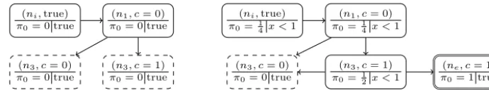
Nd, i.e.Ne is not reachable fromn, then Qe is likewise not reachable fromqm;

[image:8.561.102.447.56.120.2]

Fig. 2.Two partial concretisations for the MDP abstraction ofFig. 1.

This implies that the reachability probabilities of Se

= {

(

n

,

u

)

∈

S

|

n

∈

Ne

}

and of Se

∪

O are a lower and an upper bound on pσ_P, and (see e.g. Thm. 1.3.2 in[22]) they are exactly the least solutions of:

•

p

(

s

)

=

1 ifs

∈

Se (resp.s

∈

Se

∪

O), and

•

p

(

s

)

=

T

(

s

)(

s

)

p

(

s

)

otherwise,

making them equal to

π0

and

π1

.

2

Example 3. We return to the MDP abstraction and abstract adversary

σ

a of Example 2, shown in Fig. 1 (right). Fig. 2 (left) shows a partial concretisation. The top of each box shows the discrete state; the bottom shows the lower probability bound

π0

(since we are computing maximum probabilities) and time constraint

η

(

s

)

. Unexpanded states are drawn with dashed lines. For clarity, edge details are omitted.Fig. 2(right) shows a subsequent partial concretisation, expanding state

(

n3

,

c

=

1

)

. The outgoing transition contains a time constraint x

<

1, which gets propagated backwards. One successor is error state

(

ne

,

c

=

1

)

, leading to an increase in the lower bounds.

3.2. The refinement loop

Our approach to computing reachability probabilities for PTPs is based on an iterative abstraction refinement loop, which generates increasingly precise MDP abstractions. At each iteration, we first compute minimum or maximum reachability probabilities for the MDP, yielding an (outer) bound plb,min_{or p}ub,max _{and an abstract adversary. Then, we partially} con-cretise this adversary, based on a forward exploration through the model, yielding after each step a complementary (inner) probability bound pub,min

=

π1

(

ni

,

ui

)

or plb,max

=

π0

(

ni

,

ui

)

. If the difference between the lower and upper bounds for the initial state of the model falls below a pre-specified tolerance

ε

, then abstraction refinement terminates. Otherwise, concretisation continues until aninconsistencyis identified, which will be used torefinethe abstraction.

There are two classes of inconsistencies which may occur during concretisation:state-basedinconsistencies, which, due to tightness, will always manifest themselves as the failure of a valuation to satisfy the guard of the adversary’s chosen transition, andtime-basedinconsistencies, which occur when there is no consistent choice of delay, and manifest themselves as the occurrence of an empty zone

η

(

_

)

= ∅

in the concretisation. Accordingly, there are two separate refinement operations for an MDP abstraction:state refinement, which splits a node with a predicate

ϕ

∈

Asrt

(

V

)

; andtime refinement, which splits based on an inconsistent set of clock difference constraints c1

, . . . ,

ck. The former is relatively standard, for abstraction refinement techniques; the latter is a novel method that we have developed for the PTP model. In the next two sections, we describe each of these in more detail. The main refinement loop is sketched in Fig. 3. Pseudocode and descriptions of auxiliary functions addState(), expand() and backpropagate() are shown inFigs. 4 and 5. Details of the refinement functions stateRefine() and timeRefine() are given in the next sections. The algorithm maintains an MDP abstractionA

=

(

N

,

ni

,

Ne

,

T

)

, along with:

•

an abstract adversary

σ

aand resulting outer bounds pminA,n orpmaxA,n;

•

a partial concretisation

(

S

,

O

,

E

)

, along with the associated inner bounds

π

b

(

s

)

and time constraints

η

(

s

)

and

η

(

e

)

for all s

∈

S ande

∈

E;

•

a setbp

⊆

S of states whose time constraints still need to be strengthened to satisfy the required fixpoint equations (see p.43).

The outcome of the algorithm, if it terminates, is a set containing an inner and an outer bound

{

π

b

(

ni

,

ui

),

pdir_A,ni

}

. Note that termination cannot be guaranteed in general, since the class of PTPs is Turing complete (it contains counter automata as a subclass). If the system is a PTA, then in the worst case the refinement procedure constructs the region graph, since in each iteration we nontrivially split a clock zone; see the proof ofTheorem 5.

3.3. State refinement

State refinement is triggered when forward exploration encounters a state

(

n

,

u

)

such thatu does not satisfy the guard

Input: PTPP,dir∈ {min,max},ε≥0 A:=Ai(P);

b:=ifdir=minthen1else0; Loop:

computeσaandpdirA,nforn∈N; S,O,E,bp:= ∅;

addState(ni,ui);πb(ni,ui):=b;

while|pdir

A,ni−πb(ni,ui)|>εdo

takes=(n,u)fromO; let(G,E, )=σa(n);

ifuGthenstateRefine(n,u); gotoLoop; expand(s);

ifbackpropagate()thengotoLoop; updateπb;

[image:9.561.189.343.55.195.2]

return{πb(ni,ui),pdirA,ni};

Fig. 3.The refinement loop. In each iteration, the abstract adversary is computed, followed by a partial concretisation. The inner loop uses functions expand(s) to obtain the successors of s and add them to the concretisation, and backpropagate() to ensure consistency of the time constraints. It is aborted if a refinement step occurred.

addState(s) ifs∈/Sthen

let(n,u)=s,

(l,ϕ,ρ)=n; addstoS; η(s):=ρ; ifn∈/Nd∪Ne then

addstoO;

expand(s)

let(n,u)=s,(G,E, )=σa(n);

foreachλj(fj,rj,nj)indo sj:=(nj,fj(u));

addState(sj);

addej:=(s, λj,rj,sj)toE;

η(ej):=E∩ [rj:=0]η(sj);

[image:9.561.127.385.245.315.2]

ifη(s)η(ej)thenaddstobp;

Fig. 4.Procedure addState(s), left, adds a new statesto the partial concretisation, initialises its time constraintsη(s), and schedules it for expansion (puts it inO) if necessary. Procedure expand(s), right, determines the successorss1, . . . ,skofs, adds the edges fromstosj, and addsstobpif its time constraints

now need to be strengthened.

backpropagate() whilebp= ∅do

takesfrombp, wheres=(n,u)andn=(l,ϕ,ρ); η:=RX

0;

foreache∈Esdoη:=η∩η(e);

ifη= ∅then

C:=unsatisfiable core forρ,{η(e)|e∈Es};

timeRefine(n,C); return true; η(s):=ρ∩ η;

foreache=(s, λ,r,s)∈Edo let(n,u)=s,(G_{,E, )=σ(n);}

η(e):=E_{∩ [r:=0]η(s);}

ifη(e)= ∅then

C:=unsatisfiable core forE[r:=0],η(s); timeRefine(n,C); return true;

ifη(s)η(e)thenaddstobp; return false;

Fig. 5.backpropagate() strengthens the constraintsη(_)in order to make them consistent. A statesis inbpifη(s)does not implyη(e)for some edge e=(s, λ,r,s). The function takes states frombpand strengthens their constraints (potentially causing new additions tobp) until a contradiction occurs (in which case a refinement step is triggered and we returntrue) orbpis empty (in which case a fixpoint was reached, and we returnfalse). Since in each iteration one of the finitely many zonesη(s)shrinks, and zones satisfy the descending chain condition, the procedure always terminates.

sense that we only use information directly related to state

(

n

,

u

)

, rather than having to take the entire concretisation into account. The result of this split is a pair of new nodesn₊

=

(

l

,

ϕ

∧

g

,

ρ

)

andn₋

=

(

l

,

ϕ

∧ ¬

g

,

ρ

)

. We then modify the sets of transitions:

•

first,n₊andn₋ both inherit the outgoing transitions inT

(

n

)

;

•

then, for each

τ

=

(

G

,

E

, λ

1

(

f1

,

r1

,

n1

)

+ · · · +

λ

k

(

fk

,

rk

,

nk

))

inA:

– find the indicesI

:= {

j

|

nj

=

n

}

of edges which need to be redirected;

– for each possible redirection

ν

:

I

→ {

n₊

,

n₋

}

, add a new transition

τν

:=

(

G

ν

,

E

, λ

1

(

f1

,

r1

,

n1

)

+ · · · +

λ

k

(

fk

,

rk

,

nk

))

withn_j

=

ν

(

j

)

for j

∈

I,n_j

=

njotherwise, and

G

ν obtained from

G

by adding the corresponding preconditions g

◦

fj or

¬

g

◦

fjfor j

∈

I;

[image:9.561.177.366.364.518.2]