Adaptive Algorithms for Sparse
Nonlinear Channel Estimation
The Harvard community has made this
article openly available.
Please share
how
this access benefits you. Your story matters
Citation
Kalouptsidis, Nicholas, Gerasimos Mileounis, Behtash Babadi,
and Vahid Tarokh. 2009. Adaptive algorithms for sparse nonlinear
channel estimation. Paper presented at the 2009 IEEE Workshop on
Statistical Signal Processing, Cardiff, Wales, UK.
Citable link
http://nrs.harvard.edu/urn-3:HUL.InstRepos:4481494
Terms of Use
This article was downloaded from Harvard University’s DASH
ADAPTIVE ALGORITHMS FOR SPARSE NONLINEAR CHANNEL ESTIMATION
Nicholas Kalouptsidis
#, Gerasimos Mileounis
#, Behtash Babadi
∗and Vahid Tarokh
∗#
Dept. of Informatics and Telecommunications, University of Athens, Ilisia 15784, Greece
∗
School of Engineering and Applied Sciences, Harvard University, Cambridge, MA 02138
:
{
kalou,gmil
}
@
di.uoa.gr
,
{
behtash,vahid
}
@
seas.harvard.edu
ABSTRACT
In this paper, we consider the estimation of sparse nonlinear communication channels. Transmission over the channels is represented by sparse Volterra models that incorporate the ef-fect of Power Amplifiers. Channel estimation is performed by compressive sensing methods. Efficient algorithms are pro-posed based on Kalman filtering and Expectation Maximiza-tion. Simulation studies confirm that the proposed algorithms achieve significant performance gains in comparison to the conventional non-sparse methods.
Index Terms— Volterra series, Adaptive estimation, Com-pressive sensing, Kalman filtering, Expectation Maximiza-tion.
I. INTRODUCTION
Channel nonlinearities are mainly due to Power Amplifiers (PA). PAs located at an access point of a downlink channel (base stations in cellular systems and repeaters for satellite links) often operate close to saturation in order to achieve power efficiency. The models employed in the description of PAs are either static (memoryless) or dynamic (models with memory).
Wireless communication channels are characterized by time varying multipath propagation effects. Quite often in prac-tice, several reflections reach the receiver at different time in-stances. These reflections arrive at the receiver with longer delay than the first group. Hence, the wireless channel is modeled by sparse fading rays and long zero samples and thus admits a sparse representation [1]. The sparseness char-acteristic is preserved when the PA representation is also de-scribed by a sparse model [2]. Recent experimental results reported in [2] indicate better performance if sparse nonlinear models are employed for the representation of PA. Moreover, the time-varying nature of the wireless channels suggest the use of adaptive algorithms that minimize transmission delays and take advantage of parameters sparsity. Thus, compressive sensing provides a promising framework for such develop-ments. Adaptive algorithms for sparse channel estimation are developed in [3, 4]. In [3] two different sparsity constraints are incorporated into the quadratic cost function of the LMS algorithm, to take into account the sparse channel coefficient vector. An`1-regularized RLS type algorithm based on a low
complexity Expectation-Maximization, is derived in [4]. In this paper we focus on adaptive estimation of sparse nonlinear communication channels. Adaptation is carried out
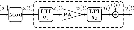
{si} x(t)
Mod LTI
g1
z(t)
PA w(t)
LTI
g2
r(t) +
v(t)
y(t)
Fig. 1. Digital satellite link
by recursive algorithms that combine Expectation Maximiza-tion and Kalman filtering. The expectaMaximiza-tion step is carried out by Kalman filtering while the maximization step corresponds to a soft-thresholding function due to the`1regularization.
The rest of the paper is organized as follows. Nonlin-ear channels and sparse channel estimation are discussed in Section II. The proposed algorithms for adaptive tracking of sparse nonlinear channels are given in section III. Simulation results are presented in Section IV. Conclusions are discussed in Section V.
II. SPARSE NONLINEAR CHANNEL ESTIMATION
In what follows, power amplifier nonlinear models are in-corporated into the study of two important channels: 1) the satellite link, and 2) the multi-path wireless channel. In both cases, the overall communication channel is represented by baseband Volterra series.
A. Nonlinear channel models
In satellite digital transmission, both the earth station and the satellite repeater employ power amplifiers. The satellite am-plifier operates near saturation due to limited power resources and hence behaves in a nonlinear fashion. The satellite link is represented by the block diagram of Fig. 1. The LTI filter with impulse responseg1describes the cascade of all linear
operations preceding the power amplifier. Likewise the LTI filterg2represents the cascade of all linear devices following the nonlinearity.
An analysis of the above system for static power ampli-fiers is provided by Benedetto and Biglieri [5]. Let us next consider power amplifiers with memory described by Volterra models. To reduce the computational complexity we shall follow standard practice [2, 6] and confine our study to diag-onal Volterra models1. Straightforward calculation lead to the
[image:2.595.326.549.211.261.2]baseband Volterra model
r(t) =
bP−1 2 c X
p=0 Z
· · ·
Z
h2p+1(τ1:2p+1) (1)
×
pY+1
i=1
x(t−τi)
2Yp+1
j=p+2
x∗(t−τ
j)dτ1:2p+1.
whereh2p+1(τ1:2p+1)denotes the baseband kernel with
τ1:2p+1= (τ1, . . . , τ2p+1).
In most cases the filterg1performs a specific functional-ity (for instance pulse shaping) and hence is known. Since in this paper we shall deal with channel estimation using known inputs, we may with no loss of generality assume the input signal is the output of g1. In this case the Volterra
repre-sentation from signalx(t)to signalr(t)gets simpler. More precisely we have
r(t) =
bP−1 2 c X
p=0 Z
h2p+1(t, τ1)|x(t−τ1)|2px(t−τ1)dτ1. (2)
The above expression represents also the multipath chan-nel. In this case the modulated signal is amplified by a power amplifier and then transmitted through the wireless medium. The received waveform is the superposition of weighted and delayed versions of the signal resulting from various multi-paths plus additive white Gaussian noise. We shall assume that the different nonzero fading rays arrive at the receiver at different time instances and they vary slowly with time and frequency hence the wireless channel becomes a frequency selective channel [1] and is described by an impulse response of the form
g2(ρ) =
N X
i=1
aiδ(ρ−τi) (3)
whereN is the number of paths,ai is the attenuation along
pathiandτiis the clustered delay.
B. Sparse channel estimation
The transmission systems described in the previous section operate in continuous time. Discrete Volterra forms result when the modulation at the transmitter and the sampling de-vice at the receiver are taken into account. We shall consider memoryless modulation schemes whereby
x(t) =X
i
siδ(t−iTs). (4)
The sequencesi consists of i.i.d (discrete) complex valued
random variables andTsdenotes the symbol period.
Substi-tutingx(t)from Eq. (4) into (1) yields the discrete baseband Volterra model [5] which can be expressed as a linear regres-sion. Let us define the vector
xi,M2p+1= £
si, si−1,· · ·, si−M2p+1 ¤T
and thei-fold Kronecker product
x(i,Mp+1,p)
2p+1= [⊗ p+1
j=1xi,M2p+1]⊗[⊗ p
k=1x∗i,M2p+1].
The Kronecker product contains all2p+ 1order products of the input withpconjugate copies. The output can be written in the linear regression form
yi= h
xTi,M1· · ·x (p+1,p)T i,M2p+1
i
h1
.. .
h2p+1
+vi (5)
with1≤i≤n. If we stacknsuccessive samples in a column format we obtain
yn=Xnh+vn (6)
whereyn = [y1,· · ·, yn]T,vn = [v1,· · ·, vn]T andXn = £
xT
1,· · ·,xTn ¤T
.
Eq. (6) provides a noisy representation of a block of re-ceived successive samples in terms of the columns of Xn
(also referred to as dictionary), that are formed by the prod-ucts of shifted symbol sequences. The above representation is sparse and hence recovery of the vectorhcan be accom-plished by compressed sensing methods. Next we consider sparsity. It is well documented in the literature that parsi-monious models are highly desirable in the representation of memory PA. In fact it has been experimentally observed [2] that sparse diagonal Volterra models provide enhanced perfor-mance in comparison to the full model. Furthermore, a phys-ical justification of sparsity for the multipath channel is given in [1]. The sparsity of the2p+ 1kernel is at mostsk×sm,
wheresk is the sparsity of the PA andsmis the sparsity of
the multipath coefficients. Similar observations hold for the satellite channel. It thus follows that the vectorhin Eq. (6) is sparse.
Recovery of the locations, the magnitudes and the non-linear coefficients ofhcan be accomplished by the convex program
min
h
½ 1
2kyn−Xnhk 2
`2+γkhk`1 ¾
. (7)
The `1-norm provides a convex relaxation to the `0
quasi-norm. The scalar parameterγ provides a trade-off between sparsity and total squared error. The optimization problem (7) has been widely studied from the perspective of compressive sensing (see, for instance, [7]).
III. ADAPTIVE ALGORITHMS
Since the parameter vector hchanges with time we need a model that captures the corresponding dynamics. A popular technique in the adaptive filtering literature is to describe pa-rameter variation by the first-order model [8]
hn=hn−1+qn,Λ0 =h0+ n X
i=1
qi,Λ0; h0∼ N(h0, σ20IΛ0).
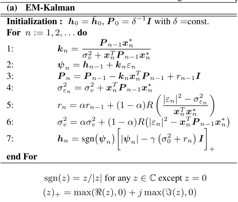
Table 1. Algorithms for sparse nonlinear channel identification
(a) EM-Kalman
Initialization : h0= ¯h0,P0=δ−1Iwithδ=const.
For n:= 1,2, . . .do
1: kn= Pn−1x
∗
n
σ2
v+xTnPn−1x∗n
2: ψn=hn−1+knεn
3: Pn=Pn−1−knxTnPn−1+rn−1I
4: σ2
εn=σ
2
v+xTnPn−1x∗n
5: rn=αrn−1+ (1−α)R
µ
|εn|2−σ2εn
xT
nx∗n
6: σ2
v=ασ2v+ (1−α)R
¡
|εn|2−xTnPn−1x∗n
¢
7: hn=sgn
¡ ψn¢
·
|ψn| −γ¡σ2 0+rn
¢ I
¸
+
end For
sgn(z) =z/|z|for anyz∈Cexceptz= 0 (z)+= max(<(z),0) +jmax(=(z),0)
(b) EM-RLS
Initialization : h0= 0,P0=δ−1Iwithδ=const.
For n:= 1,2, . . .do
1: kn= Pn−1x
∗
n
λ+xT
nPn−1x∗n
2: ψn=hn−1+knεn
3: Pn=λ−1Pn−1−λ−1knxTnPn−1
4: Rn= (1−λ)Pn
5: hn=sgn
¡
ψn
¢£
|ψn| −γ
¡
σ2
0+ diagRn
¢ ¤
+
end For (c) EM-LMS
Initialization : h0= 0,0< µ <2λ−max1
For n:= 1,2, . . .do
1a: hn=hn−1−γsgnhn−1+µx∗nεn
1b: hn=hn−1−γ sgnhn−1
1 +²|hn−1|+µx
∗
nεn
end For
Λ0denotes the support set ofh0, i.e. the set of the non-zero
coefficients. The noise termqnis zero outsideΛ0and
zero-mean Gaussian inside Λ0 with diagonal covariance matrix
Rn,Λ0 = diag[σq21(n), . . . , σ 2
qd(n)], wheredis the`0 norm
ofh0. The variances{σ2qi(n)}
d
i=1 are in general allowed to
vary with time. The stochastic processesv,qand the random variableh0are mutually independent.
We next incorporate Eq. (8) and the convex program (7) into the Expectation-Maximization (EM) framework. The re-sulting adaptive algorithms employ only one iteration per time update for computational purposes. Letθ= ¯h0be the vector
of unknown parameters. Note that under the Gaussian as-sumption postulated above, minimization of (8) is equivalent to the maximization of the log-likelihoodp(yn|θ)augmented by an`1penalty.
To apply the Expectation-Maximization method we have to specify the complete and incomplete data. The vectorhnat
timenis taken to represent the complete data vector, whereas
yn−1 accounts for the incomplete data [9]. In this context
the conditional densityp(hn|yn−1)plays a major role. This
density is Gaussian with mean and covariance:
ψn=E[hn|yn−1]
Pn=E[(hn−ψn)(hn−ψn)H] =σ02I+
n X
t=1 diag[σ2
qi(t)].
Under broad conditions the maximizer of the incomplete likelihood is obtained by maximizing the complete likelihood function through successive application of the following two steps:
E-step :computes the conditional expectation
Q(θ,θbn−1) =Ep(hn|y
n−1;θbn−1)[logp(hn;θ)] (9) M-step : maximizes the Q-function minus the `1-penalty
with respect toθ:
b
θn= arg max
θ
n
Q(θ,bθn−1)−γkθk`1 o
. (10)
Note that
logp(hn;θ) =const.−1
2(hn−ψ(θ))
H
P−n1(hn−ψ(θ)).
Therefore theQ-function takes the form
Q(θ,bθn−1) =const.+θP−n1ψn−
1 2θ
HP−1
n θ (11)
where the constant incorporates all terms that do no involveθ
and hence do not affect the maximization.
The parameterψnis recursively computed by the Kalman
filter [8], see Table 1(a) steps1−3, which in the special case of the time-varying random walk model Eq. (8) takes an RLS type appearance. Note thatεn, in Table 1, denotes the
predic-tion error given byεn=yn−xTnhn−1.
Maximization of theQfunction leads to thesoft thresh-oldingfunction
b
hn,i= sgn
¡ ψn,i
¢"
|ψn,i| −γ
Ã
σ02+
n
X
t=1
σq2i(t)
! #
+ (12)
This operation shrinks coefficients above the threshold in mag-nitude value.
EM-Kalman filter. The Kalman filter computeshbn
un-der the assumption that the variancesσ2
v and{σq2i(n)}
d i are
known. The noise variances can be estimated in various ways. One method is to use the Maximum Likelihood estimates. These estimates can be obtained by maximizing theQ-function.
Alternatively, under the assumption that the state noise is
Rn,Λ0 =rnI, then both noise disturbances can be estimated
adaptively. A smoothed estimate of the state and observation noise can be respectively obtained according to steps 5 and 6 of Table 1(a), whereαis a smoothing parameter andR(x)
is the ramp function (R(x) =xifx ≥ 0and0 otherwise). These two methods for online estimation of the noise distur-bances is due to Jazwinski [10].
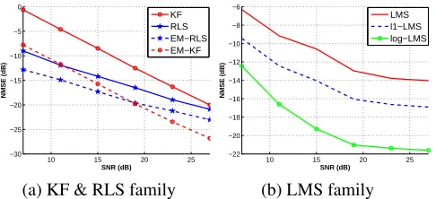
10 15 20 25 −30
−25 −20 −15 −10 −5 0
SNR (dB)
NMSE (dB)
KF RLS EM−RLS EM−KF
(a) KF & RLS family
10 15 20 25
−22 −20 −18 −16 −14 −12 −10 −8 −6
SNR (dB)
NMSE (dB)
LMS l1−LMS log−LMS
(b) LMS family
Fig. 2. NMSE of the three sparse adaptive algorithms
model, Eq. (8), resembles the RLS algorithm. In fact, the RLS can be viewed as a special form of Table 1(a) which pro-vides an alternative for the estimation of the noise variances.
The RLS filter is given by steps 1-3 of Table 1(b) [8], with
σ2
v =λ, Rn= (1−λ)Pn.
Sparse LMS filter. For the purposes of simulations pre-sented in the next section we discuss the LMS variant de-veloped in [3]. LMS updates some convex cost function of the prediction error signalεn plus an `1 penalty. The
up-date equation which minimizes the cost function is given in step 1a of Table 1(c). The authors in [3] replace the`1-norm
penalty by the log-sum penalty function. Hence, the result-ing update equation for this cost function becomes step 1b of Table 1(c). The log-sum penalty function has the potential of being more-sparsity encouraging since it better approximates the non-convex`0-norm.
IV. SIMULATIONS
Experiments were conducted on the multipath channel setup of Eq. (2). The algorithms were run for2000iterations and averaged over50Monte Carlo runs to reduce realization de-pendency. In all experiments the output sequence is disturbed by additive white Gaussian noise for various SNR levels rang-ing from7 to 27dB. The Normalized Mean Square Error, defined as NMSE= 10 log10
³
E[khˆ−hk2
`2]/E[khk 2
`2] ´
, was used to assess performance. The NMSE is computed after500
iterations so that all algorithms have secured convergence. A third order channel model was used to test the derived algorithms. The wireless channel taps for the linear and cu-bic part were generated by sparse Rayleigh fading rays. All rays are assumed to fade at the same Doppler frequency of
fD = 80Hzwith sampling periodTs = 0.8µs. The linear
and the cubic part have equal memory sizeM1 =M3 = 50
and the support signal consists of 2 randomly selected ele-ments for each part. The input signal is drawn from a com-plex Gaussian distributionCN(0,1/4). We observe that the EM-Kalman and EM-RLS algorithms provide gains of7dB
and5dB respectively, over the corresponding conventional non-sparse algorithms.
[image:5.595.59.302.76.187.2]The choice of the parametersγ,λthat were used to com-pare performance of the sparse algorithms are summarized in Table 2 for various SNR levels. The additional parameters re-quired for the LMS are set toµ= 5×10⁻²and²= 10. For
Table 2. Choice of parameters for the sparse algorithms
SNR KF RLS (λ, γ) LMS (`1,log)
7 3×10⁻³ .999,1×10−1 5×10−4,3×10−3
11 2×10⁻³ .999,1×10−1 4×10−4,2×10−3
15 1.4×10⁻³ .997,9×10−2 3×10−4,2×10−3
19 9×10⁻⁴ .995,9×10−2 3×10−4,1.5×10−3
23 6×10⁻⁴ .995,8×10−2 3×10−4,1.5×10−3
27 3.5×10⁻⁴ .991,7×10−2 3×10−4,1.5×10−3
the EM-Kalman and the EM-RLS, the initial noise variance is set toσ2
0= 0.01σx2.
It must be noted that due to the nature of the soft thresh-olding step, the identifiedhnhas many zero entries. This will
allow to implement the EM-Kalman and EM-RLS algorithms in a low-complexity fashion similar to the approach taken in [4]. Thus, the EM-Kalman and EM-RLS algorithms intro-duce complexity gains as well as NMSE performance gains over the non-sparse methods.
V. CONCLUSIONS
In this paper, sparse approximations have been studied for nonlinear channel estimation. Adaptive algorithms combin-ing Expectation-Maximization and Kalman filtercombin-ing were de-veloped and tested by simulations. Significant performance gains were achieved in comparison to the conventional non-sparse methods.
VI. REFERENCES
[1] W.U. Bajwa, J. Haupt, G. Raz, and R. Nowak, “Compressed channel sensing,” inProc. IEEE CISS, 2008, pp. 5–10. [2] H. Ku and J.S. Kenney, “Behavioral modeling of nonlinear rf
power amplifiers considering memory effects,” IEEE Trans. Microw. Theory Tech., vol. 51, no. 12, pp. 2495–2504, Dec. 2003.
[3] Y. Chen, Y. Gu, and A. Hero, “Sparse LMS for system identi-fication,” inProc. IEEE ICASSP, 2009.
[4] B. Babadi, N. Kalouptsidis, and V. Tarokh, “Comparison of spaRLS and RLS algorithms for adaptive filtering,” inProc. IEEE Sarnoff Symposium, 2009.
[5] S. Benedetto and E. Biglieri, Principles of Digital Transmis-sion: with wireless applications, Springer, 1999.
[6] M. Isaksson, D. Wisell, and D. Ronnow, “A comparative analy-sis of behavioral models for RF power amplifiers,”IEEE Trans. Microw. Theory Tech., vol. 54, no. 1, pp. 348–359, Jan. 2006. [7] J.A. Tropp, “Just relax: Convex programming methods for
identifying sparse signals,” IEEE Trans. Inf. Theory, vol. 51, no. 2, pp. 1030–1051, Mar. 2006.
[8] L. Ljung, General structure of adaptive algorithms: Adapta-tion and tracking, in Adaptive System Identification and Signal Processing Algorithms, Eds. N. Kalouptsidis and S. Theodor-idis, 1993.
[9] M. Feder, Statistical Signal Processing Using a Class of Iter-ative Estimation Algorithms, Ph.D. thesis, M.I.T., Cambridge, MA, 1987.
[image:5.595.318.552.91.182.2]