White Rose Research Online URL for this paper:
http://eprints.whiterose.ac.uk/111968/
Version: Accepted Version
Article:
Freeman, Mark C orcid.org/0000-0003-4521-2720 and Groom, Ben (2015) Using equity
premium survey data to estimate future wealth. Review of Quantitative Finance and
Accounting. pp. 665-693. ISSN 0924-865X
https://doi.org/10.1007/s11156-014-0451-7
[email protected] https://eprints.whiterose.ac.uk/ Reuse
Items deposited in White Rose Research Online are protected by copyright, with all rights reserved unless indicated otherwise. They may be downloaded and/or printed for private study, or other acts as permitted by national copyright laws. The publisher or other rights holders may allow further reproduction and re-use of the full text version. This is indicated by the licence information on the White Rose Research Online record for the item.
Takedown
If you consider content in White Rose Research Online to be in breach of UK law, please notify us by
(will be inserted by the editor)
Using equity premium survey data to estimate future wealth
Mark C. Freeman Ben Groom
the date of receipt and acceptance should be inserted later
Abstract We present the …rst systematic methods for combining di¤erent experts’ responses to equity premium surveys. These techniques are based on the observation that the survey data are approximately gamma distributed. This distribution has convenient analytical properties that enable us to address three important problems that investment managers must face. First, we construct probability density functions for the future values of equity index tracker funds. Second, we calculate unbiased and minimum least square error estimators of the future value of these funds. Third, we derive optimal asset allocation weights between equities and the risk-free asset for risk-averse investors. Our analysis allows for both herding and biasedness in expert responses. We show that, unless investors are highly uncertain about expert biases or forecasts are very highly correlated, many investment decisions can be based solely on the mean of the survey data minus any expected bias. We also make recommendations for the design of future equity premium surveys.
Keywords Financial surveys Equity premium Asset allocation Gamma distribution JEL classi…cation G11; G17.
1 Introduction
In recent years a number of surveys have been conducted to solicit informed individuals’ views on the forward looking equity premium. For example Welch (2000, with updates in 2001, 2007 and 2009) and Fernandez and del Campo (2010a) ask economics and …nance professors; Graham and Harvey (2010) is their latest in a series of studies that has taken data from the Global CFO Outlook Survey; whilst Fernandez and del Campo (2010b) take forecasts from analysts and com-panies. This stream of research has generated considerable interest amongst both academics and practitioners. In this paper we present the …rst systematic techniques for optimally combining the con‡icting forecasts of the forward looking equity premium presented in any one of these surveys.
Our methods exploit the observation that estimates of the equity premium are, to good approximation, gamma distributed. This draws in parallels with Weitzman’s (2001) highly in-‡uential use of survey data on the appropriate long term social discount rate for evaluating investments with intergenerational consequences. This distribution has the bene…t of a well de-…ned moment generating function (mgf) and established numerical techniques for determining
the probability density function (pdf) of the population mean conditional on a …nite sample of data.
We use these two features of the gamma distribution to answer questions about the future value of an equity index tracker fund and optimal asset allocation. The fact that a closed-form mgf of the distribution exists allows us to determine unbiased and minimum least square error (MLSE) estimates of the future value, and quantiles of the future value, of the fund. This extends the analysis of Jacquier et al. (2003, 2005) and Kan and Zhou (2009) to forward-looking estimates of the equity premium. That we are able to derive a pdf of the true equity premium based on the survey data also enables us to construct a pdf for the future value of the index tracker fund. These are issues that are of pressing importance for portfolio managers facing asset allocation decisions, actuaries who use stochastic asset-liability models when estimating pension fund solvency, and regulators who prescribe rates of return for illustrating future portfolio values. We conclude that, unless there is extremely strong herding amongst experts, then any dif-ference between sample and population mean estimates of the equity premium is unlikely to be of any signi…cance for asset allocation and future value problems. This result holds because the standard deviation of survey data is very low; around 1.77% in the case of Welch’s 2009 update. With over one hundred responses the standard error associated with the population mean of expert responses is extremely small unless there is very high inter-dependence between forecasts. If, in addition, the decision maker can estimate with reasonable precision the relationship be-tween the population mean of expert responses and the true value of the ex-ante equity premium, then even the presence of uncertain biases does not materially alter the conclusion that, for most cases considered, practical decisions can be made on the basis of the mean of the survey data minus the expected bias alone.
We also make three recommendations for the future design of equity premium surveys. First, researchers should place greater emphasis on obtaining forecasts from a sample of experts who are by their nature heterogeneous rather than increasing the sample size within one particular subsection of the population. Second, including a textual question that asks respondents how they arrived at their answer will help the researcher understand the nature of herding of forecasts. Third, by also asking a question about short-term growth in a variable with low ex-post noise, such as GDP, the extent of analysts’ over-optimism (-pessimism) may be revealed, allowing us to understand something of the nature of the bias in the forecasts.
2 Future value problems
Suppose an investor placesF V0=$1 in an equity index tracker fund with an investment horizon
of H years and wishes to estimate the stochastic distribution of the future value of this fund, F VH, on this date, or its equivalent annual rate of returnRH =H−1ln (F VH).
There are many areas in …nance where it is important to understand the properties ofF VH;
we brie‡y note three.1 First, the expected returns to di¤erent asset classes are central inputs into asset allocation decisions; we return to this issue in subsection 4.5 below. Second, there has recently been substantial interest in stochastic asset-liability models. This, in part, has been caused by major swings in the net funding position of de…ned bene…t pension plans.2 This has led actuaries and pension fund trustees to consider how the funding position of their
1 The equity premium is a parameter that also has a number of applications beyond investment management. In particular, it is a key input variable in the Capital Asset Pricing Model, which is commonly used in calculating the cost of equity capital for capital budgeting purposes. The techniques that we discuss below would also be relevant in these contexts, but we do not explicitly explore these issues in this paper.
funds might change in the future. Again, the expected return to equity is a critical variable in‡uencing the output of these models. Third, in some countries regulators prescribe the rates which investment providers can use when making illustrations of potential future investment values to retail clients. For example, in the UK, the Financial Conduct Authority (FCA) requires the inclusion of standard deterministic projections for packaged products that are not covered by the European Markets in Financial Instruments Directive (MiFID). The rates to be used are prescribed by the FCA and are justi…ed in documentation that includes detailed reference to the academic literature on the equity premium. (Financial Services Authority, 2012).
Such parties may potentially be interested in two distinct types of estimator forF VH. First,
they may wish to construct a probability density function forF VH, revealing the mean, standard
deviation, skewness and excess kurtosis of future possible asset values. Alternatively, they may want a single “best estimator” ofF VH itself and for the quantile values ofF VH. Here the term
“best estimator” might refer either to an unbiased or a minimum least squared error estimator. We consider probability density functions in Section 3 and best estimators in Section 4.
The most common method for estimating the future value of tracker funds is to decompose ex-post equity market returns into three parts. Letrmtdenote the single-period realized logarithmic
return to equity over the period[t−1, t]. We dividermt=rf t+λt+etwhererf tis the compounded
single-period risk-free rate,λtthe compounded single-period ex-ante equity premium, andetthe
single-period ex-post stock market noise. This implies that F VH = exp (H(rf H+λH+eH))
where rf H =H−1PHt=1rf t, λH =H−1PHt=1λt, eH =H−1PHt=1et. The future value of the
fund,F VH, will depend on the individual behavior of these three variables and the interaction
between them. In order to simplify the exposition throughout this paper and also to focus attention on the equity premium, we assume thatrf H is a known scalar at time0, thatλH and
eH are independent random variables, and that the statistical process describing eH is known
with certainty.
There are several methods by which the equity premium,λH, can be estimated. The
tra-ditional approach has been to take an average of long-run historical excess equity returns and assume that a similar average risk premium will hold into the future. This approach has now largely fallen out of favor. Stock index returns are highly noisy and therefore, even if the ex ante equity premium is constant, a very long time period of data is needed to estimate it with any precision. For example, if excess stock returns are identically and independently normally distributed (i.i.n.d.) with an annual standard deviation of 16%, then, even with 100 years of data of any frequency, the 95% con…dence interval for the equity premium is approximately the mean estimate ±3%. To improve accuracy, therefore, most studies in the …eld that are based on historic data go back to the nineteenth century. However, there is increasing evidence that over the past hundred years the equity premium has changed at least once (see, for example, Ja-gannathan et al., 2000; Fama and French, 2002; Lettau et al., 2008; Freeman, 2011). Identifying when, and by how much, the ex ante equity premium changed introduces additional complexity and increases further the estimator’s con…dence intervals.
Taking a theoretical approach to estimating the equity premium also has a lengthy tradition. The problem now is that, as shown initially by Mehra and Prescott (1985), the standard model produces a risk premium estimate that is considered by most …nancial economists to be unrealis-tically low. Voluminous subsequent literature (see, for example, Mehra and Prescott 2003, Hung and Wang 2005), has failed to produce a new model that has gained widespread acceptance. This approach, therefore, has never been widely used for practical purposes.
More recently many researchers have returned to the problem of predicting time variations in the equity premium. The latest available evidence points towards there being predictability
that is both statistically signi…cant out-of-sample and relevant for asset allocation purposes; Rapach and Zhou (2011) provide a recent review. This has in‡uenced recent work on long-run portfolio construction and asset-liability management problems (e.g., Barberis, 2000; Ferstl and Weissensteiner, 2011). In parallel to this a substantive literature has also grown up reporting the results of surveys on the equity premium (Welch 2000 with updates in 2001, 2007 and 2009; Fernandez and del Campo 2010a, 2010b; the Duke/CFO Magazine surveys most recently reported upon by Graham and Harvey 2010). This approach not only has the advantage of being explicitly forward-looking but also appeals to investors’ psychological preferences. Önkal et al. (2009) show in the context of stock market predictions that people place more weight on forecasts made by human experts than those made by statistical models. Despite this, and in contrast to the work on predicting time-variation in the equity premium, no previous research has considered in detail how the data provided by such surveys can be used to address asset allocation and other investment management problems.
The results that we present are based on the data reported in the 2009 update of Welch (2000). We concentrate on the variableλi = ln (1 +Gi), whereGiis theith individuals response
to the question “I expect the average geometric∗ equity premium over the next 30 years to be (relative to rolling future contemporaneous short-term (3 month) T-Bills). Note:∗The geometric equity premium is ‘casual’ usage. Think of it as compounded equity return minus compounded risk-free.” We choose this response because, as shown by, for example, Jacquier et al. (2005), if stock returns have a constant expected return, , the geometric average return1 +G= exp ( ).3 This drewn=131 responses.
It is important for the purposes of this paper to distinguish between two types of uncertainty. First, each expert will have his or her own doubts about the true value of the equity premium; Graham and Harvey (2010) present evidence on this. This is not relevant for the analysis contained in this paper and is, therefore, not discussed further. Each expert presents a spot estimate that we interpret as being their best guess as to the true value of the ex-ante equity premium. The second source of uncertainty is that each expert provides a di¤erent answer. Our focus here is on describing optimal ways of combining these di¤erent spot responses.
Our methods are based on the assumption that the world contains a very large number of experts,E, each of whom has his or her own forecast of the equity premium,λi,i∈[1, E]. If we
could observe all of these estimates, the derived population frequency distribution,f λi|i∈[1,E] ,
would be a gamma distribution,Γ(α, β),with shape parameterαand rate parameterβ. This is given by:
f λi|i∈[1,E] ≈Γ(λi;α, β) =
βα Γ(α)λ
α−1
i exp (−βλi), λi∈(0,∞) (1)
This is an obvious candidate for consideration for characterizing the range of expert opinions since the equity premium must be positive. This choice mirrors Weitzman (2001) who took this distribution for characterizing survey data on the long-term social discount rate in a highly in‡uential paper in environmental economics; see, for example, Jouini et al. (2010), Weitzman (2010) and Freeman and Groom (In Press) for recent extensions of this framework. Through the properties ofΓ(α, β), the population average expert forecast,λp=E−1
XE
i=1λi=α/β.
4
Through the survey, we access a small fraction of the available opinions; n≪E. However, asn is still a relatively large number in absolute terms, we would expect the sample frequency
3 The raw data are available at at http://www.ivo-welch.info/academics/equpdate-results2009.htm. Our results are largely insensitive to the choice of survey question used.
4 Of course, since E is …nite, f(λ
i) must be a discrete distribution while Γ(a, β)is continuous. Therefore,
strictly,limE→∞λp = α/β. However, we assume that E is su¢ciently large for this distinction to not be of
distribution,f λi|i∈[1,n] to closely resemble the population frequency distributionf λi|i∈[1,E] .
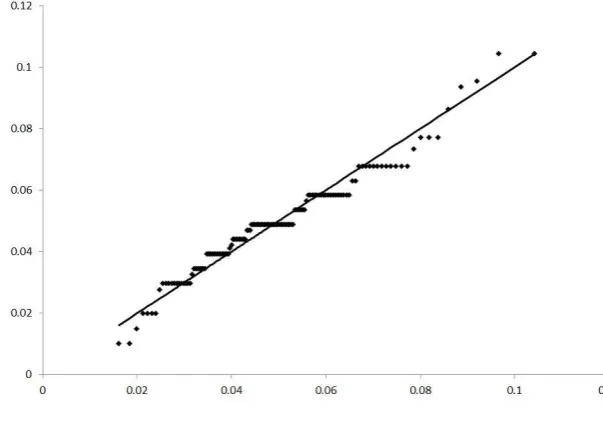
When we …t then= 131 survey responses toΓ(a, β), the maximum likelihood estimates of the parameters values areαb= 7.339,bβ= 148.53.5 In Figure 1, we present a Q-Q plot to demonstrate the goodness-of-…t between Γ bα,bβ and f λi|i∈[1,n] . By inspection, this …gure suggests that
the …t is good. More formally, we run a Kolmogorov-Smirnov test to quantify the maximum distance between the cumulative distribution functions of this gamma distribution and that of the sample data. The test statistic is 0.1078; which lies below the 5% critical level. We are, therefore, unable to reject at the standard level of statistical signi…cance the null hypothesis that the raw data are gamma distributed.
[Insert Figure 1 around here]
3 The pdf of the future value of equity portfolios
3.1 The method
The problem that the investor faces is that the “true” value ofλHis unknown. To make informed
judgements about this, she turns to the survey data. We denote byλ=n−1Pn
i=1λithe sample
mean of the survey responses. Using maximum likelihood methods to estimate the parameters of the gamma distribution, λ is also given by λ = α/b βb; see footnote 5. However, because of the …nite nature of the sample, αb and bβ will not be identical to the “true” parameters of the gamma distribution,α, β, that describes the population frequency distribution of opinions. The population mean of expert opinions, λp = α/β, will generally not equal the mean of sample
responses, λ.
Our methods involve using the observed individual responses,λ1, ..., λn, to construct a
prob-ability density function, gp(λp), for the unobserved value of λp. As we note below, there are
a number of techniques available for this; we use the one proposed by Kulkarni and Powar (2010). While we assume that the population frequency distribution of expert opinions can be well characterized through Γ(λi;α, β),there is no assumption thatgp(λp)will also be gamma
distributed; in fact, it will not be. Instead, the properties of this pdf will need to be determined using numerical methods.
Even if the investor fully knew the population mean estimate, then this would not necessarily reveal the true valueλH. The di¤erence between the population mean andλH is referred to as
the “bias”,ω,whereω=λp−λH. This is motivated by an extensive literature on analysts bias
in areas such as earnings forecasts; see, for example, Ho and Tsai (2004) and Ramnath et al. (2008). The investor must then distinguish between what she expects the bias to be, ω, from
her uncertainty over the extent of the bias,σω.
Given this, the probability density function, gλ(λH), that the investor can derive for the
true value of the equity premium based on the observed survey data comprises two elements of uncertainty. The …rst arises from the fact that only 131 experts were asked, whose aggregated views will not fully re‡ect entire expert opinion even if all responses are drawn from the same underlying statistical distribution. The second re‡ects the biasedness of analysts forecasts; even if we were to ask an in…nite number of experts, we would be unlikely to derive the true value
5 The maximum likelihood estimators that we use forbαandbβgiven the sample of responses are reported in,
ofλH. Given this, our methods …rst consider the distribution gp(λp)and then the additional
uncertainty caused by biasedness.
There are a number of known numerical techniques (Grice and Bain 1980; Jensen and Kris-tensen 1991; Wong 1993) for determining the pdf of the population mean of a gamma distribution, gp(λp)conditional on observing a …nite number of drawings from the distribution. The one that
we employ here involves transforming the data intoYi =λpi for some powerp(not to be confused
with thep subscript, which is used throughout to denote “population”). This adapts the un-derlying distribution from gamma to Gaussian. Wilson and Hilferty (1931) and Hernandez and Johnson (1980) show that, if theλis are gamma distributed, then forp= 1/3, the transformed
variables Yi will be approximately normally distributed. Hawkins and Wixley (1986) propose
insteadp= 1/4. In this paper, we follow the Optimal Power Normal Approximation Method (OPNAM) method of Kulkarni and Powar (2010) who propose usingp= 0.246 when α > 1.5 as is the case for Welch’s data. When we make the transformation Yi = λ0i.246 we …nd that
the sample meanY = 0.4712, the sample standard deviationσY = 4.40%, the skewness is -0.52
and the excess kurtosis is 1.67. A Kolmogorov-Smirnov test is unable to reject at a 5% level of signi…cance the null hypothesis that these transformed data are normally distributed.
Now denote by Yp the population mean of the transformed forecasts; Yp = E[λpi]. By the
properties of a gamma distribution (see the appendix for a proof),
Yp=E[λpi] =E[λi]p
Γ(α+p) αpΓ(α) =λ
p p
Γ(α+p)
αpΓ(α) (2)
To proceed from here, let gY (Yp) denote the pdf for the value of Yp that the investor can
construct conditional on the sample of transformed responses. Letui=Yi−Ypbe the di¤erence
between expert i’s transformed response and the transformed population mean. Because of the Gaussian nature of the Yis, we assume that the vector uwith elements ui is multivariately
normally distributed with zero mean:u∼N(0,Σu)where0is ann−vector of 0s andΣuis the
variance-covariance matrix of the elementsui.
We then use the “Unknown Σ” method of Winkler (1981) to construct con…dence intervals forYp. While we assume that the correlation between expert forecasts is known precisely (we
discuss this further below), the variance of their individual forecast errors,V ar[ui], cannot be
estimated perfectly. This is because the survey sample size of Welch is relatively small, leaving imprecision in our volatility estimate. Winkler’s method relies on observing that whenΣu is
unknown, the pdf ofYp,gY(Yp), is Student’st−distributed with δ+n−1 degrees of freedom
with meanm∗ and variances∗2
where:
m∗= 1 ′Σb−1
u Y
1′Σb−u11, s
∗2
= δ+ (m
∗1−Y)′Σb−1
u (m∗1−Y)
(δ+n−3)1′Σb−u11 (3)
δis a parameter of the Inverse Wishart distribution that is used to describe our Bayesian prior belief aboutΣu,Σbuis the sample estimate of this variance-covariance matrix,Yis ann−vector
with elements Yi and 1 is an n−vector of 1s. In the appendix we discuss in detail how we
parameterize this model based on Welch’s sample data.
Conditional on Yp being Student’st−distributed, it is now straightforward to constructLx,
the lowerx/2 quantile value forgY (Yp). Then, by reversing equation 2, the equivalent quantile
value forgp(λp),L∗x, is given by:
L∗x= (Lxα^pΓ(^α)/Γ(^α+p))1/p (4)
the combined use of the OPNAM method with Winkler’s technique for combining correlated forecasts. We …nd that there is good precision in the estimates L∗
x even with high levels of
correlation between expert forecasts.
3.2 Unbiased and independent expert forecasts
We begin by presenting results for the case when there arenindependent and unbiased (ω = 0 sogp(λp) =gλ(λH))forecasts of theH−period ex-ante equity premium,λH,each with identical
forecast error variance; V ar[ui] = σ2u for all i. This means that Σbu−|1ii = bσ
−2
u and Σbu−|1ij = 0
for j 6= i, where Σbu−|1ij denotes the element in the ith row and jth column of Σb−1
u . Under
these assumptions, which are relaxed in the next two subsections,bσ2uis estimated by the sample
variance of the transformed estimates,bσ2Y.6 Applying equation 3 is, in this case, straightforward
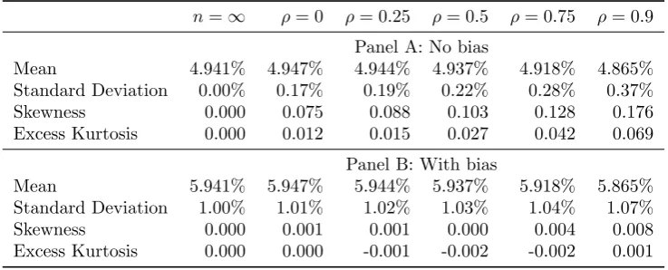
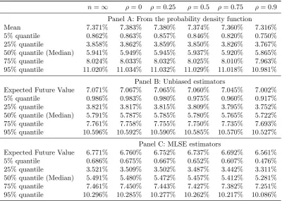
and, in Panel A of Table 1, we report the …rst four moments of gλ(λH) from the combined
application of the Winkler and OPNAM approaches.
[Insert Table 1 around here]
The …rst column,n =∞, gives the case when there is no uncertainty over the equity pre-mium and thereforeλH =bα/bβ with certainty. The second column, ρ= 0, presents the case of
uncorrelated experts. The moments can be generated here directly from the empirical estimate ofgλ(λH). The presence of uncertainty has slightly increased the mean from 4.941% to 4.947%
and is further seen through the non-zero standard deviation. The skewness and excess kurtosis remain close to zero as the number of degrees of freedom of the Student’st−distribution,δ+n−1, is over 140 in all cases. This distribution is, therefore, very similar to a normal distribution. We will return to Panel B and the …nal four columns of Panel A below.
Now consider the future value of an equity portfolio inH= 30years. In order to focus atten-tion on the equity premium it is assumed that bothrf H andΣe,theH×H variance-covariance
matrix of stock market noise, et, over the interval [0, H], are known by the investor. The
as-sumption thatΣe is known perfectly is common in this stream of literature (Blume 1974; Indro
and Lee 1997; Cooper 1998; Jacquier et al. 2003, 2005). It is considered reasonable as returns volatility can, in principle, be estimated to within any required con…dence interval provided that historic data can be obtained with su¢ciently high frequency and returns are i.i.n.d. Results are based onrf H = 0and 1′Σe1=Hσ2e with σe = 16%, which is broadly consistent with the
observed annual volatility of major stock market indices. Results are generated by randomly drawing across 10 million simulations independent values of λH, eH from their respective
prob-ability density functions and then calculating F V30 = exp (30 (λH+eH))for each simulation.
We then calculate the mean value of F V30 across the simulations and also the 5th, 25th, 50th
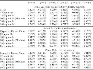
(median), 75th and 95th quantile values. In Panel A of Table 2 we present equivalent annual rates of return,R30= 30−1ln (F V30), for each of these statistics.
[Insert Table 2 around here]
The …rst column, n = ∞, presents the case when there is no uncertainty over the equity premium. In this case F V30 is lognormally distributed and so the mean value and quantiles
6 It is, in general, necessary to distinguish between the observed cross-sectional variance of the transformed sample data,σ2
Y, and the variance ofui,σ2u, which re‡ects the accuarcy of an individual forecast. For example,
if all experts make identical, but equally incorrect, forecasts thenσ2
Y = 0(all forecasts are the same) butσ2u>0
can be calculated directly from the associated normal distribution. The uncertainty over future values is clear with the 90% con…dence interval being[0.136%,9.746%]. Even the 50% con…dence interval is wide at[2.971%, 6.911%]. This, of course, understates true uncertainty as the volatility and risk-free rate processes are assumed here to be known with certainty.
The second column, ρ = 0, presents the equivalent statistics based on independent and unbiased experts using Welch’s data. Our central …nding is that the results are highly similar to the n=∞ case, although again there is a slight increase in the mean value from 6.221%to 6.231%. Given the practical di¢culties associated with accurately estimating the ex-post stock market noise process, 1′Σe1, these di¤erences seem to be of little economic importance. The
statistical rationale underlying these results is clear. The standard deviation of survey data on the equity premium is low; 1.77% in the case of Welch’s 2009 questionnaire. The central limit theorem implies that, when n = 131, the standard error associated with the mean of the distribution is only 15 basis points. If we were to use historic i.i.n.d. market returns with standard deviation of 16% per year then we would need over 10,000 years of data to achieve similar precision. Uncertainty over the true value of the equity premium, λH, is swamped by
the ex-post stock market noise,eH.
3.3 Non-independent expert forecasts
Most …nancial economists read the same academic papers, textbooks and newspapers and live within the same professional environment. There are also a number of psychological and incentive-driven reasons why an individual expert may prefer not to be too far out of line with the overall consensus. It is, therefore, highly likely that any individual forecast will be in‡uenced by the opinions of other experts. As Graham (1996, pp.193–194) notes: “economists have a tendency to ‘clump’ (make similar forecasts) ...(this)simply reveals the high positive correlation in econo-mists’ predictions that occurs because they all study the same economic fundamentals and, given similar training, are likely to interpret the inputs in a similar manner. Therefore, clumped fore-casts are quite natural; as a result, it may be important to account for correlation when combining more than one forecast”. Clemen and Winkler (1985, p.428) also note, in the context of selective judgements from di¤erent experts: “The di¤erent sources might utilize some common data, share common assumptions, or have access to some of each other’s opinions. We can represent such redundance stochastically in terms of positive dependence among the information sources.”
This e¤ect of herding, for both informational and non-informational reasons, has been well documented in both the …nancial and macroeconomic literature; see, for example, Jegadeesh and Kim (2010). Herding has also been observed in recent institutional market trading behaviour (e.g. Singh 2013). If herding also in‡uences equity premium forecasts then the information content contained with n estimates is less than would be revealed by n truly independent forecasts. Fernandez and del Campo (2010a) show that this is likely to be the case as approximately 20% (50%) of their respondents justify their answer by “historic data” (“reference to books or articles”).
To model this, following Kotz and Adams (1964), we assume that the transformed estimates, Yi, are exponentially correlated. If we rank these in ascending order, it is likely that those that
are closest together are most in‡uenced by the same schools of thought. Therefore, if we use i, jto denote the rank ordering of two estimates, we model the correlationCorr(Yi, Yj) =ρ|i−j|
error, V ar[ui] = σ2u, is the same for all experts. In this case Freeman and Groom (In Press)
prove that:7
b
Σ−1 u =κσb
−2 Y
a b 0 ... 0 b c b ... 0 0 b c ... 0
..
. ... ... . .. ... 0 0 0 ... a
(5)
a= 1
1−ρ2, b=
−ρ
1−ρ2, c=
1 +ρ2
1−ρ2, κ=
n2(1−ρ)2
−n 1−ρ2 + 2ρ(1−ρn)
n(n−1) (1−ρ)2
and this can be used in equation 3 as before. The mean is now a¤ected byρwith:
m∗=Y + (n−2)ρ
n−(n−2)ρ Y −YR (6)
whereYR= (n−2)−1Pni=2−1Yi, which is the mean of the transformed forecasts after ignoring the
highest and lowest responses. This means that forρ6= 0, m∗TY ifY
RSY, with the inequality
getting stronger for larger values of ρ. In the case of Welch’s dataYR= 0.4715>0.4712 =Y,
resulting in a mean estimate ofλH that decreases with increasedρ. This can be seen in the …nal
four columns of Panel A of Table 1. Results are presented for the …rst four moments ofgλ(λH)
at a horizon H = 30years based onρ∈ {0.25,0.5,0.75,0.9}. These can be broadly interpreted as equivalent to cases where a survey had been run with N ∈ {79,44,19,7} independent and unbiased experts respectively.8 As might be expected, the greater the correlation between ex-perts, the less sure the investor is about the true value ofλH. Therefore as ρincreases, so the
standard deviation, skewness and excess kurtosis of gp(λp) all rise. However, these e¤ects are
relatively minor in terms of economic signi…cance.
The …nal four columns of Panel A of Table 2 present the mean and …ve quantile values of R30 when expert opinion is correlated. Again, the results do not di¤er greatly from then=∞
case. Even whenρ= 0.9,the mean estimate has only fallen from6.22%to6.17%while the 90% con…dence interval widens from9.61% to9.69%compared ton=∞.
3.4 Biased expert forecasts
An additional complication arises from the fact that the population of experts may have a biased forecast of the true ex-ante equity premium; λp=λH+ω forω6= 0.
Panel B of Table 1 reports the …rst four moment of gλ(λH) when the distribution of the
population mean is independent of the bias and ω ∼ N ω, σ2ω . For illustration purposes
we set ω = −1%, σω = 1% which assumes that analysts have an expected negative bias
in estimating the equity premium, possibly as a result of placing too much weight on recent evidence of a declining cost of equity capital. A standard deviation ofσω= 1%implies that the
7 The termbσ2
u=σb2Y/κis the estimated variance of each transformed forecast error. However, it isσ2Y that
is observed and notσ2
u, and this is re‡ected in this formula. Whenρ= 0,σb2Y =bσ2u, but this is not true more
generally. See also footnote 6 and the appendix.
8 See Freeman and Groom (In Press) for a discussion on howNis calculated. This is based on the assumption that Σu is known rather than estimated with error and we do not alter that analysis here. We make this
95% con…dence interval for the true value of the bias is approximately4% in spread which we subjectively interpret as being reasonably high uncertainty. The …rst column,n=∞, presents the case when there is no uncertainty over the population mean survey response. In contrast to Panel A the standard deviation ofgλ(λH)is no longer zero but is instead equal to σω. The
in‡uence of the bias remains irrespective of how many experts we ask. However, since ω is normally distributed, there is no skewness or excess kurtosis in gλ(λH). The second column
gives the results forρ = 0. The …rst four moments can be derived directly from Panel A and the …rst two moments ofω.9 All four moments remain very similar to then=∞case, although again there is a small increase in the mean estimate from 5.941% to 5.947%. This implies that the e¤ects of the bias dominate the uncertainty over the population mean of opinions on the value of the ex-ante equity premium. When experts are non-independent as well as biased, as given in the …nal four columns of this panel, results remain similar to then=∞case. The increases in standard deviation, skewness and kurtosis caused by correlated forecasts are substantially lower than in the corresponding cases given in Panel A.
Panel A of Table 3 can be interpreted in the same way as Panel A of Table 2 but now there is a bias in the sample responses. Forn= 131 we again run 10 million simulations and take independent values of λp, eH and ω from their respective distributions to estimate the
probability density function of F VH. In the n = ∞ case the mean response is substantially
above the equivalent value given in Table 2:7.371%against6.221%. There are two reasons for this. First, the mean is shifted upwards by 1% to compensate for the expected bias. Second, the uncertainty in the true level of the bias introduces an Itô e¤ect in the mean, again pushing it up by approximately0.5Hσ2
[image:11.595.112.523.549.674.2]ω= 0.15%. For the other columns the results are similar to Panel A of
Table 2 when compared against then=∞baseline. There is a small increase in the mean for ρ= 0compared ton=∞(7.383%against7.371%), but the mean then decreases with increasing ρ. There is also some widening of the 90% con…dence interval as ρincreases, but these e¤ects do not seem to be of great practical signi…cance. Therefore, in the case of biased forecasts, understanding the properties of the bias is more important than the nature of the correlation structure.
4 The unbiased and MLSE estimators of future value
4.1 The method
To calculate unbiased and MLSE estimates ofF VH, we adapt the technique of Jacquier et al.
(2003, 2005). We take an average of thenestimates given in the sample,λ=n−1Pn
i=1λi,and
choose adjustment factorsA1 andA2 as follows:
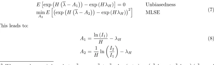
E exp H λ−A1 −exp (HλH) = 0 Unbiasedness
min
A2 E
h
exp H λ−A2 −exp (HλH) 2i
MLSE (7)
This leads to:
A1=
ln (I1)
H −λH (8)
A2=
1 H ln
I2
I1 −
λH
9 When x and y are independent, σ2
(x+y) = σ2x+σ2y, skew(x+y) = σ3xskewx+σy3skewy /σ3x+y and
kurt(x+y) = σ4
whereI1=E exp(Hλ) andI2=E exp 2Hλ .10
Following Kan and Zhou (2009), the adjustor A1 can also be used to construct the
un-biased estimator of the qth quantile of future wealth, F V
q. If λH were known then F Vq =
exp λHH+zq√1′Σe1 , where zq is the qthquantile of a standard normal distribution. If we
replaceλH with the sample mean minus the adjustor,λ−A1, then
Ehexp (λ−A1)H+zq
p
1′Σe1 −F Vq
i
= 0 (9)
which is again unbiased. It is straightforward to extend this argument to show that A2 is also
the MLSE adjustor for the qthquantile.
Notice that the problem is now di¤erent to that presented in the previous section. Here the analysis centers on understanding the properties of the sample mean of a survey drawn from a known probability density function, while in the previous section we analyzed the probability density function of the population mean contingent on survey responses. For a normal distri-bution the pdf of the population mean around the sample mean is the same as the pdf of the sample mean around the population mean. This symmetry, though, does not hold more gener-ally. For this reason, we will need to use an entirely di¤erent set of techniques in this section to the previous one.
Our contribution in this section is to extend this framework to gamma distributed survey responses. The adjustorsA1andA2in equation 8 are of the formE[exp Hλ ]andE[exp 2Hλ ].
These expressions are Hth and 2Hth moment generating functions of the probability density
function of λ. One of the main analytical conveniences of the gamma distribution is that its mgfs are well known so that if conditions arise where the sample mean is also gamma distributed, λ∼Γ(A, B), then:
E[exp xλ ] = 1−Bx −A, f(λ) =Γ(A, B), −∞< x < B (10)
This equation can be used in conjunction with equation 8 to calculateA1andA2 subject to the
respective regularity conditionsB > H andB >2H whenλ∼Γ(A, B):
A1=−
A
H ln 1− H
B −λH (11)
A2=−
A
H ln 1− H
B−H −λH
4.2 Unbiased and independent expert forecasts
In the case of independent expert forecasts λ = n−1Xn
i=1λi is a constant multiplied by the
sum of independently and identically gamma distributed random variables. This means thatλ is also gamma distributed,λ∼Γ(nα, nβ). SubstitutingA=nαandB =nβ into equation 11 gives the MLSE and unbiased adjustors. While the true parameter values, α, β are unknown, for practical purposes we recommend replacing them with their maximum likelihood estimates, b
α,βb and settingλH =bα/bβ.
Panels B and C of Table 2 give the equivalent annual rates of return,R30= 30−1ln (F V30), for
the unbiased and estimated future value and 5%, 25%, 50%, 75% and 95% quantile values. The
1 0 Notice that, if the survey data were unbiased, uncorrelated and normally distributed,λ
i∼N(λH, σ2λ),then
λ∼N λH, σ2λ/n . In this case,I1 = exp HλH+ 0.5H2σ2λ/n andI2 = exp 2HλH+ 2H2σ2λ/n . Given this
n=∞case re‡ects the situation where there is no uncertainty about the true value of the equity premium and therefore all statistics are identical across Panels A, B and C. For the independent errors case,ρ= 0, all statistics are very similar to the equivalent statistics forn=∞and their equivalents in Panel A. This again is a consequence of the low standard deviation of the survey responses and the large number of experts asked, e¤ectively removing ‘all’ uncertainty about the equity premium value. This contrasts with results presented in Blume (1974), Indro and Lee (1997), Jacquier et al. (2003, 2005) and Kan and Zhou (2009), where the e¤ects of uncertainty over the true expected return derived from historic stock returns are of considerable economic relevance.
4.3 Non-independent expert forecasts
Consider again the case of exponential correlation but now for the untransformed estimates; Corr(λi, λj) =ρ|i−j|for ordered survey responses iand j. Kotz and Adams (1964) show that
the sum ofnobservations drawn from this distribution is also approximately gamma distributed with parametersΓ(an, βn)
αn = n+
2ρ 1−ρ n−
1−ρn
1−ρ −1
n2α (12)
βn =
αn
nαβ
and thereforeλ∼Γ(αn, nβn). Notice from the previous subsection (and equation 12 for the case
ρ= 0) that if we had instead askedN independent and unbiased experts then λ∼Γ(N α, N β). By equating these two expressions, this means that the equivalent number of independent ob-servers is given byN =αn/α=nβn/β:
N = n+ 2ρ 1−ρ n−
1−ρn
1−ρ −1
n2 (13)
Settingρ∈ {0.25,0.5,0.75,0.9} givesN ∈ {79,44,19,7}. These are, to the nearest integer, the same values as given in section 3.3.
Setting A=Nαb and B =Nbβ and substituting these values into equation 11 gives the new adjustment parameters. The …nal four columns of Panels B and C of Table 2 show how this correlation structure a¤ects the equivalent annual rate of return for the unbiased and MLSE estimators of the future value and quantile values. With high values ofρ there are some clear di¤erences against then=∞case with the median future value falling from 4.941% to 4.873% (unbiased) and 4.731% (MLSE). The 90% con…dence interval is constant at 9.610% across all examples, which contrasts with the situation in Panel A where the con…dence interval widens as ρgrows larger.
4.4 Biased expert forecasts
When expert forecasts are biased and potentially correlated, by the law of iterated expectationsI1
andI2are given byI1=E E exp(Hλ)|ω andI2=E E exp 2Hλ |ω . Ifλ∼Γ(N α, N β)
we note that α=λ2p/σ2λ and β =λp/σ2λ, whereσ2λ is the variance of the population estimates.
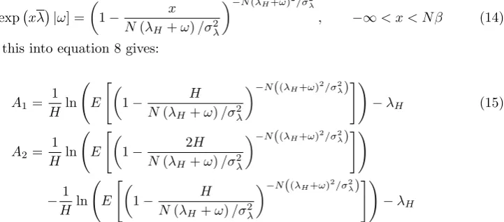
We will assume in this section that this is exactly equal to the sample variance. Then, as λp=λH+ω, from equation 10:
E[exp xλ |ω] = 1−N(λ x
H+ω)/σ2λ
−N(λH+ω)2/σ2λ
, −∞< x < N β (14)
Substituting this into equation 8 gives:
A1=
1 H ln E
"
1−N(λ H
H+ω)/σ2λ
−N((λH+ω)2/σ2λ)#!
−λH (15)
A2= 1
H ln E
"
1−N(λ 2H
H+ω)/σ2λ
−N((λH+ω)2/σ2λ)#!
−H1 ln E
"
1−N(λ H
H+ω)/σ2λ
−N((λH+ω)2/σ2λ)#! −λH
[image:14.595.127.488.199.358.2]Panels B and C of Table 3 should be interpreted in the same way as the equivalent panels in Table 2 but now there is a bias in the population estimate. Because λH is unobservable, we
replace it withλH = ^α/β^− ωfor estimation purposes. For the casen=∞, the bias adjustors
A1 = ω+ 0.5Hσ2ω and A2 = ω+ 1.5Hσ2ω. This means that, in contrast to Table 2, the
statistics in the …rst column vary between panels. These di¤erences are now of some economic signi…cance. For example, the median estimate is 5.941% under the probability density function approach (Panel A), but 5.491% when taking an MLSE estimator (Panel C). Similar results are seen when ρ= 0. As ρ increases so the di¤erences between approach start to become of real economic signi…cance. For example, with ρ= 0.9, the pdf approach gives an expected future value rate of 7.316% while the MLSE estimator is almost a full percentage point lower at 6.561%. These convert into projected future values of F V30 = $8.98 and $7.16 respectively based on an
initial investment ofF V0=$1. Therefore, when there is both herding and bias in the forecasts,
it is important to be careful when handling the survey data.
4.5 An application to optimal asset allocation
We now follow Jacquier et al. (2005) by considering how uncertainty over the true value of the equity premium might impact upon the optimal asset allocation for an investor with a power utility function and an investment horizon ofH. This investor must choose an optimal weight, W, to place in the equity market portfolio with the remainder being placed in the risk-free asset. Following Merton (1969) we assume that the future value of this mixed equity/Treasury portfolio evolves in continuous time using a simple geometric Brownian motion process:
dF V /F V = rf+W λH+ 0.5σ2e dt+W σedz (16)
Then, by Itô’s lemma:
and integrating out and using the fact thatF V0= 1:11
ln (F VH) =HRH∼N rf+W λH+ 0.5W(1−W)σ2e H, W2σ2eH (18)
By settingW = 1, it is clear that this process is consistent with the discrete time model described above. The optimization is undertaken by maximizing
max
W E[U(F VH)] = maxW E
"
F VH1−γ−1 1−γ
#
= max
W E
exp ((1−γ)HRH)−1
1−γ (19)
whereU(F VH)is the utility of …nal wealth andγis the coe¢cient of relative risk aversion. When
γ = 1, this utility function takes logarithmic form, U(F VH) = ln (F VH). This optimization
problem forγ6= 1 is equivalent to:
max
W
1
1−γexp 0.5Hσ
2
e(1−γ) (W −W2γ) E[exp(HW(1−γ)λH)] (20)
Within the assumptions of this paper:
E[exp(HW(1−γ)λH)] =E[exp(HW(1−γ) (λp−ω))]
=E[exp(HW(1−γ)λp]E[exp(−HW(1−γ)ω] (21)
= 1−HWN β(1−γ) −N α
exp −HW(1−γ) ω+ 0.5H2W2(1−γ) 2
σ2ω
resulting in the optimization problem:
max
W
1
1−γexp 0.5σ
2
eH(1−γ) (W−W2γ)−HW(1−γ) ω+ (22)
0.5H2W2(1−γ)2σ2ω 1−
HW(1−γ) N β
−N α
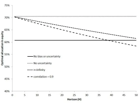
Figure 2 presents solutions to equation 22 for H ∈ [1,50] based on γ = 4, ω = −1% and
σω= 1%. The “no bias or uncertainty” line assumes thatλH = ^α/β^ and therefore there is no
allowance for the mean of the bias, the uncertainty of the bias, or the uncertainty of the population mean. This leads toW = ^α/β^+ 0.5σ2
e /γσ2ewhich is a result originally presented by Merton
(1969). This has the lowest initial weight in equity since it ignores the belief that experts are systematically over-pessimistic in their views. The “no uncertainty” line setsλH = ^α/^β− ωbut
still does not adjust for uncertainty either over the true level of the bias or the population mean. The “n=in…nity” line allows for both ω andσω but not uncertainty in the population mean.
The closed form solution for the weight in equity is now:12
W = α/^ β^− ω+ 0.5σ
2 e
γσ2
e−H(1−γ)σ2ω
(23)
Consistent with Jacquier et al. (2005) the optimal holding in equity declines with the investment horizon.13 This is caused by uncertainty over the true value of the equity premium. The
1 1 As this utility function has constant relative risk aversion, the proportion invested in the risky asset is invariant to the level of initial wealth.
1 2 The result of Jacquier et al. (2005) emerges whenN=∞,
ω= 0andσ2ω=σ2e/T.
“correlation= 0.9” line is based on numerical optimization of the full model, equation 22, with N taken from equation 13 when ρ= 0.9. The increased uncertainty over the true value of the equity premium again reduces the optimal holding in equity. At long time horizons, H = 50 years, the results are moderately sensitive to the choice of model. The “n=in…nity” line, which allows for uncertainty in the level of bias, recommends a holding in equity that is 9% lower than the “no uncertainty” case; 61.5% against 70.5%. The complete model, which also allows for uncertainty in the population mean, is a further 3% lower at 58.4%.
[Insert Figure 2 around here]
5 Designing equity premium surveys
Our empirical results allow us to make some recommendations for the future design of equity premium surveys. Our key …nding is that when experts are independent there is a striking similarity between the results obtained either when using the population mean or the sample mean even from a small survey. There seems to be little advantage to be gained from increasing the sample size beyond 10–25 respondents if expert responses are independently drawn from the same distribution. However, many surveys have very large samples; Fernandez and del Campo (2010b) have over two thousand respondents, for example.
There appear to be two potential justi…cations for requiring such a large sample size. First, we may believe that di¤erent opinions are drawn from the same distribution but with very high levels of herding. Alternatively it is possible that there are separate “schools of thought” on the equity premium. It may then be necessary to have a large sample to ensure that all important opinions are solicited in a way that is broadly proportional to their in‡uence in the overall population. If this is the case, then we …nd it somewhat surprising that current research tends to concentrate only on one particular sub-set of experts in the area; Graham and Harvey (2010) on practitioners and Welch (2001 and updates) from academics, for example. This is despite the fact that Fernandez and del Campo (2010b) show that academics, companies and practitioners tend to give di¤erent average expert responses. Taking a more holistic approach to sampling would appear more advantageous than increasing the sample size taken from a broadly homogenous subpopulation.
A potential way to design the survey so as to address issues of non-independence and schools of thought is to add a textual question that asks respondents to brie‡y explain how they arrived at their answers. We then might reasonably hypothesize that cluster analysis would reveal a rela-tionship between the numerical estimates and the textual responses. Fernandez and del Campo (2010a), who ask the question “Books or articles that I use to support this number”, provide graphical evidence that is consistent with this view. They …nd that those citing Damodaran as a key in‡uencing reference have a noticeably lower average equity premium than those using Morningstar-Ibbotson. A detailed quantitative analysis of the relationship between the empirical and written response would help enable the researcher to gain a more thorough understanding of the nature of the correlation structure that underlies the survey data. In addition the re-searcher could consider whether the textual responses represent all the main opinions on the equity premium or whether important schools of thought might be missing from, or potentially under-represented in, the sample of respondents. Finally, the textual responses may give the researcher some view on how ‘expert’ each respondent is, with the potential to remove noise-respondents on the basis of their reply.
population bias. As the ex-ante equity premium is not even observable ex-post, the issue of calibrating the bias does not obviously lend itself to direct empirical analysis. We see two possible solutions to this. The …rst is a purely literature-based approach that would draw inferences from existing studies on biases in macroeconomics and …nance. The second is to ask a connected question in an equity premium survey that could be empirically veri…ed ex-post. While both Graham and Harvey (2010) and Welch ask questions about short-term stock market movements, the volatility of realized market returns is so great that identifying the true drift parameter over such a short period of time is impossible. Given this, we would recommend a question about a variable such as GDP growth which has a much lower standard deviation. Assuming there is some correlation between over-optimism (-pessimism) with respect to short-term economic variables and long-term …nancial ones, this may enable the researcher to understand something of the properties of the equity premium bias.
6 Conclusion
Recent literature has presented the results of several surveys that ask a sample of experts for forecasts of the forward looking equity premium. The summary statistics of these responses have generated considerable interest. To our knowledge, though, no previous work has considered how optimally to combine all the data contained in any one survey. This paper bridges this gap for investors interested in investment management and optimal asset allocation problems.
We focus on two questions; what is the probability density function for the future value of an equity index tracker fund and what are the unbiased and minimum least square error (MLSE) estimates of the future value, and quantiles of the future value, of this fund? The …rst of these questions revolves around understanding the density function of the true mean of a distribution conditional on the given sample. The second, in contrast, involves understanding the density function of the mean of a random sample drawn from the population.
Following Weitzman (2001) and others we argue that equity premium survey data are well approximated by a gamma distribution. This allows us to use the numerical OPNAM technique of Kulkarni and Powar (2010) to understand the probability density function of the future value. In addition, we derive closed-form solutions for unbiased and MLSE estimates of future value, and quantiles of future value, thus extending the work of Blume (1974), Indro and Lee (1997), Jacquier et al. (2003, 2005) and Kan and Zhou (2009) when forecasts are unbiased. This is then generalized numerically for cases when expert opinions are biased.
By applying these methods to questions of future value and optimal asset allocation our central conclusion is that, unless the sample is small or expert opinions are highly correlated, then uncertainty over the population mean of forecasts is of little practical signi…cance. As a consequence, if analysts are unbiased, working with the sample mean of the survey data alone is su¢ciently accurate in most instances. If analysts are biased then the sample mean should be adjusted by the expected level of the bias but in most, if not all, cases further adjustments for uncertainty over the level of bias are small. Given the forward-looking nature of equity premium surveys and the low levels of uncertainty that they contain, we conclude that the bene…ts from using surveys to address future value problems signi…cantly outweigh their costs when compared to techniques based on historical average returns.
References
Barberis N (2000) Investing for the long run when returns are predictable. J Financ 60:225–264.
Blume M (1974) Unbiased estimators of long-run expected rates of returns. J Am Stat Assoc 69:634–663.
Clemen RL and Winkler RL (1985) Limits for the precision and value of information from dependent sources. Oper Res 33:427–442.
Cooper I (1996) Arithmetic versus geometric mean estimators: Setting discount rates for capital budgeting. Eur Financ Manag 2:157–167.
Fama EF, French KR (2002) The equity premium. J Financ 57:637–659.
Fernandez P, del Campo J (2010a) Market risk premium used in 2010 by professors: A survey with 1,500 answers. Working paper; http://ssrn.com/abstract=1606563.
Fernandez P, del Campo J (2010b) Market risk premium used in 2010 by analysts and companies: a survey with 2,400 answers. Working paper; http://ssrn.com/abstract=1609563.
Ferstl R, Weissensteiner A (2011) Asset-liability management under time-varying investment opportunities. J Bank Financ 35:182–192.
Financial Services Authority (2012) Rates of return for FSA prescribed projections. London.
Freeman MC (2011) The time-varying equity premium and the S&P500 in the twentieth century. J Financ Res 34:179–215.
Freeman MC, Groom B (In Press) Positively gamma discounting: Combining the opinions of experts on the social discount rate. Econ J.
Hawkins DM, Wixley RAJ (1986) A note on the transformation of Chi-squared variables to normality. Am Stat 40:296–298.
Hernandez F, Johnson RA (1980) The large-sample behavior of transformations to normality. J Am Stat Assoc 75:855–861.
Gollier C (2004) Maximizing the expected net future value as an alternative strategy to gamma discounting. Financ Res Lett 1:85–89.
Graham JR (1996) Is a group of economists better than one? Than none? J Bus 69:193-232.
Graham JR, Harvey CR (2010) The equity risk premium in 2010. Working paper; http://ssrn.com/abstract=1654026.
Grice JV, Bain LJ (1980) Inferences concerning the mean of the gamma distribution. J Am Stat Assoc 75:929–933.
Hung M-W, Wang J-Y (2005) Asset prices under prospect theory and habit formation. Rev Pac Basin Financ Mark Pol 8,1–29.
Indro, DC, Lee, WY (1997) Biases in arithmetic and geometric averages as estimates of long-run expected returns and risk premia. Financ Manage 26(Winter):81–90.
Jacquier E, Kane A, Marcus AJ (2003) Geometric or arithmetic mean: A reconsideration. Financ Anal J 59(Nov/Dec):46–53.
Jacquier E, Kane A, Marcus, AJ (2005) Optimal estimation of the risk premium for the long run and asset allocation: a case of compounded estimation risk. J Financ Economet 3:37–55.
Jagannathan R, McGrattan ER, Scherbina A (2000) The declining U.S. equity premium. Federal Reserve Bank of Minneapolis Quarterly Review 24(4):3–19.
Jegadeesh N, Kim W (2010) Do analysts herd? An analysis of recommendations and market reactions. Rev Financ Stud 23:901–937.
Jensen JL, Kristensen LB (1991) Saddlepoint approximations to exact tests and improved like-lihood ratio tests for the gamma distribution. Commun Stat-Theor M 20:1515–1532.
Jouini E, Marin J-M, Napp C (2010) Discounting and divergence of opinion. J Econ Theory 145:830–859.
Kan R, Zhou G (2009) What will the likely range of my wealth be? Financ Anal J 65(July/August):68-77.
Kotz S, Adams JW 1964. Distribution of sum of identically distributed exponentially correlated gamma-variables. Ann Math Stat 35:277–283.
Kulkarni HV, Powar, SK, 2010. A new method for interval estimation of the mean of the gamma distribution. Lifetime Data Anal 16:431–447.
Lettau M, Ludvigson SC, Wachter JA (2008) The declining equity premium: What role does macroeconomic risk play? Rev Financ Stud 21, 1653–1687.
Mehra R, Prescott EC (1985) The equity premium: a puzzle. J Monetary Econ 15:145–61.
Mehra R, Prescott EC (2003) The equity premium in retrospect, in Constantinides GM, Harris M, Stulz R (eds) Handbook of the Economics of Finance, Volume 1B: Financial Markets and Asset Pricing (North Holland).
Merton R (1969) Lifetime portfolio selection under uncertainty: The continuous-time case. Rev Econ Stat 51:247–257.
Ramnath S, Rock S, Shane P (2008) The …nancial analyst forecasting literature: A taxonomy with suggestions for further research. Int J Forecasting 24:34–75.
Rapach DE, Zhou G (2011) Forecasting stock returns. Working paper, Saint Louis University.
Singh V (2013) Did institutions herd during the internet bubble? Rev Quant Financ Acc 41: 513-534.
Tsai H-J, Wu Y (In Press) Optimal portfolio choice with asset return predictability and non-tradable labor income. Rev Quant Financ Acc.
Weitzman ML (2001) Gamma discounting. Am Econ Rev 91: 260–271.
Weitzman ML (2010) Risk-adjusted gamma discounting. J Environ Econ Manag 60:1–13.
Welch I (2000) Views of …nancial economists on the equity premium and other issues. J Bus 73–4:501–537.
Wilson EB, Hilferty MM (1931) The distribution of Chi-squares. P Natl Acad Sci USA 17:684– 688.
Winkler RL (1981) Combining probability distributions from dependent information sources. Manage Sci 27:479-488.
7 Appendix
In this appendix, we present further details of the Kulkarni and Powar (2010) OPNAM method for estimating the density function of the mean of a gamma distribution conditional on a …nite sample, the Winkler (1981) method for combining correlated expert forecasts, and the application of these two methods to the problem at hand. We also, by simulation, demonstrate the accuracy of these two techniques.
7.1 Transforming the data
The OPNAM method relies on the fact that if the underlying dataλi ∼Γ(α, β)thenYi =λpi
will be approximately normally distributed for p = 0.246 provided that α > 1.5. The …rst four moments of Yi are known in closed form — we derive the …rst two here and note that the
equivalent equations for skewness and kurtosis are given on page 437 of Kulkarni and Powar (2010). The pdf of a gamma distribution is given by:
g(λi)∼Γ(a, β) =
βα Γ(a)λ
α−1 i e−βλ
i
(24)
So, the expectation ofYp=E[λpi]is given by
Yp=
Z ∞
0
λpi
βα Γ(a)λ
α−1 i e−βλ
i dλi=
Z ∞
0
βα Γ(a)λ
p+α−1 i e−βλ
i
dλi (25)
= Γ(a+p) βpΓ(a)
Z ∞
0
βp+α Γ(a+p)λ
p+α−1
i e
−βλi dλi
The transformation in the last line is ‘trivial’ in the sense that it is just multiplying both the numerator and denominator by βpΓ(a+β)and then rearranging. The purpose of this trivial transformation is to ensure that the term within the integral is identical to the probability density function of a gamma distribution with parameters α+pandβ. Clearly as this is the integral over the whole support of well-de…ned pdf, it must equal one. Therefore:
Yp =
Γ(a+p) βpΓ(a) =
α β
p
Γ(a+p)
apΓ(a) =E[λi]
p Γ(a+p)
apΓ(a) (26)
and this is equation 2 in the body of this paper.
The cross-sectional variance of the forecasts is given byσ2 Y =E
h
λ2ipi−E2[λp
i], which follows
directly from the preceding argument:
σ2 Y =
1 βpΓ(α)
2
Γ(α+ 2p)Γ(a)−Γ2(α+p) (27)
Similar expressions follow for the skewness and excess kurtosis and Kulkarni and Powar note that these depend on α and p but not β. Therefore the choice of p depends onα only. For α > 1.5, they select p = 0.246 so as to get the skewness and excess kurtosis jointly close to zero. Their method is an approximation, though, and therefore theYisare only approximately
normally distributed even if theλisare perfectly gamma distributed.
A key feature to notice is that this transformation from gamma to normal does not depend on the generating process for the underlyingλis. Therefore this applies equally well to correlated as
131 normally distributedN(0,1)and exponentially correlated random variables. We then con-vert these to correlated uniform random variables using the cumulative density function of the standard normal distribution. Finally, we take an Inverse Gamma function to convert again into correlated gamma distributed random variables,λi.14 We then construct the transformations
Yi =λ0i.246and calculate the …rst four moments of the transformed forecasts.
In Table A, we report our results. In Panel A we present information on the initial correlation structure that is put into the Cholesky decomposition and the estimated correlations between λi and λi+1 and Yi and Yi+1 across the simulations (where i = 50 is chosen at random for
illustrative purposes). This clearly demonstrates that the correlation structure remains almost entirely una¤ected by the transformations that we undertake — we discuss this point further below. In Panel B we present the median values of the …rst four moments of theYis across these
simulations, along with lower 2.5% and upper 97.5% simulated values. These are compared against the theoretical values given above and in Kulkarni and Powar (2010).
[Include Table A around here]
For all values ofρconsidered, the theoretical predictions lie within the 95% con…dence interval and close to the observed median values. This shows the robustness of the power transformation to correlation in the experts’ forecasts.
7.2 Constructing con…dence intervals forα/β
The purpose of using the OPNAM method is to construct con…dence intervals, L∗
x, for the
population mean (rather than survey mean),λp, of expert responses. To do this, we …rst construct
con…dence intervals,Lxfor the population mean,Yp(as given in equation 26) of the transformed
responses and then use equation 4 to constructL∗
x. We do this using the “UnknownΣ” method
described in Winkler (1981). While we assume that the correlation between experts,ρ|i−j|, is known perfectly, the sample cross-sectional variance of transformed forecasts,bσ2Y,will di¤er from
the population cross-sectional variance of transformed forecasts,σ2
Y. AsΣu|ij =σ2Yρ|i−j|, this
introduces sampling error into our estimateΣbu.
To overcome this problem, following Winkler (1981), we form a Bayesian prior that the “true” variance-covariance matrix is Inverse Wishart distributed with parameter valueδ:
f Σ|Σb, δ ∝ Σ−1
δ+2n
2
exp −δ2tr Σ−1Σb (28)
where | | is a matrix determinant andtr( )is a matrix trace. In this case, as discussed in the body of the paper,Yp is Student’s t−distributed conditional on the transformed sample data,
withδ+n−1degrees of freedom and meanm∗and variances∗2
,as given in equation 3. In the case of exponential correlation, Σb−1
u is given in equation 5 and, from here, the expressions for
1 4 As discussed in early footnotes, it is necessary to distinguish between the cross-sectional variation of responses,
σ2
Y,and the variance of individual forecast errors,σ2u;σ2u=σ2Y/κwhereκ= 1whenρ= 0. To account for this
distinction, the Inverse Gamma function is calibrated to α∗and
β∗, where
α∗
=ακ−1 and β∗
=βκ−1. The
m∗ ands∗2
can be simpli…ed by noting that:
1′Σb−1 u 1=κbσ
−2 Y
n(1−ρ) + 2ρ
1 +ρ , Y
′Σb−1 u 1=κσb
−2 Y
nY −ρ(n−2)YR 1 +ρ
Y′ΣYb =κbσ−2 u
nV +ρ2(n−2)VR−2ρ(n−1)Z
1−ρ2 (29)
V = 1 n
n
X
i=1
Yi2, VR=
1 n−2
nX−1
i=2
Yi2, Z=
1 n−1
n−1
X
i=1
YiYi+1
Therefore the only complexity that arises when operationalizing equation 3 is identifying the parameter δ.
7.3 Estimatingδ
To estimateδ, we draw upon the commonly observed parallel between the Inverse Wishart dis-tribution and the Inverse Gamma disdis-tribution. We start with the standard assumption that the relationship between the cross-sectional sample variance and cross-sectional population variance is given by a Chi-squared distribution withv−1degrees of freedom;(v−1) bσY2/σ2Y ∼χ2v−1.
We explain below howv is estimated. This means that:
b
σ2Y
σ2 Y
∼ χ
2 v−1
v−1 =Γ
v−1 2 ,
v−1
2 (30)
which is a gamma distribution with both shape and rate parameters equal to(v−1)/2. It then follows that σ2
Y ∼ Γ−1 v−21, v−1
2 σb 2
Y , where Γ−1(, ) is an inverse gamma function and the
second parameter is now the scale parameter. Then, by the properties of the Inverse Gamma distribution:
V ar σ2Y =
2(v−1)bσ2Y
(v−3)2(v−5) (31)
To link this to the Inverse Wishart distribution that forms the basis for the “Unknown Σ” method of Winker, we note σ2
Y =Σu|ii, and therefore the variance of this variable is given by
V ar Σu|ii . For an Inverse Wishart distribution, the relationship between the precision of our
estimate ofΣu|ii and bσ2Y is given by:
V ar Σu|ii =
2δbσ2Y
(δ−2)2(δ−4) (32)
and by comparison of equations 31 and 32 it is clear thatδ=v−1.
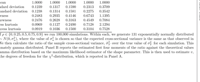
To estimate v we take a numerical approach. We run 100,000 simulations for all ρ ∈ {0,0.25,0.5,0.75,0.9}. In each case, we draw 131 exponentially correlated Normal random error termsui∼N 0, σ2Y , where for simulation purposes,σ2Y =bσ
2
Y. For each simulation,s, we then
calculate the cross-sectional variance of the error term,σb2sY. We then take the maximum likeli-hood estimator of(v−1)/2, the shape parameter of the gamma distribution, across the 100,000 simulations.15 The values that emerge forv for ρ∈ {0, 0.25, 0.5, 0.75,0.9} are, to the nearest integer,v={131,115,81,40, 17}. These results are reported in more detail in Table B. This
table also compares the …rst four moments ofbσ2Y/σ2Y against those of aΓ((v−1)/2,(v−1)/2)
distribution.
[Include Table B around here]
7.4 Accuracy of the method
To demonstrate the accuracy of our joint use of the OPNAM method and Winkler’s “Unknown Σ” technique for combining correlated forecasts, we run a further set of simulations. Within each of 100,000 simulations, for each value ofρ∈ {0,0.25,0.5,0.75,0.9}we draw 131 values ofYifrom
an exponentially correlated normal distribution N(E[Yi], V ar[Yi]). As discussed above, both
E[Yi]and V ar[Yi] are known in closed form as functions ofα, β. For simulation purposes, we
use the values ofαandβthat are empirically estimated from Welch’s data. For each simulation, we use a combination of the Winkler (1981) “Unknown Σ” method described above with the Kulkarni and Powar method to derive one-sided upper and lower 0.5%, 1%, 1.5%,..., 9.5% and 10% con…dence intervals forα/β. We then count the proportion of simulations where the initial value ofα/βlies outside the estimated con…dence interval. These results are reported in Table C.
[Include Table C around here]
As can be see, in all cases there is very close agreement between the estimated con…dence level and the proportion of simulations whereα/βlies outside the estimated con…dence interval. This demonstrates the robustness of the method that we use to correlation in the forecasts.
7.5 The correlation structure
Finally, we turn to the correlation structure and demonstrate again that there is close agreement between the assumed correlation structure for the untransformed and transformed estimates (see also Panel A of Table A above). For the case ofρ= 0.9, we simulate 131 correlated Yis using
the standard Cholesky decomposition approach and then construct values ofλi=Yi1/0.246. We
repeat these simulations 10,000 times. In Figure 1 we present the correlation betweenλ1andλj
forj∈[2,131]across the 10,000 simulations. This is compared against Corr(Y1, Yj)andρ|i−j|,
which is the theoretical value under exponential correlation.
[Include Figure A around here]
It is clear that the correlation structure of the λisis also very close to being exponentially