Multilevel Modelling with Spatial Interaction Effects with Application to an Emerging Land Market in Beijing, China

Multilevel Modelling with Spatial Interaction

Effects with Application to an Emerging Land

Market in Beijing, China

Guanpeng Dong1_{*, Richard Harris}2_{, Kelvyn Jones}2_{, Jianhui Yu}3_*

1Sheffield Methods Institute, Faculty of Social Sciences, The University of Sheffield, Interdisciplinary Centre of the Social Sciences (ICOSS), 219 Portobello, Sheffield, S1 4DP, United Kingdom,2School of

Geographical Sciences, University of Bristol, University Road, Bristol, BS8 1SS, United Kingdom,3Key Laboratory of Regional Sustainable Development Modelling, Institute of Geographical Sciences and Natural Resources Research, CAS, Beijing, China

*[email protected](GD);[email protected](JY)

Abstract

This paper develops a methodology for extending multilevel modelling to incorporate spatial interaction effects. The motivation is that classic multilevel models are not specifically spa-tial. Lower level units may be nested into higher level ones based on a geographical hierar-chy (or a membership structure—for example, census zones into regions) but the actual locations of the units and the distances between them are not directly considered: what mat-ters is the groupings but not how close together any two units are within those groupings. As a consequence, spatial interaction effects are neither modelled nor measured, con-founding group effects (understood as some sort of contextual effect that acts‘top down’ upon members of a group) with proximity effects (some sort of joint dependency that emerges between neighbours). To deal with this, we incorporate spatial simultaneous auto-regressive processes into both the outcome variable and the higher level residuals. To assess the performance of the proposed method and the classic multilevel model, a series of Monte Carlo simulations are conducted. The results show that the proposed method per-forms well in retrieving the true model parameters whereas the classic multilevel model pro-vides biased and inefficient parameter estimation in the presence of spatial interactions. An important implication of the study is to be cautious of an apparent neighbourhood effect in terms of both its magnitude and statistical significance if spatial interaction effects at a lower level are suspected. Applying the new approach to a two-level land price data set for Beijing, China, we find significant spatial interactions at both the land parcel and district levels.

Introduction

Many geographical data sets have multilevel structures—for example, houses nested into districts into regions in an urban housing market, or cities nested into regions, that are further nested into countries. Using the language of the multilevel modelling literature, the finer spatial scale at

OPEN ACCESS

Citation:Dong G, Harris R, Jones K, Yu J (2015) Multilevel Modelling with Spatial Interaction Effects with Application to an Emerging Land Market in Beijing, China. PLoS ONE 10(6): e0130761. doi:10.1371/journal.pone.0130761

Academic Editor:Yanguang Chen, Peking UIniversity, CHINA

Received:January 5, 2015

Accepted:May 22, 2015

Published:June 18, 2015

Copyright:© 2015 Dong et al. This is an open access article distributed under the terms of the

Creative Commons Attribution License, which permits unrestricted use, distribution, and reproduction in any medium, provided the original author and source are credited.

Data Availability Statement:All relevant data are within the paper and its Supporting Information files.

Funding:This work was supported by National Nature Science Foundation of China (No. 41201169; 41230632). The funders had no role in study design, data collection and analysis, decision to publish, or preparation of the manuscript.

which an outcome variable is measured is termed the lower level whereas the more aggregate spatial scale is called the higher level. The multilevel modelling anticipates both differences between the higher level units and correlations within those units. The correlations within units are expected because their members are assumed to be affected by the same aggregate effects. The within group correlation is usually termed group dependence. The existence of group depen-dence among lower level units violates the classic assumption of independepen-dence in a standard regression analysis, raising the risk of inefficient model estimation and incorrect inference [1].

In a geographical setting, group effects are often termed place, contextual or neighbourhood effects. Multilevel models (MLM) have been widely applied to model and identify the existence of these effects [2]. Contextual effects refer to the idea that local contexts (represented by the higher level units) could affect the outcomes of lower level units belonging to them even condi-tioning on both higher and lower level covariates. For example, in geographical studies of health, the local context where individuals live has been found to make a difference in terms of a wide range of people’s health outcomes—people with nearly identical personal attributes and socio-economic characteristics but who live in different areas can have divergent health conditions [3].

However, in a geographical setting, it is not only the contextual effects that create the group dependence. Spatial interactions between the lower level units that are closely co-located (inter-actions that are termed spatial spillover effects in the spatial econometrics literature) can con-tribute to the correlations amongst group members. This issue has been rarely discussed in the multilevel modelling literature. Indeed, in its most common specification, the MLM is not really an explicitly spatial form of analysis at all. This can be seen by the absence of a spatial weights matrix giving the proximity between units, whether it is contiguity based, or based on Euclidean distance defining the‘n’nearest neighbours. No geographical information as such is passed to the MLM beyond the grouping of lower level units into higher level ones.

For geographically referenced data sets, we might expect that the outcome at a particular location would be influenced by its surrounding locations with the intensity of this influence being determined by the geographic proximity. This spatial interaction effect is nonetheless dif-ficult to model using classic multilevel models. This is because, at the lower level, the correla-tion structure among observacorrela-tions is defined as discontinuous, bounded by the geographical boundaries of the higher level units. Consequently, two lower level units located either side of a boundary are assumed to be independent even though they are in close geographical proximity. Secondly, the (unobserved) contextual effects (which are the higher level residuals) are pre-sumed to be independent. Consequently, any spatial proximity effects at the higher level are not taken into account. Whereas both contextual and spatial proximity effects may affect the outcome of interest, the MLM can only consider the first effect, which may be confounded with the second and incorrectly estimated as a result.

performance of this approach under various scenarios is assessed through extensive Monte Carlo simulations.

The remainder of this paper is organised as follows. First, principles of the classic MLM and existing efforts to incorporate spatial interaction effects into the MLM briefly are reviewed. We then describe the approach developed in [8] and evaluate the validity of this approach against the MLM via a simulation study. Next, the proposed method is employed to investigate the land market in Beijing, China and the results are compared with that from a classic MLM.

Materials and Methods

Multilevel models and spatial effects

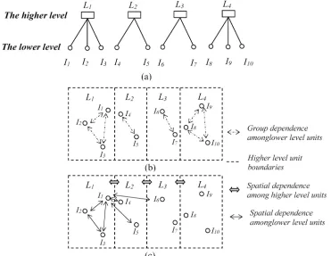
Consider a two level geographically hierarchical dataset where there areNlower level units nested intoJhigher level units that each containsnjlower level units. A simplified graphical typology of this structure is shown inFig 1a. There are four higher level units (L1toL4) and ten lower level units (I1toI10).Fig 1b) and 1c are the corresponding geographic representations of Fig 1a.

Following [1], a random intercept MLM is specified as,

yij¼β0þxTijβþxjTγþujþεij varðε_ijÞ ¼s2_e;varðujÞ ¼s2u covðε_ij;ujÞ ¼0;covðεijεi0j0Þ ¼0ifj6¼j0

ð1Þ

whereiandjindicate the lower and higher levels, respectively,yijis the outcome variable,xij

Fig 1. A two level data structure shown hierarchically and also as a map.

andxjrefer to the lower and higher level independent variables,βandγare the corresponding regression coefficient vectors to estimate (βat the lower level,γat the higher level),εijis the lower level residuals, assumed to follow an independent normal distribution, N (0,σe2), anduj are the higher level residuals also assumed to follow an independent normal distribution, N (0,

σu2). It isujthat, in a geographical setting, are taken to measure unexplained contextual effects. The covariance between lower level units in the same higher level unit is cov(yij,yi’j) = cov(uj+

εij,uj+εi’j) =σu2wherei’denotes different lower level units in thejth higher level unit. The non-zero covariance indicates the group dependence at the lower level. Moreover, the intensity of the group dependence is quantified by cov(yij,yi’j) /var(yij) =σu2/(σu2+σe2), which is known as the variance partitioning coefficient (VPC) [1,2]. As illustrated inFig 1b, there are tions among the lower level units in the same higher level unit and the strength of these correla-tions isσu2/ (σu2+σe2) for each higher level unit.

The possibility of a proximity based spatial interaction effect is illustrated inFig 1c. At the lower level, consider the example ofI1inL1. Rather than just assuming it is correlated withI2 andI3as in the MLM, it could also interact withI4,I5andI6because they are nearby. In contrast, becauseI7,I8,I9andI10are far fromI1, we might assume their spatial proximity effect onI1will reduce to zero. With respect to the magnitude of the interactions, it seems that the intensity of correlation betweenI1andI2should be larger than that betweenI1andI3because the first pair has less of a geographical separation. Moreover, at the higher level,L1,L2,L3andL4are also potentially interacting with each other. Note, again, that a classic MLM approach does not allow for proximity effects other than the grouping of lower level units into higher level ones.

Existing work on multilevel models with spatial interactions

In the geographies of health literature, some have recognised both the contextual effects and the spatial interaction effects and have modified the classic MLM accordingly. Langford et al. (1999) add an additional lower level spatial random variableviintoEq (1)[9]. It is a weighted sum of a set of independent random effectsvfrom neighbouring units such that,

vi¼

X

k6¼iwikvk ð2Þ

wherewikare entries of a row-normalised spatial weights matrixWat the lower level, defined by geographic distances. The random effectsvare distributed as N (0,σv2). Through this adjustment to the MLM, spatial interaction effects at the lower level are modelled. This can be seen from the conditional covariance matrix ofy[9],

covðyjx;β;γ;uÞ ¼s2_eINþsε;vðWþWTÞ þs2vWWT ð3Þ

whereσε,vis the covariance betweenεandv,xincludes both lower and higher level

covari-ates andINis an identity matrix with order ofN.

In a similar vein, Browne et al. (2001) propose a multiple-classification, multiple-member-ship, multilevel model (MMMC) based on their formal definition of classifications to tackle spatial dependence [10]. The idea is to consider the neighbours for each lower level unit as an additional multiple membership classification. Using their notation, a MLM with spatial inter-actions can be specified as,

yi¼β0þxTiβþu ð2Þ ContextðiÞþ

P

k2NeighbourðiÞwikvkð3Þþεi uðContextðiÞ2Þ eNð0;s2uÞ;vkð3ÞeNð0;s2vÞ;εieNð0;s2eÞ

ð4Þ

random effects andvk(3)is the neighbourhood level random effects. The departure from the modification in [9] is the assumption of independence betweenvandε. Therefore,σε,vinEq (4)is zero. This technique has been employed to investigate the impact of the network depen-dence on students' educational attainment [11]. Other modifications of the MLM directly con-ceptualise the random effectviinEq (2)as a conditional autoregressive process or a Gaussian spatial process [10,12,13].

To summarise, the above modifications to the classic MLM take a conditional approach. That is, an assumption of conditional independence of the outcome under study is imposed, indicating that changing characteristics of covariates (xij) will not influence outcomes of nearby units. Therefore, these methods are not so useful when substantial spatial interaction effects are expected, when the outcome at one location is directly related to the outcomes at surrounding locations. Possible simultaneity or endogeneity inherent in the outcome variable under study cannot be properly modelled using the above adjustment to the MLM. Moreover, spatial inter-action effects among the higher level units are generally not taken into account.

Proposed multilevel models with spatial interaction effects

With the limitations of the existing work on incorporating spatial interaction effects into the MLM in mind, our proposal is to integrate simultaneous autoregressive (SAR) processes for both the response variable and higher level residuals into the classic MLM. The SAR process has been extensively discussed in the spatial econometrics literature and widely used in geo-graphical research [14,15,16,17,18]. A key characteristic of a SAR process is that it allows the observed value at a particular location to be directly dependent on the values observed at sur-rounding locations (or lagged y), in this way allowing for an interaction (or spatial spillover) effect to be both specified and measured. Following [8], the MLM with spatial interaction effects is specified as,

y¼rWyþXβþZγþDθþε

θ¼lMθþu

D¼

l1 0 0

0 l2 0

0 0 lJ

2 6 6 6 6 6 6 6 4 3 7 7 7 7 7 7 7 5

ð5Þ

whereyis anNby 1 column vector of outcome variable values;X, anNbyKmatrix, denoting the lower level covariates;βis aKby 1 vector of regression coefficients to estimate;Zis anNby Pmatrix consisting of higher level variables;γis the correspondingPby 1 coefficient vector;W is the spatial weights matrix among lower level units as inEq (2);ρis a spatial autoregressive parameter indicating the strength of spatial interactions at the lower level;Δis anNbyJblock diagonal design matrix with column vectors of ones; andεdenotes the lower level residuals, which are distributed as N (0,σe2).

TheJby 1 vector of higher level residualsθ[θ1,θ2,. . .,θJ] represent the random contextual effects. The residualsuare distributed as N (0,σu2) and are assumed to be independent ofε. LikeW,Mis also a row-normalized spatial weight matrix but at the higher level. The parameter

FromEq (5)we see that the conditional expectation ofyis,

EðyjXβ;ZγÞ ¼ ðINrWÞ 1_ð

XβþZγÞ ð6Þ

which means that changing the values of the covariates at one location in the proposed model will affect not only its own outcomes but also outcomes at other locations because of (IN–ρW)

-1_{. Also, the substantial spatial interaction effect can be seen from the marginal effects for each}

covariate. For example, the marginal effects for a lower level variablexkare,

@y=@xk¼ ðINrWÞ 1

INβk¼SkðWÞINβk SkðWÞ ¼ ðINrWÞ

1 _{¼ ð}

INþrWþr2W2þ. . .Þ

ð7Þ

which is the same as for a standard spatial SAR regression model because the contextual effects

θare assumed to be independent ofX.

The proposed model is, therefore, hierarchical—allowing for parameter estimates at two lev-els. It also is spatial—estimating a spatial interaction effect and at two levlev-els. The model is implemented via a Bayesian Markov Chain Monte Carlo (MCMC) simulation approach. Details on full conditional distributions for each parameter are provided in [8]. The MCMC sampler for implementing the proposed method is coded using the R language in the subse-quent analyses (seeS1 Appendix).

Simulation study

In this section, a series of Monte Carlo simulations are conducted to evaluate the performance of the proposed methodology and to show how the issue of spatial interaction deteriorates the estimation from a MLM. The data generating process follows a MLM with spatial interaction effects (Eq (5)). The experiment includes 20 scenarios based on different combinations of spa-tial autoregressive parametersρ[0, 0.2, 0.4, 0.6, 0.8] andλ[0.4, 0.6, 0.8, 0.9].

Data generation

The spatial structure used is based on the real-world geography of the residential land parcels dataset in Beijing, China. There are 1117 land parcels (the lower level units) situated into 111 districts (Jiedao, the higher level units) in Beijing and we have both the geographic coordinates of those land parcels and the boundaries of the districts (Fig 2). A detailed description of the data is provided later.

The spatial weights matrix at the land parcel levelWis specified as,

Wij¼

expððdij2Þ=d2Þ if dijd

0 if dij>d

ð8Þ

(

,which is an exponentially decay function wheredis the distance threshold, set to 1.5km. This is the distance at which the correlations between land prices become negligible and was deter-mined through an exploratory analysis using variograms [19,20]. In the following empirical land price model, we also conducted a sensitivity analysis using different threshold distances such as 2km and 2.5km; the model estimation results were similar. The Euclidian distance between land parcels isdij. The district level spatial weight matrixMis based on the contiguity of the 111 districts. BothWandMare row-normalized in the subsequent analyses.

district effects are generated using:

θ¼ ðIlMÞ1u; u_eNð0;s2_uÞ ð9Þ

where the variance of the higher level residuals,σ_u2, is set to 0.4. The higher level spatial inter-action termλis sequentially set to [0.4, 0.6, 0.8, 0.9], indicating increasing intensity of spatial interactions at the higher level. The second step is to generateYby using:

Y¼ ðIrWÞ1ðXβþDθþεÞ; ε_eNð0;s2_eÞ ð10Þ

whereX= [1,X1,X2,X3], the variance of the lower level residuals,σe2is set to 0.8 and the lower level spatial interaction termρto [0, 0.2, 0.4, 0.6, 0.8]. Therefore, we have 20 scenarios in total using different combinations of values ofρandλ.

Given the above setup, 200 simulated data samples were generated for each scenario. For each data sample, estimates of the model parameters were obtained using classic MLM and with our spatial extensions. The relative performance of these two models are assessed by the bias and root-mean-square error (RMSE) of the regression coefficientsβ, two spatial autore-gressive parameters (ρandλ) and two variance parameters (σe2andσu2), presented as a per-centage of their true values [21]. For each data replication, the inference of the proposed method is based on 10000 draws with the first 5000 discarded to allow the MCMC sampler to converge. Diffuse or quite non-informative priors were employed for model parameters,β,ρ,

Fig 2. The price per area of residential land parcels leased between 2003 and 2009 within the study area of Beijing, China.

λ,σe2andσu2while the initial values were draw randomly from their corresponding distributions.

Results and Discussions

Simulation results

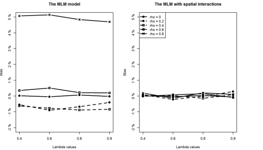
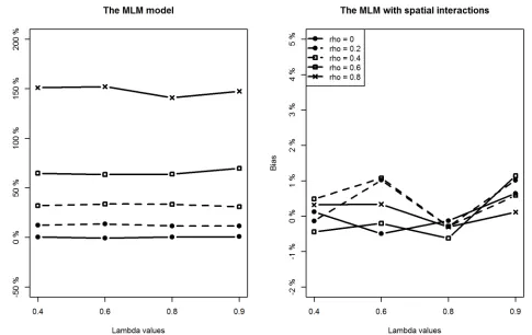
With respect to the estimation of regression coefficients, the relative bias of the proposed model is negligible in most of the scenarios. In only a few scenarios, the estimation bias of the intercept term seems slightly large, reaching about 10% (still much smaller than the bias from the classic MLM model). In contrast, the situation is more complicated for the MLM. For lower level covariates (X1andX2), the MLM provides slightly larger biased estimates when compared to the proposed method in all scenarios (Figs4and5). However, of particular note are the estimates for the intercept and the higher level covariate effect, which are highly biased when the spatial interaction effect at the lower level is large. For example, whenρis above 0.4, regardless of the intensity of spatial interaction effects at a higher level, estimation biases for the intercept term and the higher level covariate are very noticeable (Figs3and6).

Additionally, we can see that estimation biases of regression coefficients are positively related to the strength of spatial interactions at a lower level. Recall that in many application studies, higher level covariate effects are interpreted as (observable) contextual or neighbour-hood effects. An important implication of this simulation study is to be cautious of the identi-fied neighbourhood effect in terms of both its magnitude and statistical significance if spatial interaction effects at a lower level are suspected.

Fig 3. Comparing estimation results of the intercept term between classic MLM and the MLM with spatial interactions (Note the different y-scales).

As for the estimation precision indicated by the RMSE values for each covariate, we see the proposed method provides consistently more precise estimates for all the regression coeffi-cients than the MLM does in most of the scenarios. The better performance of the proposed methodology is expected. We have, after all, generated the data using the proposed model. Nev-ertheless, the simulation serves to demonstrate an important point: if there are spatial interac-tion effects at the lower and higher levels, the MLM appears to produce biased and imprecise estimates for the regression coefficients.

As for the spatial autoregressive parameters (which can be estimated only with the proposed methodology, not the MLM), the estimation biases forρandλare also quite small in all scenar-ios. The estimation bias of the higher level spatial autoregressive parameterλis slightly larger than that ofρin each scenario. This might be related to the relatively small number of higher level units [17,22]. The lack of a sufficient effective sample size at the higher level also results in a larger RMSE forλwhen compared toρ. Overall, the proposed method performs well in retrieving the two true spatial autoregressive parameters.

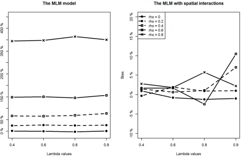
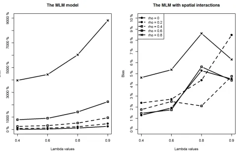
With respect to the estimation of the two variance parameters, the proposed method per-forms well by providing accurate and precise estimates for both the higher level and lower level variances. In contrast, the MLM tends to overestimate their sizes because of unmodelled spatial interaction effects. The degree of the upward bias is striking for the higher level variance parameterσu2when the intensity of spatial interactions at the lower level is relatively large (Fig 7). For example, whenρis about 0.6, the relative bias reaches about 800%. In addition, the degree of bias forσu2is positively related to the intensity of spatial interaction effects at both levels. This implies that in the presence of medium-to-strong degree of spatial interactions at a

Fig 4. Comparing estimation results of_β1between classic MLM and the MLM with spatial interactions.

lower level, estimation of higher level variance from classic MLM is not reliable at all and nor is the usual variance partitioning coefficient (VPC) measure.

To access the accuracy of retrieving the (unobserved) contextual effectsθin the proposed method and in the MLM, for each of the 200 data replications in each scenario (20 in total) we calculate the correlation coefficients between the posterior means ofθfrom the two models and their true values. For all the 4000 (200×20) data replications, the mean correlation coeffi-cient from the proposed method is 0.916 with an interquartile ranging from 0.888 to 0.949, indicating that the proposed method can retrieve the true higher level random effects accu-rately. In contrast, the mean correlation coefficient from the MLM is 0.781 with an interquar-tile ranging from 0.696 to 0.892.

Land price modelling results

Data and variables. In this section, we apply the proposed methodology to analyse an emerging land market in Beijing based on all residential land parcels from 2003 to 2009 leased by the government. The outcome variable is the leasing price per square metre of each residen-tial land parcel, adjusted by using the consumer price index (CPI). The land parcel level covari-ates used here are the land parcel size (Logarea) and the proximity of each land parcel to the nearest subway stations (LogDsubway), to elementary schools (LogDele), to green parks (LogDpark), to rivers (LogDriver) and to the central business district (LogDcbd). Year dum-mies (Year04—Year09) are also included in the model to control for fixed period effects, with the year 2003 as the baseline. The district level covariates are the population density of each dis-trict (Popden), the proportion of houses built before 1949 (Buildings1949), and the number of

Fig 5. Comparing estimation results of_β2between classic MLM and the MLM with spatial interactions.

violent crimes taking place per 1000 people (Crimerate). The natural log transformation is applied to the proximity measures to mitigate the potential problem of heteroskedasticity. The land price data used here is inS1 Datasetand a brief summary of the complete set of variables, including their definition, mean and standard deviation is presented inTable 1.

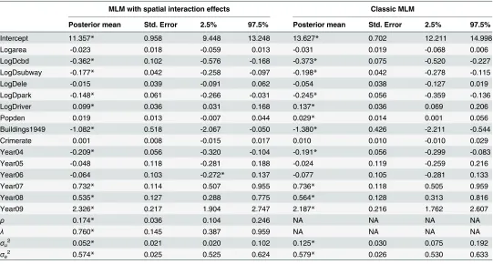
Estimation results. The estimation results from the proposed model and the MLM are provided inTable 2. We also examined the potential problem of multicollinearity using the variance inflation factor (vif) scores for the predictor variables. There is no evidence of such a problem with vif values of about 1.2 (much less than the normal thresholds for concern of five or ten and close to the ideal value of one).

From the proposed method we see that the spatial autoregressive parameters both at the land parcel level (ρ) and the district level (λ) are statistically significant at the 95% credible level. This indicates the existence of spatial interactions among land parcels in the price forma-tion process and that land parcel prices are impacted by effects from their own district (or immediate context) as well as by effects from surrounding districts. The latter cannot be mea-sured by the classic MLM and so the two are confounded.

We also see that the MLM produces quite different estimates for most of the covariates when compared to the proposed method. Most noticeably, district population density exerts significant inference on land prices in the MLM while it does not do so in the proposed meth-odology. As with the results from the simulation study, the MLM significantly overestimates the district level varianceσu2: the 95% credible intervals for the estimates ofσu2in the proposed method do not contain the mean estimate ofσu2in the MLM. This is expected if some of the (unobserved) contextual effects are actually due to spatial interaction effects.

Fig 6. Comparing estimation results of_β3between classic MLM and the MLM with spatial interactions (Note the different y-scales).

Interpreting the covariate effects. With respect to the sign of the covariate effects, most of them are as expected. From the estimation results of the proposed model inTable 2, the accessibility to city centre (LogDcbd) appears to have a significant impact on land prices, indi-cating the existence of negative land price gradients moving away from the city centre after

Fig 7. Comparing estimation results of_σu2between classic MLM and the MLM with spatial interactions (Note the different y-scales).

doi:10.1371/journal.pone.0130761.g007

Table 1. Summarising the Chinese land parcel and district data used in the analysis.

Variables De_finition Mean Std.Dev

Dependent Variable

Logprice Log of the land parcels' leasing price per square meter (RMB/m2) 7.414 1.029 Lower level variables (land parcels)

Logarea Log of the land parcel area (m2_{) 9.301 1.532}

LogDcbd The log of the distance between a land parcel and the CBD 8.956 0.675 LogDele The log of the distance to the nearest elementary school 6.591 0.920 LogDpark The log of the distance to the nearest park 7.774 0.704 LogDriver The log of the distance to the nearest river 7.516 0.931 LogDsubway The log of the distance to the nearest subway station 7.148 0.895

Year dummies The year when the land parcel was leased Higher level variables

Buildings1949 Percentage of buildings built before 1949 in eachJiedao 0.042 0.109 Crimerate Number of reported serious crimes per 1000 people in eachJiedao 5.246 6.112 Popden Population density in eachJiedao(1000 people/km2) 1.937 2.670

China's market-oriented urban land reforms. This is in accordance with the classic urban land bid rent theories [23,24,25]. Increased proximity to nearest subway stations and to green parks tends to increase land prices, which indicates the importance of convenience (good transport accessibility for work or non-work activities) and environmental amenities in residents’ hous-ing location choices in Beijhous-ing, China. Surprishous-ingly, proximity to rivers is negatively associated with land prices, which might reflect the situation where most of the rivers in the urban areas of Beijing were severely polluted specifically before the Olympic Games in 2008 [25].

For the district level covariates, the proportion of buildings built before 1949 (Build-ings1949) tends to exert negative impacts on land prices in both models. This is partly because the variable Buildings1949 is a proxy for the amount of old and low-quality housing stocks with poor living facilities. Also, the real estate developers have to incur huge removal cost when demolishing these old buildings for new housing projects. Crime rates and population density are not significantly associated with land prices in Beijing.

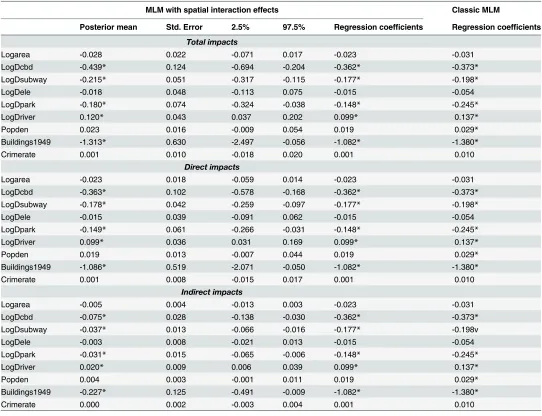
As for the magnitude of covariate effects, we should interpret them in terms of total, direct and indirect impacts [18].Table 3summarises these impact measures for each covariate sup-plemented with the estimated regression coefficients from the proposed method and from the classic MLM. The total or marginal impacts of each independent variable are larger than their coefficients due to a positive spatial interaction effect. As for interpreting the magnitude of these impacts, taking the example of the covariate effect of LogDcbd, if the proximity to CBD increases (or the distance to CBD decreases) by 1%, land prices will increase by 0.363% from a direct effect, and by 0.075% from an indirect effect, producing a total effect of 0.439% increase.

Table 2. Regression coefficients estimation results from the land parcel price data set.

MLM with spatial interaction effects Classic MLM

Posterior mean Std. Error 2.5% 97.5% Posterior mean Std. Error 2.5% 97.5%

Intercept 11.357* 0.958 9.448 13.248 13.627* 0.702 12.211 14.998

Logarea -0.023 0.018 -0.059 0.013 -0.031 0.019 -0.068 0.006

LogDcbd -0.362* 0.102 -0.576 -0.168 -0.373* 0.075 -0.520 -0.227

LogDsubway -0.177_* 0.042 -0.258 -0.097 -0.198_* 0.042 -0.278 -0.115

LogDele -0.015 0.039 -0.091 0.062 -0.054 0.038 -0.127 0.019

LogDpark -0.148* 0.061 -0.266 -0.031 -0.245* 0.056 -0.359 -0.136

LogDriver 0.099* 0.036 0.031 0.168 0.137* 0.036 0.069 0.206

Popden 0.019 0.013 -0.007 0.044 0.029_* 0.014 0.001 0.056

Buildings1949 -1.082* 0.518 -2.067 -0.050 -1.380* 0.426 -2.211 -0.544

Crimerate 0.001 0.008 -0.015 0.017 0.010 0.010 -0.010 0.029

Year04 -0.209* 0.056 -0.320 -0.104 -0.191* 0.056 -0.299 -0.083

Year05 -0.048 0.118 -0.281 0.188 -0.024 0.119 -0.259 0.216

Year06 -0.064 0.103 -0.272* 0.137 -0.077 0.105 -0.281 0.133

Year07 0.732* 0.114 0.507 0.955 0.736* 0.118 0.505 0.959

Year08 0.535* 0.127 0.288 0.775 0.564* 0.128 0.313 0.816

Year09 2.326* 0.217 1.904 2.747 2.187* 0.216 1.762 2.607

ρ 0.174* 0.036 0.104 0.246 NA NA NA NA

λ 0.760* 0.145 0.387 0.959 NA NA NA NA

σu2 0.052* 0.021 0.020 0.102 0.125* 0.030 0.075 0.192

σe2 0.574* 0.025 0.525 0.624 0.579* 0.026 0.530 0.633

*denotes statistically significant at 95% credible level or above.

Evaluating at the mean proximity to subway stations and the mean land price, the marginal value of decreasing the distance to nearest stations by 100 metres yields a 34.5 RMB total increase for per square metre land, which consists of a 27.8 RMB increase from direct impacts and 6.7 RMB increase from indirect impacts.

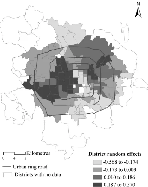
Contextual effects visualization. Fig 8maps the estimated posterior means of district level random effects from the proposed model. The breaking points correspond to the lower, median and upper quartiles of the district effects, with darker colours indicating stronger effects. Overall, there is a clear spatial pattern: high and low values of district effects clustering together respectively because of the significant and relatively large spatial autoregressive parameter observed (λ).

Table 3. The total, direct and indirect impacts of selected covariates using estimates from the proposed methodology.

MLM with spatial interaction effects Classic MLM

Posterior mean Std. Error 2.5% 97.5% Regression coefficients Regression coefficients

Total impacts

Logarea -0.028 0.022 -0.071 0.017 -0.023 -0.031

LogDcbd -0.439* 0.124 -0.694 -0.204 -0.362* -0.373*

LogDsubway -0.215_* 0.051 -0.317 -0.115 -0.177_* -0.198_*

LogDele -0.018 0.048 -0.113 0.075 -0.015 -0.054

LogDpark -0.180* 0.074 -0.324 -0.038 -0.148* -0.245*

LogDriver 0.120* 0.043 0.037 0.202 0.099* 0.137*

Popden 0.023 0.016 -0.009 0.054 0.019 0.029_*

Buildings1949 -1.313* 0.630 -2.497 -0.056 -1.082* -1.380*

Crimerate 0.001 0.010 -0.018 0.020 0.001 0.010

Direct impacts

Logarea -0.023 0.018 -0.059 0.014 -0.023 -0.031

LogDcbd -0.363* 0.102 -0.578 -0.168 -0.362* -0.373*

LogDsubway -0.178* 0.042 -0.259 -0.097 -0.177* -0.198*

LogDele -0.015 0.039 -0.091 0.062 -0.015 -0.054

LogDpark -0.149* 0.061 -0.266 -0.031 -0.148* -0.245*

LogDriver 0.099* 0.036 0.031 0.169 0.099* 0.137*

Popden 0.019 0.013 -0.007 0.044 0.019 0.029*

Buildings1949 -1.086* 0.519 -2.071 -0.050 -1.082* -1.380*

Crimerate 0.001 0.008 -0.015 0.017 0.001 0.010

Indirect impacts

Logarea -0.005 0.004 -0.013 0.003 -0.023 -0.031

LogDcbd -0.075* 0.028 -0.138 -0.030 -0.362* -0.373*

LogDsubway -0.037* 0.013 -0.066 -0.016 -0.177* -0.198v

LogDele -0.003 0.008 -0.021 0.013 -0.015 -0.054

LogDpark -0.031* 0.015 -0.065 -0.006 -0.148* -0.245*

LogDriver 0.020* 0.009 0.006 0.039 0.099* 0.137*

Popden 0.004 0.003 -0.001 0.011 0.019 0.029*

Buildings1949 -0.227* 0.125 -0.491 -0.009 -1.082* -1.380*

Crimerate 0.000 0.002 -0.003 0.004 0.001 0.010

The last two columns are the regression coefficients from the proposed method and from the classic MLM. *denotes statistically significant at 95% credible level or above.

From the map we can identify two main areas with large district effects. These are in the northeast and the western parts of urban areas in Beijing, which is in accordance with previous studies [24]. The northeastern area has been planned as a major urban sub-centre of Beijing and has a lot of large residential communities provided with sufficient supplementary commer-cial facilities such as large shopping malls and with many service-related job opportunities. The land use mix improves land values especially within the large residence-function orientated urban areas [26]. For the western areas (between the second and fourth ring roads), the cluster-ing of high land prices might be related to the concentration of jobs and educational facilities such as universities, high-quality primary and high schools.

For comparison,Fig 9maps the estimated posterior means of the district level random effects from the MLM, using the same breakpoints as inFig 8. The overall spatial pattern is more discrete than that inFig 8because the MLM assumes these district random effects to be independent of each other. In contrast, the proposed MLM with spatial interaction effects exploits the estimation of the random effects from the neighbouring districts to calculate the summary for a particular district, thus providing more smoothed estimates than the MLM. In addition, we test whether the district effects from the MLM are spatially dependent by using the Moran’s I statistic based on the spatial weights matrixM[15]. The resultant Moran coeffi-cient is 0.223 with a p-value equal to<0.001. This demonstrates the existence of positive spatial dependence in the estimated district effects from the MLM. It contradicts the core model assumption of independence of the higher level residuals.

Fig 8. The district level random effects from the proposed MLM with spatial interactions.

Conclusions

With the increasing availability of geographically hierarchical datasets, multilevel models are widely employed to examine the outcomes of interest measured at the lower and higher levels simultaneously. The purpose is to avoid the "ecological fallacy" when transferring relationships between variables at aggregate spatial scales to individuals, to avoid the "atomistic fallacy" where correlations between variables are investigated exclusively at the individual level without consideration to the context, to look for and to quantify contextual effects, and to provide bet-ter estimates of model paramebet-ters and their standard errors in the presence of such effects [27].

Despite being frequently applied to geographical data, the classic MLM is not really a spatial modelling technique as it does not consider the possibility of proximity effects between the units of analysis. It does not model spatial interaction effects and is incapable of distinguishing between contextual effects and spatial interaction effects. The consequence associated with this is that the contextual effects estimated by employing the MLM will be confounded with any spatial interaction effects. From the simulation study, where the data generating process con-sists of both the contextual effects and the positive spatial interaction effects at each spatial scale, we see that the MLM produces biased estimation for the covariate effects and for the two variance parameters. The implication for future empirical studies in which the classic MLM is chosen concerns the validity of the statistical inference on covariate effects especially for the estimated contextual effects, and of the interpretation on how important group dependence is in explaining the outcome variations of interest.

This paper provides an integrated spatial econometrics and multilevel methodological framework for modelling spatial data with a hierarchical structure, allowing for separation of

Fig 9. The district level random effects from the classic MLM.

the (horizontal) spatial interaction effect from the (vertical) group dependence effect. Using the proposed MLM with spatial interaction effects, we find significant spatial interactions among the residential land parcels and among the districts in Beijing, China. Given the prolif-eration of hierarchical spatial data and their extensive use in regional economics, health and environmental research, we anticipate that our approach could be useful in a wide range of applications. Though the method is illustrated using spatial data, the approach is also suitable to model hierarchical social network data where social network effects and contextual effects might simultaneously impact outcomes or behaviours of individuals [28].

We end this paper by discussing further elaborations to the proposed MLM with spatial interaction effects. In a way similar to a random slope multilevel model, a future model exten-sion would be to allow for spatially varying regresexten-sion coefficients across space. For example, regression coefficients for certain land parcel level covariates could vary across districts. This enables us to explore spatial heterogeneity in the covariate effects. Spatial heterogeneity in the covariate effects across higher level spatial units can be constructed by using a multivariate con-ditional autoregressive process [20,29]. This extension is our next step towards an integrated spatial and multilevel modelling technique.

Supporting Information

S1 Appendix. R code to implement the developed methodology.We provide the R code to implement the developed methodology. In addition, R scripts that demonstrate how to use the core function and reproduce the land price model results in the manuscript are provided. (ZIP)

S1 Dataset. The land price data set used in the empirical study. (CSV)

Acknowledgments

The authors gratefully thank the three referees and the academic editor for their time in provid-ing comments on an earlier version of the article. The first author greatly acknowledges the U. K. ESRC for funding his doctoral research.

Author Contributions

Conceived and designed the experiments: GD RH. Performed the experiments: GD RH JY. Analyzed the data: GD JY. Contributed reagents/materials/analysis tools: GD RH KJ JY. Wrote the paper: GD RH KJ.

References

1. Goldstein H (2003) Multilevel statistical methods.( 3rd ed.). London: Arnold.

2. Jones K (1991) Specifying and estimating multi-level models for geographical research. T I Brit Geogr 16: 148–159.

3. Jones K, Duncan C (1995) Individuals and their ecologies: analysing the geography of chronic illness within a multilevel modelling framework. Health Place 1: 27_–40.

4. Corrado L, Fingleton B (2012) Where is the economics in spatial econometrics. J Regional Sci 52: 210–239.

5. Baltagi BH, Fingleton B, Pirotte A (2014) Spatial lag models with nested random effects: an instrumen-tal variable procedure with an application to English house prices. J Urban Econ 80: 76–86.

7. Savitz NV, Raudenbush SW (2009) Exploiting spatial dependence to improve measurement of neigh-bourhood social processes. Sociol Methodol 5: 151–182.

8. Dong GP, Harris R (In press) Spatial autoregressive models for geographically hierarchical data struc-tures. Geogr Anal, doi:10.1111/gean.12049PMID:25684791

9. Langford IH, Leyland AH, Rasbash J, Goldstein H (1999) Multilevel modelling of the geographical distri-butions of diseases. J Roy Stat Soc C-App 48: 253–268. PMID:12294883

10. Browne WJ, Goldstein H, Rasbash J (2001) Multiple membership multiple classification (MCMC) mod-els. Stat Model 1: 103–124.

11. Tranmer M, Steel D, Browne WJ (2014) Multiple-membership multiple-classification models for social network and group dependence. J Roy Stat Soc A Sta 177: 439–455. PMID:25598585

12. Arcaya M, Brewster M, Zigler CM, Subramanian SV (2012) Area variations in health: a spatial multilevel modeling approach. Health Place 18: 824_–831. doi:10.1016/j.healthplace.2012.03.010PMID: 22522099

13. Chaix B, Merlo J, Chauvin P (2005) Comparison of a spatial approach with the multilevel approach for investigating place effects on health: the example of healthcare utilization in France. J Epidemiol Com-mun H 59: 517–526.

14. Anselin L (1988) Spatial Econometrics: Methods and Models. Dordrecht: Kluwer Academic Publishers.

15. Cliff A, Ord JK (1981) Spatial Processes: Models and Applications. London: Pion.

16. Griffith DA (1988) Advanced spatial statistics: special topics in the exploration of quantitative spatial data series. Dordrecht: Kluwer.

17. Haining R (2003) Spatial data analysis: theory and practice. Cambridge: Cambridge University Press. 18. LeSage JP, Pace RK (2009) Introduction to Spatial Econometrics. Boca Raton: Chapman and Hall/

CRC.

19. Cressie N (1993) Statistics for Spatial Data, Revised edition. New York: Wiley.

20. Banerjee S, Carlin BP, Gelfand AE (2004) Hierarchical Modelling and Analysis for Spatial Data. Boca Raton: Chapman and Hall/CRC.

21. Lee D (2011) A comparison of conditional autoregressive models used in Bayesian disease mapping. Spatial and Spatio-temporal Epidemiology 2: 79–89. doi:10.1016/j.sste.2011.03.001PMID:22749587 22. Griffith DA (2005) Effective geographic sample size in the presence of spatial autoregression. Ann

Assoc Am Geogr 95: 740–760.

23. Zheng SQ, Kahn ME (2008) Land and residential property markets in a booming economy: New evi-dence from Beijing. J Urban Econ 63: 743_–757.

24. Dong GP, Zhang WZ, Wu WJ, Guo TY (2011) Spatial heterogeneity in determinants of residential land prices: simulation and prediction. Acta Geographica Sinica 66: 750–760.

25. Harris R, Dong GP, Zhang WZ (2013) Using contextualised geographically weighted regression to model the spatial heterogeneity of land prices in Beijing, China. Transaction in GIS 17: 901–919. 26. Cheshire P, Sheppard S (1995) On the price of land and the value of amenities. Economica 62: 247_–

267.

27. Subramanian SV, Jones K, Duncan C (2003) Multilevel methods for public health research. In Kawachi I., & Berkman L. F. (Eds.), Neighbourhoods and health (pp.65–111). New York: Oxford University Press.

28. Laszkiewicz E, Dong GP, Harris R (2014) The effect of omitted spatial effects and social dependence in the modelling of household expenditure for fruits and vegetables. Comparative Economic Research 17: 155–172.