White Rose Research Online URL for this paper:
http://eprints.whiterose.ac.uk/92411/
Version: Accepted Version
Article:
Levinsen, JF, Khvorostovsky, K, Ticconi, F et al. (12 more authors) (2015) ESA ice sheet
CCI: derivation of the optimal method for surface elevation change detection of the
Greenland ice sheet - round robin results. International Journal of Remote Sensing, 36 (2).
pp. 551-573. ISSN 0143-1161
https://doi.org/10.1080/01431161.2014.999385
[email protected] https://eprints.whiterose.ac.uk/ Reuse
Unless indicated otherwise, fulltext items are protected by copyright with all rights reserved. The copyright exception in section 29 of the Copyright, Designs and Patents Act 1988 allows the making of a single copy solely for the purpose of non-commercial research or private study within the limits of fair dealing. The publisher or other rights-holder may allow further reproduction and re-use of this version - refer to the White Rose Research Online record for this item. Where records identify the publisher as the copyright holder, users can verify any specific terms of use on the publisher’s website.
Takedown
If you consider content in White Rose Research Online to be in breach of UK law, please notify us by
To appear in theInternational Journal of Remote Sensing
Vol. 00, No. 00, Month 20XX, 1–22
ESA Ice Sheets CCI: Derivation of the optimal method for surface
elevation change detection of the Greenland Ice Sheet – Round
Robin results
J.F. Levinsena∗, K. Khvorostovskyb, F. Ticconic,d, A. Shepherdc, R. Forsberga, L.S.
Sørensena, A. Muire, N. Pief, D. Feliksonf, T. Flamentc, R. Hurkmansg, G. Moholdth, B.
Gunteri,j, R.C. Lindenberghi, M. Kleinherenbrinki
aDTU Space, National Space Institute, Technical University of Denmark, Elektrovej,
Building 327 + 328, 2800 Kongens Lyngby, Denmark;
bNN, Nansen Environmental and Remote Sensing Center, Thormøhlens gate 47, 5006
Bergen, Norway;
cSchool of Earth and Environment, University of Leeds, Leeds LS2 9JT, UK;
dEUMETSAT, Remote Sensing and Product Unit, Eumetsat Allee 1, 64295 Darmstadt,
Germany;
eUniversity College London, Gower Street, London, WC1E 6BT, UK;
f
University of Texas, Center for Space Research, 3925 West Braker Lane, Suite 200,
Austin, Texas 78759-5321, USA;
gBristol Glaciology Centre, School of Geographical Sciences, University of Bristol,
University Road, Bristol, BS8 1SS, UK;
hScripps Institution of Oceanography, 9500 Gilman Drive, La Jolla, 92093-0225, USA; iDepartment of Geoscience & Remote Sensing, Delft University of Technology, 2600 GA
Delft, the Netherlands;
j
School of Aerospace Engineering, Georgia Institute of Technology, 270 Ferst Drive, Atlanta, GA 30332-0150, USA
(Received:)
For more than two decades, radar altimetry missions have provided continuous ele-vation estimates of the Greenland Ice Sheet (GrIS). Here, we propose a method for using such data to estimate ice sheet-wide surface elevation changes (SEC). The final dataset will be based on observations acquired with the European Space Agency’s En-visat, ERS-1 and -2, CryoSat-2, and, in the longer term, Sentinel-3 satellites. In order to find the best-performing method, an inter-comparison exercise has been carried out in which the scientific community was asked to provide their best SEC estimate as well as a feedback sheet describing the applied method. Due to the hitherto few radar-based SEC analyses as well as the higher accuracy of laser data, the participants were asked to use either Envisat radar or ICESat (Ice, Cloud, and land Elevation Satel-lite) laser altimetry over the Jakobshavn Isbræ drainage basin. The submissions were validated against airborne laser-scanner data, and inter-comparisons were carried out to analyze the potential in the applied methods and whether the two altimeters were capable of resolving the same signal. The analyses found great potential in the ap-plied repeat-track and cross-over techniques, and, for the first time over Greenland, that repeat-track analyses from radar altimetry agreed well with laser data. Since topography-related errors can be neglected in cross-over analyses, it is expected that the most accurate, ice sheet-wide SEC estimates are obtained by combining the
over and repeat-track techniques. It is thus possible to exploit the high accuracy of the former and the large spatial data coverage of the latter. Based on CryoSat’s different operation modes, and the increased spatial and temporal data coverage, this shows good potential for a future inclusion of CryoSat-2 and Sentinel-3 data to continuously obtain accurate SEC estimates both in the interior and margin ice sheet.
Keywords:Surface elevation changes; Greenland; cross-over analyses; repeat-track analyses; laser and radar altimetry
1. Introduction
As the climate is changing, a need has arisen for scientists and space agencies across the globe to combine their efforts into establishing long-term data records to observe the changes. This has led the European Space Agency to establish the Climate Change Initiative (ESA CCI) in which 13 Essential Climate Variables are analyzed, such as sea ice, ozone, fire, and ice sheets (ESA 2011a). This work is part of the Ice Sheets CCI for which the focus area is the Greenland Ice Sheet (GrIS). The motivation is an increased mass loss, e.g. demonstrated by Zwally et al. (2011) who used laser and radar altimetry and found an increase of 164±5 Gt yr−1
from 1992–2002 to 2003–2007. Shepherd et al. (2012) compared mass balance estimates from the input-output method, laser altimetry, and gravimetry, and for reconciled estimates for 1992–2000 and 2000–2011, respectively, found that the mass loss rose from −51±65 Gt yr−1
to−211±37 Gt yr−1
.
In order to increase our understanding of the changes, the goal of this work is to develop a method for creating ice sheet-wide maps of surface elevation changes (SEC) based on ESA radar altimetry from ERS, Envisat, CryoSat-2 and Sentinel-3. This will enable the construction of time series running from 1992 until present date. In order to find the optimal method for the respective SEC production, a broad collaboration between relevant cryospheric and climate-related research groups is carried out. This is done in a so-called Round Robin (RR) exercise where members of the scientific community are contacted and encouraged to submit their best estimate as well as an in-depth description of the applied method. Here, we present the outcome of this exercise. The submitted results are inter-compared and validated against airborne laser-scanner data, and the resulting conclusions form the basis for the final GrIS SEC production.
2. Surface elevation change studies from altimetry
Observations from both laser (LA) and radar (RA) altimetry are used in several SEC studies of the ice sheets, e.g. by Zwally et al. (2005, 2011); Sørensen et al. (2011); Flament and R´emy (2012); Khvorostovsky (2012); Helm et al. (2014). Com-mon approaches are the repeat-track (RT) and cross-over (XO) techniques where measurements along repeated ground-tracks or in XO locations between ascending and descending satellite passes are explored. The different methods are described by Slobbe et al. (2008); Moholdt et al. (2010); Gunter et al. (2014).
errors. Nghiem et al. (2005) found penetration depths to exceed 1 m for Ku-band data over Greenland, while Forsberg et al. (2002), for C-band data, found 15– 20 m in the dry accumulation zone near the Geikie Plateau, which decreased to zero towards lower altitudes. Such errors are not found in LA as the echoes reflect directly off the surface (Brenner et al. 1983, 2007; Ridley and Partington 1988; Bamber 1994). This explains the findings by Brenner et al. (2007) in a comparison of ICESat and Envisat surface elevations over Greenland and Antarctica: They found a laser elevation precision of 14 – 50 cm depending on the surface slope, and elevation differences ranging from 9±52 cm for slopes less than 0.1◦
to 2.7±26 m for slopes up to 0.9◦
. The effect therefore varies when moving from the sloping, often specular coastal margin to the smoother interior with a smaller surface roughness (Legresy et al. 2005; R´emy et al. 2012; Sørensen et al. 2014).
Slope-related errors can be attributed to two things: For RA, the large footprint means that the reflecting point over a sloping surface rarely coincides with nadir but rather somewhere up-slope. In this case, one can either correct the range mea-surement to the sub-satellite point, or the elevation meamea-surement by e.g. adding a term based on the surface slope. For a 1◦
surface slope and a satellite altitude of 800 km, this error can shift measurement locations up to 14 km from nadir and introduce a vertical offset of approximately 120 m (Brenner et al. 1983; Fu and Cazenave 2001; Hurkmans et al. 2012).
In RT analyses, an error results from the footprint rarely being exactly repeat. It is, however, larger for RA as e.g. ICESat is capable of performing off-nadir maneu-vers to better repeat previous ground-tracks (Schutz et al. 2005). In any case, the local surface topography in-between ground-tracks must be considered. This can be done by estimating the slope bias from the distance between ground-tracks as well as the surface slope between them, the latter derived from an external Digital Elevation Model (DEM) (Slobbe et al. 2008).
RT analyses from RA therefore suffer from two types of slope-induced errors, which significantly increase data errors. Advantages are thus given to LA-based analyses, or to XO studies where measurements in overlapping ground-track loca-tions are explored; hence, effects from the local topography can be ignored.
3. The Round Robin exercise
The Ice Sheets CCI RR was announced through personal invitations, postings on the CCI web-site (www.esa-icesheets-cci.org/), and on the e-mailing list for snow and ice related research, CRYOLIST (www.cryolist.org/). In order to establish a basis for inter-comparing the results, the participants were given an observation area and instructions on which data to use. They were asked to submit their best SEC estimate, errors, and a feedback sheet describing pre- and post-processing steps, estimation specifications, computational time, etc. This allowed for inter-comparing the applied approaches.
The focus area was the Jakobshavn Isbræ drainage basin (68–71◦
N; 39–52◦
W), and the participants could use either ICESat or Envisat data. Laser data were included due to their high elevation accuracy and the sparsity of recent RA SEC studies of the GrIS. If a DEM was needed, the Greenland Ice Mapping Project (GIMP) model by Howat et al. (2014), originally posted at a 90 m resolution, was recommended.
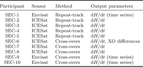
Table 1. Sensors and methods used for the SEC production as well as the final data parameters submitted by the Round Robin participants.
Participant Sensor Method Output parameters
SEC-1 Envisat Repeat-track dH/dt(time series)
SEC-2 ICESat Repeat-track dH/dt
SEC-3 ICESat Repeat-track dH/dt
SEC-4 ICESat Repeat-track dH/dt
SEC-5 ICESat Repeat-track dH/dt
SEC-6 ICESat Cross-overs dH/dt, XO differences
SEC-7 ICESat Cross-overs dH/dt
SEC-8 ICESat Cross-overs dH/dt
SEC-9 Envisat Cross-overs dH/dt(time series)
SEC-10 Envisat Cross-overs dH/dt(time series)
method used by the participants as well as the submitted output parameters; a more elaborate description of the methodologies is given in Section 3.2 and by Scharrer et al. (2013). In order to anonymize the results, the participants are re-ferred to as SEC-1, SEC-2,. . . , SEC-10, the order in which they are named being random. Three participants used Envisat data and the remaining seven ICESat. Of these, five groups applied the XO technique and the remaining five RT.
Some groups submitted both elevation time series and SEC estimates. In the for-mer, a formation of time series is first made, e.g. one for each grid cell, after which typically linear least-squares regression is used to fit a trend to the surface eleva-tions. The direct estimates are made when fitting a trend to elevation differences (dH) vs. the temporal difference between the data acquisition times (dt).
The submissions are validated against airborne laser-scanner data acquired with NASA’s Airborne Topographic Mapper (ATM). Such data are used due to their high accuracy and spatial data coverage (Krabill et al. 2002). Finally, a number of the submissions are inter-compared to analyze the applied techniques and sensors. Thus, analyses of cross-over vs. repeat-track results and radar vs. laser altimetry are carried out, to test the validity of the applied methods and investigate the performance of RA relative to LA. On the basis of the extensive amount of sub-missions across sensors and methods, the final conclusions form the basis for the optimal RA SEC solution for the GrIS.
3.1. Temporal extent and spatial resolution
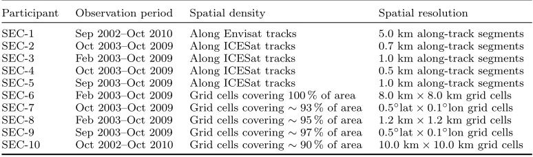
[image:5.612.170.411.80.194.2]Table 2. Observation period, spatial density, and spatial resolution of the Round Robin SEC products.
Participant Observation period Spatial density Spatial resolution
SEC-1 Sep 2002–Oct 2010 Along Envisat tracks 5.0 km along-track segments
SEC-2 Oct 2003–Oct 2009 Along ICESat tracks 0.7 km along-track segments
SEC-3 Feb 2003–Oct 2009 Along ICESat tracks 1.0 km along-track segments
SEC-4 Oct 2003–Oct 2009 Along ICESat tracks 0.5 km along-track segments
SEC-5 Sep 2003–Oct 2009 Along ICESat tracks 1.0 km along-track segments
SEC-6 Feb 2003–Oct 2009 Grid cells covering 100 % of area 8.0 km×8.0 km grid cells
SEC-7 Oct 2003–Oct 2009 Grid cells covering∼93 % of area 0.5◦lat×0.1◦lon grid cells
SEC-8 Feb 2003–Oct 2009 Grid cells covering∼95 % of area 1.2 km×1.2 km grid cells
SEC-9 Sep 2003–Oct 2009 Grid cells covering∼97 % of area 0.5◦lat×0.1◦lon grid cells
SEC-10 Oct 2002–Oct 2010 Grid cells covering∼90 % of area 10.0 km×10.0 km grid cells
3.2. Methodology
The feedback sheets reveal that the ICESat data processing is very similar, with common data rejection criteria for the saturation index, the incident beam co-elevation angle, the return signal’s gain value, and the return waveform only having one peak. Table 3 lists the details of the RR product generation, and it is found that all RT groups apply linear least-square (LSq) techniques, namely weighted, unweighted and multi-variate LSq. SEC-2 fits a plane to near repeat-tracks, solv-ing for both the surface slope and dH/dt signal. SEC-3 solves for both dH/dx, dH/dy, and dH/dt whereas SEC-1 also solves for the waveform parameters, i.e. backscatter, trailing edge slope, and leading edge width (Legresy et al. 2005). Only one group relocates the RA points: SEC-1 who uses a Point of Closest Approach (POCA) method (Gray et al. 2013; Hawley et al. 2009). The errors from SEC-1, SEC-3, and SEC-4 are given as the standard error of the LSq fit, SEC-2 uses the one from the plane fitting and SEC-5 that from the unweighted LSq covariance matrix combined with the RMS of the elevation estimation residuals within each along-track segment.
The SEC estimation is carried out similarly for SEC-7, SEC-9, and SEC-10, who apply a linear-sinusoidal fit to time series of elevation differences. SEC-9 filtered observations with noise levels of the waveforms exceeding five counts. SEC-6 sub-mitted the median dH/dt signal from all values within each grid cell, whereas SEC-8 applies an unweighted LSq fit in which data errors are included through data covariance matrices (e.g. Gunter et al. (2014); Khvorostovsky (2012); Zwally et al. (2005)). The error estimates from SEC-7, SEC-9, and SEC-10 are given as the standard error of the time series trends, while SEC-6’s errors represent the standard deviation (STD) of the SEC values in each grid cell. Finally, SEC-9 and SEC-10 have corrected the SEC estimates for backscatter effects when the corre-lation between elevation differences (dH) and changes in the received backscatter power (dσ0) is either positive or exceeds 0.5, respectively. The relation between the two is given by dH = dH−dσ0×(dH/dσ0) (Arthern 1997; Khvorostovsky 2012). An additional correction applied by SEC-9 is that for the leading edge width and trailing edge slope.
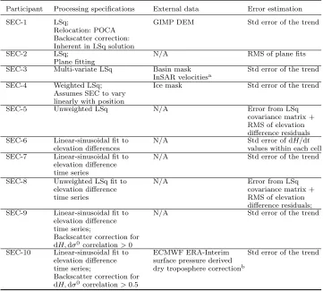
[image:6.612.97.484.61.175.2]Table 3. Overview of the repeat-track and cross-over methodologies used by the RR participants. ”LSq” abbreviates linear least-squares regression and ”POCA” the Point Of Closest Approach method.
Participant Processing specifications External data Error estimation
SEC-1 LSq;
Relocation: POCA Backscatter correction: Inherent in LSq solution
GIMP DEM Std error of the trend
SEC-2 LSq;
Plane fitting
N/A RMS of plane fits
SEC-3 Multi-variate LSq Basin mask
InSAR velocitiesa Std error of the trend
SEC-4 Weighted LSq;
Assumes SEC to vary linearly with position
Ice mask Std error of the trend
SEC-5 Unweighted LSq N/A Error from LSq
covariance matrix + RMS of elevation difference residuals
SEC-6 Linear-sinusoidal fit to
elevation differences
N/A Std error of dH/dt
values within each cell
SEC-7 Linear-sinusoidal fit to
elevation difference time series
N/A Std error of the trend
SEC-8 Unweighted LSq fit to
elevation difference time series
N/A Error from LSq
covariance matrix + RMS of elevation difference residuals;
SEC-9 Linear-sinusoidal fit to
elevation difference time series;
Backscatter correction for dH,dσ0
correlation>0
N/A Std error of the trend
SEC-10 Linear-sinusoidal fit to
elevation difference time series;
Backscatter correction for dH,dσ0
correlation>0.5
ECMWF ERA-Interim surface pressure derived dry troposphere correctionb
Std error of the trend
a
Ice velocities are obtained from Joughin et al. (2010). b
The correction for the dry troposphere is described in ESA (2011b).
3.3. Validation
The RR results are validated against SEC trends derived from ATM data. The campaigns are carried out yearly, except for in 2004, in the months April, May, and August. In order to ensure temporal consistency, two separate trends are derived for 2003–2009 and 2002–2010, respectively. The focus area is the main trunk of Jakobshavn (68.5–70◦
N; 47–50.5◦
W) where the largest surface changes are observed (Joughin et al. 2014; Liu et al. 2012; Nielsen et al. 2013). The ATM trends are derived by fitting a linear trend as well as cyclic terms to the observations. In order to make a proper ground truth, only values based on a minimum of three observation periods are used.
The validation is carried out by subtracting the ATM dH/dttrend from the RR values. This is done by, for each RR point, finding all available ATM observations within a polygon surrounding the point. The size of the polygon is determined by the spatial resolution used in the respective submission (Table 2). The given ATM values are averaged to find the mean, which is subtracted from the RR value to give dH/dt∆= dH/dtRR−dH/dtATM. Finally, the mean and STD of dH/dt∆are
[image:7.612.111.472.79.404.2]−50 −45 −40 68 68.5 69 69.5 70 70.5 71
Longitude (°)
Latitude (
°
)
SEC−1
−50 −45 −40
68 68.5 69 69.5 70 70.5 71
Longitude (°)
Latitude (
°
)
SEC−2
−50 −45 −40
68 68.5 69 69.5 70 70.5 71
Longitude (°)
Latitude (
°
)
SEC−3
−50 −45 −40
68 68.5 69 69.5 70 70.5 71
Longitude (°)
Latitude (
°
)
SEC−4
−50 −45 −40
68 68.5 69 69.5 70 70.5 71
Longitude (°)
Latitude (
°
)
SEC−5
−50 −45 −40
68 68.5 69 69.5 70 70.5 71
Longitude (°)
Latitude (
°
)
SEC−6
−50 −45 −40
68 68.5 69 69.5 70 70.5 71
Longitude (°)
Latitude (
°
)
SEC−7
−50 −45 −40
68 68.5 69 69.5 70 70.5 71
Longitude (°)
Latitude (
°
)
SEC−8
−50 −45 −40
68 68.5 69 69.5 70 70.5 71
Longitude (°)
Latitude (
°
)
SEC−9
−50 −45 −40
68 68.5 69 69.5 70 70.5 71
Longitude (°)
Latitude (
°
)
SEC−10
(m yr−1)
−6 −5 −4 −3 −2 −1 0 1 2 3
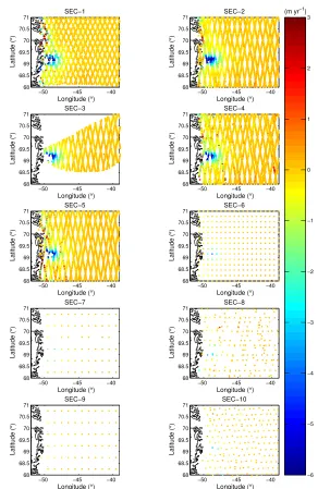
Figure 1. Surface elevation change estimates derived using repeat-tracks (participants SEC-1 to SEC-5) and cross-overs (SEC-6 to SEC-10).
such as the along-track segments used in RT analyses, which are confined to the ground-track and limited by the altimeter’s footprint. For larger spatial resolutions, however, correspondingly larger variations in the SEC signal may occur thereby affecting the statistics.
4. Results
[image:8.612.143.435.46.495.2]−50 −45 −40 68 68.5 69 69.5 70 70.5 71
Longitude (°)
Latitude (
°
)
SEC−1
−50 −45 −40
68 68.5 69 69.5 70 70.5 71
Longitude (°)
Latitude (
°
)
SEC−2
−50 −45 −40
68 68.5 69 69.5 70 70.5 71
Longitude (°)
Latitude (
°
)
SEC−3
−50 −45 −40
68 68.5 69 69.5 70 70.5 71
Longitude (°)
Latitude (
°
)
SEC−4
−50 −45 −40
68 68.5 69 69.5 70 70.5 71
Longitude (°)
Latitude (
°
)
SEC−5
−50 −45 −40
68 68.5 69 69.5 70 70.5 71
Longitude (°)
Latitude (
°
)
SEC−6
−50 −45 −40
68 68.5 69 69.5 70 70.5 71
Longitude (°)
Latitude (
°
)
SEC−7
−50 −45 −40
68 68.5 69 69.5 70 70.5 71
Longitude (°)
Latitude (
°
)
SEC−8
−50 −45 −40
68 68.5 69 69.5 70 70.5 71
Longitude (°)
Latitude (
°
)
SEC−9
−50 −45 −40
68 68.5 69 69.5 70 70.5 71
Longitude (°)
Latitude (
°
)
SEC−10
(m yr−1)
0 0.25 0.5 0.75 1 1.25 1.5
Figure 2. Surface elevation change errors from repeat-track (participants SEC-1 to SEC-5) and cross-over (SEC-6 to SEC-10) analyses.
4.1. The Round Robin exercise
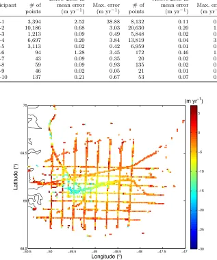
Figures 1 and 2 show the participants’ elevation change estimates and correspond-ing errors. The results are presented accordcorrespond-ing to the use of RT and XO, respec-tively. The errors are derived in various ways, such as from the standard error of the trend, or by including covariance matrices. Therefore, the values are not directly comparable. They do, however, provide important information on the accuracy of the different methods and thus are included after all.
[image:9.612.144.435.44.493.2]show a larger thinning.
The associated errors decrease with an increasing elevation and are near-zero in the interior ice sheet. Therefore, the errors are described relative to their re-spective altitude, i.e. for locations above and below 2000 m (Table 4). Where no elevations are submitted, the GIMP DEM is used as a reference. For RT measure-ments below 2000 m, the LA results from SEC-2 and SEC-4 reveal maximum errors of 3 and 3.8 m yr−1
, respectively, while the values from SEC-3 and SEC-5 reach approximately 0.5 m yr−1
. SEC-1’s RA errors are larger and reach 39 m yr−1
. For measurements above 2000 m, the errors generally decrease due to the smoother surface exposed to smaller changes (Sørensen et al. 2011). Thus, SEC-1’s errors have decreased to a maximum of 0.9 m yr−1
, SEC-2’s to 1.9 m yr−1
, SEC-3’s to 0.2 m yr−1
, and SEC-5’s to 0.1 m yr−1
. The maximum error from SEC-4 is similar for both areas although more values are closer to zero (99% less than 1 m yr−1
over high elevation area against 97% at lower elevations).
Based on the above, SEC-1’s Envisat results are particularly interesting as they illustrate the possibility of using RA to observe surface changes even along the coastal margin where surface topography, due to high slopes and undulations, and penetration of the radar echoes distort the measurements. The results contain the largest errors however still provide an important insight into the surface changes. Additional differences between the measured SEC signals from RA and LA result from Envisat’s footprint preventing it from resolving small ice streams, the fact that the satellite cannot be pointed cross-track to ensure precise repeat-tracks, as well as the ICESat observation period being shorter by two years.
The XO results, SEC-6 to SEC-10, do not fully resolve the large thinning observed along the drainage basin and coastal margin using RT. This can be explained by the XO estimates being found by gridding the observations into cells, thereby losing part of the SEC signal due to an applied smoothing. As the RR participants have used differently-sized grid cells, observations from the same sensor do not agree in space; the only overlap is found for SEC-7 and SEC-9 due to the submissions coming from the same research institution. Interior dH/dtestimates agree well for the two sensors thereby illustrating the capabilities in this region regardless of the applied method and type of altimeter. The data errors (Table 4) for LA measurements below 2000 m reach a maximum of 3.5 m yr−1
for SEC-6, 0.4 m yr−1
for SEC-7, and 0.9 m yr−1
for SEC-8. The maximum errors of the radar-based submissions are 0.1 m yr−1
and 0.7 m yr−1
, respectively. As was observed using RT, estimates over higher elevations have smaller errors: SEC-6’s errors have decreased to 1.5 m yr−1
while those for SEC-7 and SEC-8 decreased to 0.1 and 0.6 m yr−1
. The RA errors are 0.0 m yr−1
for SEC-9 and 0.4 m yr−1
for SEC-10, respectively.
When comparing the values estimated with a similar method (column 4, Table 3), i.e. SEC-1, 3, 4, 7, 9, and SEC-10, giving the standard error of the trend, it is clear that the XO errors are typically lower. The reason for SEC-6 deviating from this is the estimation of the standard error of the dH/dtvalues instead. The lower XO errors indicate that such analyses produce the highest accuracy as slope effects from the local topography can be ignored. The method does, however, for RA require an initial slope-correction of data. Because of the spatial distribution of ground-tracks, XO points are limited in space, particularly along the coastal margin. The opposite is found with RT, which have a high spatial coverage however a smaller accuracy due to the lack of exact repeat ground-tracks.
In the following, results from SEC-7 and SEC-9 are given for the validation exercise; they are, however, not considered in detail neither here, nor in the inter-comparison. This is due to the size of the grid cells (0.5◦
lat ×0.1◦
ap-Table 4. Mean and maximum errors for repeat-track (SEC-1 to SEC-5) and cross-over (SEC-6 to SEC-10) analyses.
Below 2000 m Above 2000 m
Participant # of mean error Max. error # of mean error Max. error
points (m yr−1) (m yr−1) points (m yr−1) (m yr−1)
SEC-1 3,394 2.52 38.88 8,132 0.11 0.89
SEC-2 10,186 0.68 3.03 20,630 0.20 1.86
SEC-3 1,213 0.09 0.49 5,848 0.02 0.24
SEC-4 6,697 0.20 3.84 13,819 0.04 3.83
SEC-5 3,113 0.02 0.42 6,959 0.01 0.06
SEC-6 94 1.28 3.45 172 0.46 1.51
SEC-7 43 0.09 0.35 20 0.02 0.05
SEC-8 59 0.09 0.93 135 0.02 0.55
SEC-9 46 0.02 0.05 21 0.01 0.02
SEC-10 137 0.21 0.67 53 0.07 0.44
−50.5 −50 −49.5 −49 −48.5 −48 −47.5 −47
68.5 69 69.5 70
Longitude (°)
Latitude (
°
)
(m yr−1)
−30 −25 −20 −15 −10 −5 0 5
Figure 3. Validation data: Surface elevation changes derived from 2003–2009 ATM data. As the ATM flights largely cover the same flight lines, the 2002-2010 trend (not shown) is given along the same coordi-nates.
proximately 50 km ×50 km) relative to the respective footprint sizes: The spatial resolution cannot accurately reproduce the changes visible with neither sensor.
4.2. Validation with airborne laser-scanner data
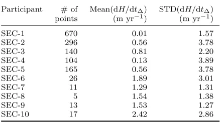
Validation is carried out with ATM data. Two SEC trends are derived for 2003– 2009 and 2002–2010, respectively; Figure 3 provides an example of the former. The mean and STD of the RR minus ATM SEC trends, dH/dt∆, are estimated
(Table 5). Due to the observation area being confined to the lowest part of the glacier and consequently the relatively small data sampling, particularly for XO measurements, the validation is not split up relative to the altitude.
[image:11.612.116.465.73.204.2] [image:11.612.133.450.83.462.2]the ICESat footprint. For SEC-1, whose results are based on Envisat RA and a spatial resolution of 5 km×5 km, the agreement is quite remarkable: This dataset has the smallest mean and STD of all RT measurements, namely 0.01 m yr−1
and 1.57 m yr−1
, respectively. The statistics are, undoubtedly, affected by the highest amount of validation points. However, the validity of SEC-1’s results is further confirmed in an inter-comparison below where scatter plots of LA and RA RT measurements reveal a coefficient of determination, R2, of 0.84. Both results confirm the capability of using RA data to resolve SEC estimates even in margin regions of the ice sheet.
In spite of the low RT mean values, the STD are generally higher than for XO. A possible explanation is that the validation points used for the RT comparison are located close to and along the coastal margin whereas those from XO typically have only a few observations in this region and most at high altitudes. As the margin region is subject to the largest surface changes, and a varying surface topography means that these patterns can change even within hundreds of meters (Levinsen et al. 2013), this can explain the relatively high RT STD.
This topographic difference also clarifies the smaller STD for XO measurements. Their respective means are generally higher, which is a result of the different RR SEC routines as well as the typically larger grid cells. The latter may complicate the process of obtaining agreeing ATM and RR results as any variations in the dH/dt trends are smoothed out in the averaging. The typically larger spatial resolutions in XO analyses reduce the number of validation points and increase the mean difference, namely from 0.41 m yr−1
for RT to 1.73 m yr−1
to XO. Therefore, when considering the XO results, it should be noted that the average number of observations for the comparison is 14 against 275 for the RT analyses.
The higher mean values are exactly observed for the remaining XO observations where SEC-6 has applied a spatial resolution of 8 km×8 km while that for SEC-7 and -9 is as large as 50 km×50 km. SEC-8 have the smallest cells and thus should reveal the optimal agreement with ATM data; however, given such a small spatial resolution, only five validation points are available, and hence the respective mean and STD are not believed to fully represent the dataset.
SEC-10 has the largest mean of 2.42 m yr−1
; the STD is 2.86 m yr−1
, i.e. second-highest after SEC-6. Similarly to SEC-1, the work is based on Envisat data. How-ever, although the size of the grid cells agree well with the RA footprint, no relo-cation of the estimation points has been carried out. This introduces errors when comparing with a laser-based dataset and hence explains the large offset.
As mentioned above, SEC-6 has the highest XO STD of 3.01 m yr−1
. Cf. Table 4, the dataset also has large errors; see the Discussion for more details on the reason.
Based on the above, the validation has shown the following:
• RT measurements provide the best validation results with near-zero means. This supports the application of a high spatial resolution and the exploitation of the large data coverage to be achieved with RT; both contribute to a high agreement with validation data.
• RT measurements are, however, subject to larger STD due to more of the observations being located at lower altitudes, where the SEC trends can vary greatly within small distances.
Table 5. Results from the validation of the Round Robin data sets using dH/dttrends derived from ATM data. The search radius used for overlapping grid cells is given by the spatial resolution of the respective submissions, just as well as the temporal coverage of the validation trends corre-sponds to that of the submissions (Table 2). dH/dt∆gives the dH/dtdifference between the Round Robin and ATM values, and the mean and STD hereof are presented.
Participant # of Mean(dH/dt∆) STD(dH/dt∆)
points (m yr−1) (m yr−1)
SEC-1 670 0.01 1.57
SEC-2 296 0.56 3.78
SEC-3 140 0.81 2.20
SEC-4 104 0.13 3.89
SEC-5 165 0.56 3.78
SEC-6 26 1.89 3.01
SEC-7 11 1.29 1.31
SEC-8 5 1.54 1.38
SEC-9 13 1.53 1.27
SEC-10 17 2.42 2.86
• Validation points for XO measurements are few in space, which biases the statistics. This is due to the larger grid cells in which parts of the SEC signal is lost due to smoothing of the observations. The result is generally higher mean differences.
4.3. Inter-comparison of Round Robin results
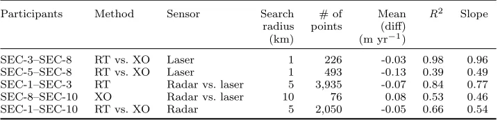
In order to thoroughly analyse the applied methods, a number of inter-comparisons are made. As before, only observations within similar spatial domains are com-pared. This is achieved by using search radii based on the spatial resolutions of the datasets in question. The given methods are then assessed by finding overlapping estimation points and differencing the SEC values herein (“diff”). The mean and root-mean-square-errors (RMSE) of these differences are calculated, and scatter plots are used for estimating the coefficient of determination and the slope of the regression (Figure 4 and Table 6).
The following analyses are carried out:
(1) Laser: Repeat-track vs. cross-overs - SEC-3 vs. SEC-8
The results from SEC-3 proved very accurate, the spatial resolutions are similar, and both datasets cover the period Feb. 2003–Oct. 2009. This analysis opens to testing the capabilities for ICESat change detection using XO. (2) Laser: Repeat-track vs. cross-overs - SEC-5 vs. SEC-8
The observations from SEC-5 span Sep. 2003–Oct. 2009, i.e. one summer less than SEC-8. The datasets do, however, have similar spatial resolutions. (3) RT: Laser vs. radar altimetry - SEC-1 vs. SEC-3
Both datasets proved highly accurate in the validation. (4) XO: Laser vs. radar altimetry - SEC-8 vs. SEC-10
SEC-7 and -9 are not representative due to the large grid cells, and the method for deriving dH/dtestimates is most similar for SEC-8 and -10. (5) Radar: Repeat-track vs. cross-overs - SEC-1 vs. SEC-10
The two datasets are the most similar considering spatial and temporal res-olutions.
[image:13.612.181.400.131.253.2]tested for RT and XO observations separately to see if RA performs equally well as LA. A final inter-comparison based on RA is made to test whether RT and XO are capable of resolving the same SEC signal. In the analyses involving SEC-3, it should be noted that those observations are limited to the drainage basin. As SEC-1 and SEC-8’s results become more noisy outside this area, inter-comparisons with SEC-3 may be biased to give better agreements than what is obtained for other comparison exercises.
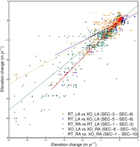
The two laser analyses yield R2 of 0.98 and 0.39 and slopes of the regression of 0.96 and 0.49, respectively. This indicates that both RT and XO measurements from ICESat are capable of resolving SEC trends within the drainage basin but that they are indeed affected by the more noisy SEC-5 signal. This dataset covers a larger region making it more exposed to spatial changes in the SEC trend, which are lost in the averaging of XO estimates. This naturally introduces an offset.
The analyses of RA vs. LA data show an offset in the resolved SEC signal. As nei-ther of the compared datasets are based on the same temporal or spatial resolution, firm conclusions cannot be drawn. It is, however, clear that the altimeters resolve the rate of thinning differently. The RT measurements – based on the highly accu-rate SEC-1 and -3 – agree well, which is positive considering the different types of altimeters as well as the geographical constraint to the quickly-changing drainage basin. Thus, RT analyses from RA provide comparable results with those from LA. The XO measurements show a poorer correlation, with SEC-8 resolving a greater variation in the SEC signal. This is partly due to the different altimeters and spa-tial resolutions, and partly to the lack of relocating the SEC-10 measurements, the latter thus demonstrating the necessity for doing so.
Hence, the above also explains the observed disagreement in the final analysis, namely that of RT and XO for RA data. The observations from SEC-1 proved highly accurate, and therefore the observed difference is believed to result from the methods used for obtaining the results – not the use of either RT or XO.
To summarize, the best SEC results for the given sensors and techniques arise from: LA: SEC-3’s RT solution and SEC-8’s XO method; RA: SEC-1’s RT solu-tion and SEC-9’s XO method. The latter is based on the lack of slope-correcting SEC-10, the smaller SEC-9 errors, and the corresponding better validation results. Therefore, it is believed that a lowering of the spatial resolution to better agree with the RA footprint will significantly improve the results. The respective datasets are discussed in further detail below.
Table 6. Results from the inter-comparison of a selection of the Round Robin results. The search radius used for finding overlapping grid cells is based on the spatial resolution given in Table 2, while “diff” holds the dH/dtdifference for the groups in question.
Participants Method Sensor Search # of Mean R2
Slope
radius points (diff)
(km) (m yr−1)
SEC-3–SEC-8 RT vs. XO Laser 1 226 -0.03 0.98 0.96
SEC-5–SEC-8 RT vs. XO Laser 1 493 -0.13 0.39 0.49
SEC-1–SEC-3 RT Radar vs. laser 5 3,935 -0.07 0.84 0.77
SEC-8–SEC-10 XO Radar vs. laser 10 76 0.08 0.53 0.46
[image:14.612.112.472.578.665.2]−6 −5 −4 −3 −2 −1 0 1 −6
−5 −4 −3 −2 −1 0 1
Elevation change (m yr−1)
Elevation change (m yr
−1
)
RT_LA vs XO_LA (SEC−3 − SEC−8) RT_LA vs XO_LA (SEC−5 − SEC−8) RT_RA vs RT_LA (SEC−1 − SEC−3) XO_LA vs XO_RA (SEC−8 − SEC−10) RT_RA vs. XO_RA (SEC−1 − SEC−10)
Figure 4. Scatter plots from inter-comparing a selection of the Round Robin results: cross-overs vs. repeat-track for radar and laser altimetry and radar vs. laser altimetry for both methods. The x-axis depicts the first-mentioned submission in the legend and the y-axis the latter. See Table 6 for the corresponding statistics.
5. Discussion
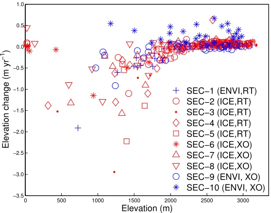
Figure 5 illustrates the relationship between the RR elevations and dH/dtvalues. A random subset has been plotted to optimize the visualization. Where elevations have not been supplied, they have been derived from the GIMP DEM. Generally agreeing, near-zero dH/dt values are found in the interior while disagreements occur further out towards the coastal margin. This pattern follows that of the error estimates, which increase with a lowering altitude. The observed changes in the interior are small, and both LA and RA perform well, regardless of the method. The largest offsets are found for SEC-10 due to the missing slope-correction. Closer to the coastal margin, a disagreement arises due to data errors, different data locations, and different routines applied for the SEC estimation. Most XO results are near-zero due to the data locations typically being on higher elevations, far from the glacier outlet, as well as averaging of the observations over larger grid cells. Collaborations with one of the XO participants demonstrated the effect of the latter: A simple experiment in which the results were downscaled to 1 km×1 km grid cells revealed a much better agreement with validation data and hence a significant improvement of the data accuracy. This further illustrated the advantage of applying a spatial resolution corresponding to the given footprint size (B. Gunter, pers. comm.).
[image:15.612.153.430.52.341.2]0 500 1000 1500 2000 2500 3000 −3.5
−3.0 −2.5 −2.0 −1.5 −1.0 −0.5 0.0 0.5 1.0
Elevation (m)
Elevation change (m yr
−1
)
[image:16.612.152.431.53.273.2]SEC−1 (ENVI,RT) SEC−2 (ICE,RT) SEC−3 (ICE,RT) SEC−4 (ICE,RT) SEC−5 (ICE,RT) SEC−6 (ICE,XO) SEC−7 (ICE,XO) SEC−8 (ICE,XO) SEC−9 (ENVI, XO) SEC−10 (ENVI, XO)
Figure 5. Subset of surface elevation vs. dH/dtvalues.
the few XO points, the RT analysis is investigated further. The focus lies on the coastal region, i.e. observations below 2000 m altitude. This yields 713 estima-tion points with a mean(diff) of −13 cm yr−1
, i.e. a larger difference than for the whole area, −7 cm yr−1
. For mass balance estimates, assuming only ice and an ice density of ρice = 917 kg m−3, this corresponds to an additional mass loss of
20 Gt yr−1
for the area, A, of 1.7×10⁵ km2. The change rate has been estimated
cf. dM/dt =ρice×(A×dH/dt), i.e. without accounting for SEC changes due to
firn compaction and surface mass balance variability as in Hurkmans et al. (2014). Considering a total GrIS mass loss of 263±30 Gt yr−1
for the period 2005–2010 (Shepherd et al. 2012), the SEC offset corresponds to a difference of 7%, i.e. a relatively small contribution. The above is a crude estimate for the specific ob-servation area and based on obob-servations with different spatial resolutions and observation periods. A more in-depth investigation of the RA-LA SEC differences is described by Sørensen et al. (2014), who compared 2003–2009 SEC trends de-rived from ICESat and Envisat data, respectively, and sampled to a similar spatial resolution. They found a correlation with changes in the accumulation rate and firn air content, and that the specific pattern is highly complex as it varies for different climatic zones and conditions. A full understanding of the changes there-fore requires in-depth analyses of accumulation, air content of the firn, surface temperature, melt, etc. This indicates that the offsets found in the RA vs. LA inter-comparisons only represent this specific region.
Part of the RA-LA SEC differences are due to backscatter of the RA echoes, an effect that varies throughout the ice sheet and is at a maximum in the interior (Legresy et al. 2005). Several studies have demonstrated that it has a large seasonal cycle and varies greatly with the length of the observation period, however that it makes out a small contribution to elevation change rates: Wingham et al. (1998) found an average SEC correction of 1.1 cm yr−1
with variations of approximately ±30 cm yr−1
for 1992–1996 ERS data over Antarctica; over Greenland, Zwally et al. (2005) found a mean and STD of 0.02±2.36 cm yr−1
from 1992–2002 ERS data, while Khvorostovsky (2012) found a mean correction of 0.35 cm yr−1
with variations exceeding ±3 cm yr−1
cor-rection therefore provides an important, however small, contribution to the final SEC estimates.
The fact that the adjustment does indeed affect the change detection has lead to a deeper investigation of the correction’s impact on the RA submissions and the po-tential conversion of these into estimates of mass balance changes; all participants accounted for backscatter, and one participant agreed to submitting additional re-sults for analyses covering both the given observation area and the entire GrIS. For the Jakobshavn Isbræ basin, the mean dH/dt signal changed by 1 cm yr−1
while variations ranged from −19 cm yr−1
to +11 cm yr−1
. For the ice sheet, the mean was 6 cm yr−1
with variations from −77 cm yr−1
to +39 cm yr−1
. Converting a 1 cm yr−1
backscatter correction into mass balance changes, and using a GrIS area of 2.166×10⁶ m2, yields mass losses of approximately 2 Gt yr−1
and 20 Gt yr−1
, respectively, for the two areas. The latter corresponds to a <10% adjustment of the GrIS volume rate and therefore makes out a relatively small improvement. This confirms that the adjustment for backscatter does make out a small contribu-tion to the SEC estimacontribu-tion and, therefore, the conversion hereof into mass balance changes.
An interesting observation in the ICESat datasets is that in spite of the par-ticipants using the same data release (R33) and some the same method, e.g. RT with LSq, the results differ. This is partly due to varying processing and estima-tion schemes, such as slightly different data rejecestima-tion criteria and LSq techniques, i.e. weighted, unweighted and multi-variate approaches, respectively. An additional reason is the inter-campaign biases, which vary with time thus affecting the accu-racy of the ICESat elevation measurements. Different groups have obtained dif-ferent bias estimates for the same dataset, and none of them have applied the Gaussian-Centroid part of the bias as discussed by Borsa et al. (2014). In spite of this, SEC-3’s results are found to be highly accurate and thus demonstrate an op-timal solution for change detection using LA. The group that provided these data solved for the surface slope and elevation changes using a multi-variate LSq tech-nique, and residual elevations from the regression exceeding 5 m were iteratively discarded to ensure each estimation value to be based on ≥ 10 footprints from at least four epochs covering a minimum of two years. Furthermore, the method rejected SEC estimates if the standard error exceeded 0.5 m yr−1
ensuring the inclusion of estimates with a high accuracy only.
Minimizing the errors is important. However, in order to ensure confidence in the final results it is equally important for the errors to reflect the nature of the observation area. This is possible when using the methods by SEC-5, -6, and -8: The estimates from SEC-5 and -8 are based on contributions from the dH/dttrend as well as the observations themselves, the data errors being included by adding a data covariance matrix into the least-squares fit. SEC-6’s errors are computed as the STD of the dH/dt values within any given grid cell, thereby providing more of a measure of the surface variability within each grid cell than an assessment of the accuracy of the technique. As such, an observed SEC variability translates into the error estimates, hence explaining the generally higher XO values particularly near the coastal margin. Thus, both methods yield larger errors mainly in highly dynamic and topographically rough areas, and this presumably makes the estimates more realistic.
Robin are the great potential in both RT and XO analyses, best visible for LA due to the higher data accuracy, and, most importantly, also clear for RA RT analyses: Investigations of SEC-1’s results demonstrate RA’s capabilities of resolving SEC throughout the GrIS, albeit with larger errors than in LA studies. Therefore, an iterative linear least-squares approach applied to RA RT data in which e.g. sur-face slope and backscatter parameters (leading edge width, trailing edge slope, and backscatter) are solved for is promising. The XO analyses show that LA accurately resolves the SEC signal, and that RA are capable of the same given relocation of the measurements and the spatial resolution corresponding to the altimeter foot-print. Therefore, SEC-9’s linear-sinusoidal fit with the application of a backscatter correction and for smaller grid cells are expected to provide the best RA XO results. Thus, a combination of RT and XO modules will allow for exploiting the re-spective high spatial coverage and high accuracy to precisely map SEC throughout the ice sheet, i.e. both in interior and margin regions. Based on the results from SEC-1, a spatial resolution of 5.0 km×5.0 km is a sufficient trade-off between the resolution achievable with RA and the final SEC accuracy. This shows great potential for the creation of an extensive SEC dataset based on RA from ERS, Envisat, CryoSat-2, and, in the longer term, Sentinel-3. Not only will it yield a time series based on more than two decades of observations; the greater amounts of observations overlapping in time and space will also help reducing estimation errors.
Due to different observation periods and flight times, completely agreeing ac-quisition times of the data used in the RR analysis cannot be achieved. This will introduce a difference between the RR and ATM validation dH/dttrends, which, if not accounted for, affects the comparison of the two types of data. The airborne campaigns are typically conducted in April/May or August, whereas ICESat data is only available in the periods of active lasers. Thus, when comparing a trend based on ATM data obtained in May with one derived from altimetry data ac-quired in e.g. October/November, the intermediate surface elevation changes must be accounted for. This elevation difference can, theoretically, be corrected for us-ing a Positive Degree Day model such as that by van den Broeke et al. (2010). It is based on the RACMO2/GR regional atmospheric climate model for Greenland (van Meijgaard et al. 2008) as well as observations from three Automatic Weather Stations located in Jakobshavn’s ablation zone. It calculates the degree day factors for snow and ice, respectively, i.e. a measure of the melt per positive degree-day. Given knowledge on what is melting, an estimate of the vertical surface change can be found. Problems with such a model are e.g. the sparsity of weather stations throughout the ice sheet, and the lack of observations of the exact composition of the surface material (e.g. ice, firn, or snow). Further complications arise as it does not account for precipitation, for which the rates are highest in the southern parts of the GrIS (Ettema et al. 2009; Sasgen et al. 2012). As the precipitation pat-tern changes in both time and space, the exact rates with which this happens are needed. They are, however, unknown. The lack of observations also distort mass balance approaches where a flux-balance and surface mass balance estimates can be used to infer the vertical surface change. Additional error sources are the poorly known density needed for such estimates as well as the seasonal variability of all of the above.
This indicates the difficulty in estimating an accurate vertical correction term to be applied to the ATM SEC trends. However, when applying the model and using a threshold temperature of T0 =−5◦C in order to include (nearly) all melt days
meters, i.e. less than the dynamical thinning observed in the area.
6. Conclusions
Several studies have been performed on the estimation of surface elevation changes (SEC) of the Greenland Ice Sheet using altimetry, e.g. Zwally et al. (2005, 2011); Sørensen et al. (2011); Khvorostovsky (2012). The most commonly applied methods are the repeat-track (RT) and cross-over (XO) techniques based on either laser or radar altimetry. In order to assess the quality of the respective SEC solutions, an inter-comparison exercise was conducted with contributions from the scientific community. Based on the findings, the best-performing SEC solution for ESA radar altimetry was identified. Ten datasets were received covering the Jakobshavn Isbræ drainage basin and derived using either radar (Envisat) or laser altimetry (ICESat). In order to evaluate the results, inter-comparisons of RT vs. XO studies and laser vs. radar data were performed. The submitted solutions were validated against SEC trends derived from temporally consistent and spatially collocated NASA ATM data. The conclusions can be summarized as follows:
• The spatial resolution of SEC estimates is higher with RT than with XO. Thus, RT allows for better resolving the surface changes along the coastal margin, such as along narrow ice streams.
• The XO method is advantageous as slope-induced errors from local topog-raphy can be ignored, however at the cost of a lower spatial data coverage. Validation shows a systematic bias, likely due to the spatial resolutions ex-ceeding the altimeter footprint size. Smoothing of the data thereby removes part of the SEC signal, particularly in margin regions. Therefore, using grid cells consistently sized relative to the footprint, the method is most suitable in the smooth interior ice sheet.
• In spite of the differences between the surface signals resolved from laser and radar altimetry, validation and inter-comparisons have revealed that radar data, particularly in RT analyses, can be used for accurately mapping SEC even in regions with high surface gradients.
For the ESA CCI SEC generation, we therefore propose a hybrid method in which RT and XO results are merged in order to maximise the spatial coverage and minimise the estimation errors. The merging will be carried out using geostatis-tical interpolation tools, i.e. the optimal gridding procedures known from collo-cation/simple kriging (Dermanis 1984; Goovaerts 1997; Hofmann-Wellenhof and Moritz 2005). The final SEC product will have a spatial resolution of 5 km×5 km, which is a good compromise between the resolution obtained with radar altimetry, the spatial data availability, and data errors. This is e.g. demonstrated by SEC-1 who used the same resolution to map elevation changes both in margin and interior regions. When to use either RT, XO, or combined results is based on a weighting of the error variances. The grid will predominately consist of RT results near repeat ground-tracks and along the coastal margin, the latter due to their higher spatial coverage, while XO estimates are found where ascending and descending ground-tracks intersect. Due to steep slopes along the margin, displacing measurement locations up-slope from nadir, XO locations are mostly confined to higher grounds. Results from this method are, however, used over as large a region as possible.
ESA web-site (http://products.esa-icesheets-cci.org/), and the 2002–2010 results are demonstrated by Sørensen et al. (2014). The implementation of ERS data has begun, and once a full understanding of the accuracy and performance of CryoSat’s InSAR altimeter has been reached, the inclusion of CryoSat-2 data will commence in order to bridge the gap between Envisat and Sentinel-3; launch of the latter is expected to take place in mid-2015 (ESA 2013b). The production of the final SEC grids is thereby underway.
Acknowledgements
We thank the European Space Agency Climate Change Initiative (ESA CCI) for supporting the analysis, and the Round Robin participants for taking the time to submit datasets and elaborate feedback sheets. We also thank B. Gunter for his extensive contribution to the analysis. The ICESat GLAS and ATM data were downloaded from NSIDC while Envisat data were available through ESA.
Author contributions:
J. F. Levinsen performed the analyses, wrote the paper, and produced the figures. K. Khvorostovsky unified the received datasets, participated in framing the analysis, and, along with F. Ticconi, A. Shepherd and R. Forsberg, assisted in data interpretation and the discussion of how to develop the SEC module. The remaining authors form the team of Round Robin participants and are listed in a random order based on the affiliation. All co-authors contributed to the discussions leading to the results presented in the paper.
Funding
The study was supported by the European Space Agency through the Ice Sheets CCI (grant number 4000104815/11/I-NB).
References
Arthern, R. J. 1997. ”The impact of climate variability on the determination of ice-sheet mass balance using satellite radar altimetry.” Ph.D. thesis, University of London, United Kingdom.
Ashcraft, I. V., and D. G. Long. 2005. ”Observation and Characterization of Radar Backscatter Over Greenland.” IEEE Transactions on Geoscience and Remote Sensing
43(2): 225–237, doi:10.1109/TGRS.2004.841484.
Bamber, J. L. 1994. ”Ice sheet altimeter processing scheme.” International Journal of
Remote Sensing 15: 925–938, doi:10.1080/01431169408954125.
Bamber, J. L., S. Ekholm, and W. B. Krabill. 2001. ”A new, high-resolution digital eleva-tion model of Greenland fully validated with airborne laser altimeter data”.Journal of Geophysical Research - Solid Earth106.
Borsa, A. A., G. Moholdt, H. A. Fricker, and K. M. Brunt. 2013. ”A range correction for ICESat and its potential impact on ice sheet mass balance studies”.The Cryosphere 8: 345–357, doi:10.5194/tcd-8-345-2014.
Brenner, A. C., R. A. Blndschadler, R. H. Thomas, and H. J. Zwally. 1983. ”Slope-induced errors in radar altimetry over continental ice sheets.” Journal of Geophysical Research
Brenner, A. C., J. P. DiMarzio, and H. J. Zwally. 2007. ”Precision and accuracy of satellite radar and laser altimeter data over the continental ice sheets.”IEEE Transactions on
Geoscience and Remote Sensing 45(2): 321–331, doi:10.1109/TGRS.2006.887172.
Davis, C. H. 1997. ”A Robust Threshold Retracking Algorithm for Measuring Ice-Sheet Surface Elevation Change from Satellite Radar Altimeters.”IEEE Transactions on Geo-science and Remote Sensing 35(4): 974–979, doi:10.1109/36.602540.
Dermanis, A. 1984. ”Kriging and collocation – a comparison.”Manuscripta Geodaetics 9: 159–167.
ESA. ”ESA Climate Change Initiative”. 2011a. http://www.esa-cci.org/.
ESA. ”ENVISAT ALTIMETRY Level 2 User Manual”. Version 1.4. Issued October 2011. 2011b. https://earth.esa.int/pub/ESA DOC/ENVISAT/RA2-MWR/PH light 1rev4 ESA.pdf.
ESA. ”Ice Sheets Essential Climate Variable”. 2013a. http://www.esa-icesheets-cci.org/. ESA. ”Sentinel 3”. 2013b.
https://earth.esa.int/web/guest/missions/esa-future-missions/sentinel-3.
Ettema, J., M. R. van den Broeke, E. van Meijgaard, W. J. van de Berg, J. L. Bamber, J. E. Box, and R. C. Bales. 2009. ”Higher surface mass balance of the Greenland ice sheet revealed by high-resolution climate modeling.” Geophysical Research Letters 36, doi:10.1029/2009GL038110.
Flament, T., and F. R´emy. 2012. ”Dynamic thinning of Antarctic glaciers from along-track repeat radar altimetry.” Journal of Glaciology 58(211): 830–840, doi:10.3189/2012JoG11J118.
Forsberg, R., Keller, K., and Jacobsen, S. M. 2002. ”Airborne lidar measurements for Cryosat validation.” In Geoscience and Remote Sensing Symposium, 2002. IGARSS ’02. 2002 IEEE International, Volume 3. 24–28 June 2002. 1756–1758.
Fu, L. L., and A. Cazenave. 2001. ”Satellite Altimetry and Earth Sciences: A Handbook of Techniques and Applications”. Academic Press.
Goovaerts, P. 1997. ”Geostatistics for Natural Resources Evaluation.” In Applied Geo-statistics Series, Oxford, UK: Oxford University Press, ISBN 0-19-511538-4.
Gray, L., Burgess, D., Copland, L., Cullen, R., Galin, N, Hawley, R., and Helm, V. 2013. ”Interferometric swath processing of Cryosat data for glacial ice topography.”
The Cryosphere 7(6): 1857–1867, doi:10.5194/tc-7-1857-2013.
Gunter, B. C., O. Didova, R. E. M. Riva, S. R. M. Ligtenberg, J. T. M. Lenaerts, M. A. King, M. R. van den Broeke, and T. Urban. 2013. ”Empirical estimation of present-day Antarctic glacial isostatic adjustment and ice mass change.”The Cryosphere
8(2): 743–760, doi:10.5194/tcd-8-743-2013.
Hawley, R. L., Shepherd, A., Cullen, R., Helm, V., and Wingham, D. J. 2009. ”Ice-sheet elevations from across-track processing of airborne interferometric radar altimetry.” Geo-physical Research Letters 36(22). doi:10.1029/2009GL040416.
Helm, V., Humbert, A., and Miller, H. 2014. ”Elevation and elevation change of Greenland and Antarctica derived from CryoSat-2.”The Cryosphere8: 1539–1559, doi:10.5194/tc-8-1539-2014.
Hofmann-Wellenhof, B. and H. Moritz. 2005.Physical Geodesy. 2nd edn. Wienna, Austria: Springer-Verlag.
Howat, I. M., I. Joughin, and T. Scambos. 2007. ”Rapid changes in the discharge from Greenland outlet glaciers.”Science 315: 1559–1561, doi:10.1126/science.1138478. Howat, I. M., A. Negrete, T. Scambos, and T. Haran. 2014. ”The Greenland Ice Mapping
Project (GIMP) land classification and surface elevation datasets.”The Cryosphere Dis-cussion 8: 1–26, doi:10.5194/tcd-8-1-2014.
Hurkmans, R. T. W. L., J. L. Bamber, and J. A. Griggs. 2012. ”Brief communication ’Importance of slope-induced error correction in volume change estimates from radar altimetry’.”The Cryosphere 6: 447–451, doi:10.5194/tc-6-447-2012.
variability from ice-sheet-wide velocity mapping.”Journal of Glaciology 59(197): 415– 430, doi:10.3189/002214310792447734.
Joughin, I., B. E. Smith, D. E. Shean, and D. Floricioiu. 2014. ”Brief Communication: Fur-ther summer speedup of Jakobshavn Isbr.”The Cryosphere8: 209–214, doi:10.5194/tc-8-209-2014.
Khvorostovsky, K. 2012. ”Merging and analysis of elevation time series over Greenland ice sheet from satellite radar altimetry.”IEEE Transactions on Geoscience and Remote
Sensing 50(1): 23–36, doi:10.1109/TGRS.2011.2160071.
Khvorostovsky, K. 2013. ”Analysis of the Greenland ice sheet elevation time series from satellite altimetry.” In European Geosciences Union Meeting, poster ID: EGU2013-10054, Vienna, 7–12 April 2013.
Krabill, W. B., W. Abdalati, E. Frederick, S. Manizade, C. Martin, J. Sonntag, R. Swift, R. Thomas, and J. Yungel. 2002. ”Aircraft laser altimetry measurement of elevation changes of the Greenland Ice Sheet: technique and accuracy assessment.” Journal of
Geodynamics 34(3–4): 357–376.
Legresy, B., F. Papa, F. R´emy, G. Vinay, M. van den Bosch, O. Z. Zanife. 2005. ”EN-VISAT radar altimeter measurements over continental surfaces and ice caps using the ICE-2 retracking algorithm.” Remote Sensing of the Environment 95: 150 – 163, doi:10.1016/j.rse.2004.11.018.
Levinsen, J. F., I. M. Howat, and C. C. Tscherning. 2013. ”Improving maps of ice-sheet surface elevation change using combined laser altimeter and stereoscopic elevation model data.”Journal of Glaciology 59(215): 524–532, doi:10.3189/2013JoG12J114.
Liu, L., J. Wahr, I. M. Howat, S. A. Khan, I. Joughin, and M. Furuya. 2012. ”Con-straining ice mass loss from Jakobshavn Isbræ (Greenland) using InSAR-measured crustal uplift.” Geophysical Journal International 188: 994–1006, doi:10.1111/j.1365-246X.2011.05317.x.
Moholdt, G., C. Nuth, J. O. Hagen, and J. Kohler. 2010. ”Recent elevation changes of Sval-bard glaciers derived from ICESat laser altimetry.”Remote Sensing of the Environment
114: 2756–2767, doi:10.1016/j.rse.2010.06.008.
NASA. ”Operation IceBridge – IceBridge Data Portal.” 2013a. http://nsidc.org/icebridge/portal/.
NASA. ”Laser Operational Periods.” 2013b. http://nsidc.org/data/icesat/laser op periods.html. Nghiem, S. V., Steffen, K., Neumann, G., and Huff, R. 2005. ”Mapping of ice layer extent
and snow accumulation in the percolation zone of the Greenland ice sheet.”Journal of Geophysical Research - Earth Surface, 110(F2), doi:10.1029/2004JF000234.
Nielsen, K., S. A. Khan, G. Spada, J. Wahr, M. Bevis, L. Liu, and T. van Dam, T. 2013. ”Vertical and horizontal surface displacements near Jakobshavn Isbræ driven by melt-induced and dynamic ice loss.”Journal of Geophysical Research - Solid Earth118: 1837–1844, doi:10.1002/jgrb.50145.
R´emy, F., T. Flament, F. Blarel, and J. Benveniste. 2012. ”Radar altimetry measurements over antarctic ice sheet: A focus on antenna polarization and change in backscatter problems.”Advances in Space Research 50(8): 998–1006, doi:10.1016/j.asr.2012.04.003. Ridley, J. K. and K. C. Partington. 1988. ”A model of satellite radar altime-ter return from ice sheets.” International Journal of Remote Sensing 9: 601–624, doi:10.1080/01431168808954881.
Sasgen, I., M. van den Broeke, J. L. Bamber, E. Rignot, L. S. Sørensen, B. Wouters, Z. Martinec, I. Velicogna, and S. B. Simonsen. 2012. ”Timing and origin of recent regional ice-mass loss in Greenland.” Earth and Planetary Science Letters 333–334: 293–303, doi:10.1016/j.epsl.2012.03.033.
Scharrer, K., J. F. Levinsen, and F. Ticconi. 2013. ”Product Validation and Algorithm Selection Report for the Ice Sheets cci project of ESA’s Climate Change Initiative.” 2013. http://www.esa-icesheets-cci.org/.
Schutz, B. E., Zwally, H. J., Shuman, C. A., Hancock, D. and DiMarzio, J. P. 2005. ”Overview of the ICESat Mission.” Geophysical Research Letters 32, 21: 1944–8007, doi:10.1029/2005GL024009.
K. H. Briggs, D. H. Bromwich, R. Forsberg, N. Galin, et al. 2012. ”A Reconciled Esti-mate of Ice-Sheet Mass Balance.”Science 338: 1183–1189, doi:10.1126/science.1228102. Slobbe, D., R. Lindenbergh, and P. Ditmar. 2008. ”Estimation of volume change rates of Greenland’s ice sheet from ICESat data using overlapping footprints.”Remote Sensing of the Environment 112: 4204–4213, doi:10.1016/j.rse.2008.07.004.
Sørensen, L. S., S. B. Simonsen, K. Nielsen, P. Lucas-Picher, G. Spada, G. Adalgeirsdottir, R. Forsberg, and C. S. Hvidberg. 2011. ”Mass balance of the Greenland ice sheet (2003– 2008) from ICESat data – the impact of interpolation, sampling and firn density.”The Cryosphere5: 173–186, doi:10.5194/tc-5-173-2011.
Sørensen, L. S., S. B. Simonsen, R. Meister, T. Flament, R. Forsberg, J. F. Levinsen. 2014. ”Envisat derived elevation changes of the Greenland ice sheet, and a comparison to ICESat results in the accumulation area.” Remote Sensing of the Environment. In review.
van den Broeke, M., C. Bus, J. Ettema, and P. Smeets. 2010. ”Temperature thresholds for degree-day modelling of Greenland ice sheet melt rates.” Geophysical Research Letters
37, doi:10.1029/2010GL044123.
van Meijgaard, E., L. H. van Ulft, W. J. van de Berg, F. C. Bosveld, B. J. J. M. van den Hurk, G. Lenderink, and A. P. Siebesma. ”The KNMI regional atmospheric climate model.” Version 2.1, Tech. Rep. 302, R. Neth. Meteorol. Inst. De Bilt, the Netherlands. 2008. http://a.knmi2.nl/bibliotheek/knmipubTR/TR302.pdf.
Zwally, H. J., M. B. Giovinetto, J. Li, H. G. Cornejo, M. A. Beckley, A. C. Brenner, J. L. Saba, and D. Yi. 2005. ”Mass changes of the Greenland and Antarctic ice sheets and shelves and contributions to sea-level rise: 1992–2002.” Journal of Glaciology 51: 509–527, doi:10.3189/172756505781829007.
Zwally, H. J., J. Li, A. C. Brenner, M. A. Beckley, H. G. Cornejo, J. Dimarzio, M. B. Giovinetto, T. A. Neumann, J. Robbins, J. L. Saba, D. Yi, and W. Wang. 2011. ”Greenland ice sheet mass balance: distribution of increased mass loss with climate warming; 200307 versus 19922002.” Journal of Glaciology 57: 88–102, doi:10.3189/002214311795306682.