An extended two-dimensional borehole heat exchanger model for simulation of short and medium timescale thermal response

This is a repository copy of

An extended two-dimensional borehole heat exchanger model

for simulation of short and medium timescale thermal response

.

White Rose Research Online URL for this paper:

http://eprints.whiterose.ac.uk/89679/

Version: Accepted Version

Article:

Rees, SJ (2015) An extended two-dimensional borehole heat exchanger model for

simulation of short and medium timescale thermal response. Renewable Energy, 83. 518 -

526. ISSN 0960-1481

https://doi.org/10.1016/j.renene.2015.05.004

© 2015, Elsevier. Licensed under the Creative Commons

Attribution-NonCommercial-NoDerivatives 4.0 International

http://creativecommons.org/licenses/by-nc-nd/4.0/

eprints@whiterose.ac.uk https://eprints.whiterose.ac.uk/

Reuse

Unless indicated otherwise, fulltext items are protected by copyright with all rights reserved. The copyright exception in section 29 of the Copyright, Designs and Patents Act 1988 allows the making of a single copy solely for the purpose of non-commercial research or private study within the limits of fair dealing. The publisher or other rights-holder may allow further reproduction and re-use of this version - refer to the White Rose Research Online record for this item. Where records identify the publisher as the copyright holder, users can verify any specific terms of use on the publisher’s website.

Takedown

If you consider content in White Rose Research Online to be in breach of UK law, please notify us by

An extended two-dimensional borehole heat exchanger model for simulation of short

and medium timescale thermal response

Simon J. Reesa,⇤

a_{IESD, School of Engineering and Sustainable Development, De Montfort University, The Gateway, Leicester, LE1 9BH, UK.}

Abstract

Common approaches to the simulation of Borehole Heat Exchangers (BHEs) assume heat transfer in circulating fluid and grout to be in a quasi-steady state and ignore fluctuations in fluid temperature due to transport of the fluid around the U-tube loop. Such effects have been shown to have an impact on peak temperatures and hence operation of heat pumps systems when short time scales are considered. A model has been developed that combines a two-dimensional numerical model and models of the pipe loop components. A novel heat exchanger analogy is employed to calculate the heat exchanger outlet temperatures such that iterative procedures can be avoided and numerical stability is unconditional. These approaches result in a model that is computationally efficient and captures much of the short timescale dynamic effects represented in fully three-dimensional models. This is demonstrated by comparison with experimental data and by comparing two and three-dimensional model behaviour in the frequency domain. Predicted monthly outlet temperatures and heat transfer rates are furthermore shown to be in close agreement with experimental values and in good agreement with existing borehole heat exchanger models. The model is computationally efficient enough to allow use in routine analysis and design tasks.

Keywords: Borehole Heat Exchanger, Geothermal, Ground Source Heat Pump, Numerical Model

1. Introduction

The commonest form of ground heat exchanger used in ground-source heat pump applications are vertical borehole heat exchangers (BHE) consisting of heat exchanger pipes in U-tube form inserted into a drilled borehole and sealed with grout or other backfill material. Boreholes are typically 100-150 mm in diameter and drilled to depths of 100-300 m (Fig. 1). For all but the smallest capacity systems the BHE are installed in arrays spaced typically 5-15 m apart and ar-ranged in parallel circuits. The primary physical phenomena of interest in the study of heat exchanger performance are the dynamic conduction in the pipe, grout and surrounding soil/rock as well as convection at the pipe wall.

A number of models of BHE devices and system have been reported that may be used for heat exchanger design and sys-tem simulation tasks as well as analysis of Thermal Response Test (TRT) data. Models of BHE chiefly differ according to whether:

• two or three dimensions are considered;

• single or multiple boreholes can be represented;

• heterogeneous thermal properties are assumed;

• the representation of pipe and grout, and;

⇤_{Corresponding author. Tel.:+44 (0)116 257 7974}

Email address:sjrees@dmu.ac.uk(Simon J. Rees)

• treatment of circulating fluid transport.

Models can also be classified according to whether they adopt analytical[1, 2, 3], numerical or hybrid[4, 5, 6] ap-proaches. The question of dimensionality and to what level of detail the grout, pipe and fluid components are represented is related to both the time and length scales that are consid-ered.

Three-dimensional numerical conjugate heat transfer mod-els that discretize both the solid domains and the heat trans-fer fluid (as applied in a recent study of energy piles[7]) can arguably capture all these effects. Some models come close to this level of detail[8, 9, 10, 11]but stop short of fully dis-cretising the heat transfer fluid. Generally three-dimensional models remain computationally demanding and so are not commonly used for routine design and analysis tasks. Mod-els that are two-dimensional, analytical or hybrid in nature are more efficient but have some levels of approximation that need to be accepted.

Figure 1: A single U-tube Borehole Heat Exchanger.

a reference three-dimensional model [12]. We furthermore evaluate the short timescale response against that of the ref-erence model by making comparisons in the frequency do-main.

2. Background

We firstly consider the physical phenomena that are par-ticularly relevant to modelling behaviour at short time scales and then different approaches to modelling such character-istics.

2.1. Physical phenomena of interest

Over much of the length of a borehole heat exchanger the heat transfer driven by the heat fluxes at the pipe walls is predominantly in the radial direction. This implies that the temperature gradients are greatest near the pipes within the borehole. As the two ‘legs’ of the U tube are separated and generally have, at a given depth, different fluid temperatures there are significant local temperature gradients in the grout and so called ’short circuit’ heat fluxes between the adjacent pipes. If one is only considering medium and long timescales (e.g. the system design models using response factors and temporal superposition such as that of Hellström[13]) then these short timescale and localized dynamic effects can be ignored and it is reasonable to represent everything within the borehole by a system of thermal resistances. If one is in-terested in simulating system operation to evaluate heating and cooling system behaviour then it becomes necessary to simulate with short time steps and to consider physical phe-nomena that are more significant at short timescales. The short timescale effects that are apparent are:

• Temperature gradients within the borehole and ther-mal capacity of the grout;

• The thermal capacity of the heat transfer fluid;

• The dynamic transport of heat by the fluid moving around the pipe loop.

The combination of these physical phenomena tend to re-sult in both damping and delaying of the response of the heat exchanger to changes in inlet temperature. It has been shown to be particularly important to consider these effects if peak temperatures and interaction between the heat pump control system and the ground heat exchange system are to be con-sidered, for example, in residential systems where control is achieved by on-off cycling of the heat pump[14]. The large non-residential system analysed by Naicker showed the short timescale cyclic operation of the system to have a significant impact on overall system performance[15]. The ground heat exchanger system in this case had significant fluid content in the BHE (56 100m boreholes) but also the large diame-ter horizontal pipe system and was shown to have a highly damped response.

The physical process that has a further effect on the short timescale response is the dynamic transport of the circulating fluid and thermal diffusion along the pipes. The simple delay in inlet temperature changes being propagated through the U-tube could be expected to be important at short timescales if one considers that the nominal transit time of the fluid trav-elling through the U-tube could be of the order of a few min-utes with typical BHE depths and pipe velocities. In addition to a time delay, variations in inlet temperature are also dif-fused because fluid does not circulate in a ‘plug’ with uniform velocity but fluid at the centre of the pipe travels at higher velocity than the fluid near the pipe wall. Hence, fluid at the outlet will generally have been mixed with fluid in the pipe that entered the heat exchanger at an earlier time and probably at a different temperature. This is illustrated in Fig. 2. The longitudinal diffusion is theoretically maximized in laminar flow conditions and is generally Reynolds Number (Re) dependent. As Reynolds Numbers in BHE can be low— particularly in variable flow systems—these effects can be ex-pected to be noticeable. Both the thermal mass of the fluid and the diffusive transport process mean that swings in inlet temperature tend to be damped[14, 16].

L

τ = 0

T

˙

V

ˆ

v

¯

v

τ

= 1

Figure 2: Pipe fluid flow and longitudinal diffusion processes. A temperature pulse entering the pipe is transformed into a diffused response at the end of the pipe. The shape of the response at the outlet depends on the velocity profile and hence turbulence.

without heat transfer and variations in component concen-tration) but usually in the absence of high thermal mass sur-roundings[17, 18]. The problem has also been analysed in terms of the ‘delayed hot water problem’[19, 20, 21, 22]— the research question being how long does it take hot wa-ter to be delivered when the tap (faucet) on a cold pipe is opened? In these cases the pipe is modelled with thermal mass and this has the effect of further delaying the arrival of any hot water front.

2.2. Modelling short time scale behaviour

One approach to resolving the temperature gradients with the grout domain and taking account of its thermal capacity is to construct a two-dimensional numerical model in a plane perpendicular to the borehole axis (i.e. horizontal) with a sufficiently fine mesh. This was the approach taken by Yavuz-turk[23]who used an orthogonal grid and a pie-sector ap-proximation to the pipe geometry but did not explicitly rep-resent the fluid. This model was used to derive short term responses to step heat pulses and this data combined with g-function data to form a hybrid model suitable for both short and long timescale simulation[5]. Young[24]sought to ad-dress the exclusion of the fluid by applying a ‘buried cable’ analogy to include the effect of the fluid’s thermal capacity. These models do not take account of the dynamics arising from the transport of heat by the fluid, however.

Another approach to improving the representation of the thermal capacity of the grout is to use a lumped capacity ap-proach and associate discrete thermal mass (capacitances in an electrical analogy) with resistances in a network involv-ing the pipes, grout and borehole wall. Although this does not allow some of the steep temperature gradients inside the borehole to be resolved, it is computationally efficient and can be repeated in the axial direction to achieve a quasi-three dimensional representation of a single BHE. In this approach nodes can be included to represent a fraction of the pipe fluid volume at each level and these can be connected to represent fluid flow around the U-tube.

This approach is taken in Wetter and Huber’s EWS model

[25]using only a single capacitance to represent the grout. Oppelt et al. [26]have sought to address this limitation of the EWS model by dividing the grout into sectors so that each vertical layer of a double U-tube was represented by five lumped thermal capacitances. De Carli et al. [27] devel-oped a so-called Capacity Resistance Model (CaRM) and dis-cretized the borehole — including the circulating fluid — into several slices along its depth with each slice also discretized in the radial direction. Bauer et al. [28]used a simplified rep-resentation of the borehole components in the form of a net-work of resistances and capacitances in the TRCM model and discretized the borehole in the vertical direction in a similar way to the EWS and CaRM models. Fluid responses and ver-tical temperature gradients calculated over short timescales using this model compared favourably with those from a fully discretized finite element model.

3. Model development

The approach taken in the current work is to combine a two-dimensional numerical model constructed in the hor-izontal plane along with a discretized model of fluid flow around the pipe loop. This is intended to allow accurate rep-resentation of the dynamic heat transfer inside the borehole— given a reasonably fine numerical mesh—along with a rep-resentation of both the thermal capacity of the fluid and the effect of delayed transport of heat around the pipe loop. This is a simplification of an earlier three-dimensional model[12, 29] in which the circulating fluid was integrated with the borehole geometry. A simplified approach has been sought in the interests of computational efficiency. The model is im-proved over related two-dimensional models reported ear-lier[30, 31] in the way outlet temperature are calculated such that the model is more robust and its computational efficiency further improved. The two-dimensional models discussed above were (with the exception of Yavuzturks ’pie sector’ approach [23]) oriented in the axial-radial sense so that flow around the pipes was explicitly discretized but mod-elling of heat transfer inside the borehole limited to lumped capacitances and resistances. The advantage of applying a boundary-fitted (i.e. geometrically accurate) numerical model in a horizontal plane as proposed here, is that temperature gradients around the pipes are captured in some detail. Hence there thermal capacity of the grout and heat fluxes between the pipes can be well resolved as well as the borehole resis-tance (Rb) calculated accurately.

The two-dimensional numerical model component of the BHE model is derived from a Finite Volume Method solver that has previously been used in a fully three-dimensional model of a BHE[29]. The code applied in the latter model has been validated against reference analytical results for borehole resistance[32]such that resistance values can be re-produced with errors less than 0.1%[24, 12]. In this applica-tion a two-dimensional mesh of a borehole (i.e. using a mesh one cell deep) is used and the fluid is treated in a pipe model component described later. Convection/advection terms of the heat transfer equations accordingly do not need to be solved as they were in the three-dimensional model.

3.1. The numerical method

The Finite Volume Method has been used to discretize the integral form of the Fourier equation. The approach to dealing with non-orthogonal cell geometries has been to dis-cretize the equation in physical space using an approach sim-ilar to that described by Ferziger and Peri´c [33]. The pri-mary variables are defined at the hexahedral cell centroids on a block-structured mesh. The integral form of the Fourier equation solved here (leaving aside source terms) is:

@ @t

Z

V

⇢C TdV= Z

S

kr ·_{nTdS (1)}

with conduction heat transfer. The diffusion flux term in dis-crete form (FD

i ) is approximated by the sum of the fluxes

through each cell face. such that,

Z

S

kr ·_nTdS⇡X

i

F_iD (2)

where,iis the index for each face of the hexahedral cell. As-suming that the value of the temperature,T, over a particular face is well represented by the value at the face centroid, the diffusion heat flux can be approximated as:

F_iD= (kr_T·_n)_iSi (3)

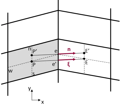
This requires a discrete method for finding the gradient of the temperature (r_T) at each cell face using the cell centroid values. A typical non-orthogonal cell, with local coordinates at the east cell face, is illustrated in Fig. 3. The coordinaten is defined in the direction normal to the face at its centroids, and the coordinate ⇠is defined on the line between neigh-bouring centroids which passes through the face at point e. In order to calculate the gradient of the variable at the cell face, the values of the variable at the cell centroids are used as they are the primary variables. The gradient is calculated using the valuesTPandTEat neighbouring centroids and the

distance between these points, LP,E(in Fig. 3 at the east face F_eD⇡_keSe(@T/@ ⇠)_e0) but this is only second-order accurate

if the grid is orthogonal. In order to preserve second-order accuracy the calculation of the gradient along the normal to the face at the centroid needs to be made using the values at pointsP0

andE0

. However, the values of the temperature at these points are not calculated explicitly and have to be interpolated from the cell centroid values. Consequently a deferred correction approach is used to calculating the flux as follows,

P E

n

s w

e

P’ n E’

ξ

x y

e'

Figure 3: A typical non-orthogonal finite volume cell highlighting the fluxes at the east face and the respective cell centroids.

FD e =keSe

Å_@T

@ ⇠

ã

e0

+k_eS_e

ïÅ_@T

@n ã

e

−

Å_@T

@ ⇠

ã

e0

òol d

(4)

During the iterative solution process, the terms in the square brackets are calculated from the previous estimates of the variables. When the solution is converged the first and the third terms cancel each other to leave the term that only uses the gradient along the face normal. Central differencing is used to estimate the gradients such that,

Å_@T

@ ⇠

ã

e0

= TE−TP

LP,E

and

Å_@T

@n ã

e

= TE0−TP0

LP0_,E0

(5)

Values at the locations P0 and E0

are interpolated from the cell centroid values using the gradient of the variable at that point which, in turn, can be calculated from the face centroid values by applying Gauss theorem[33]. Temporal discretization can be first or second order backwards implicit using a method that allows for variable time steps[34]. The sets of algebraic equations arising from the discretization on the multi-block mesh are solved using an iterative method based on the Strongly Implicit Procedure[35]adapted to al-low communication of data across block boundaries during the iterative procedure and has been found to be very robust. The borehole heat exchanger geometry has been discretized using a three-dimensional multi-block boundary fitted struc-tured mesh and this has been defined using an in-house util-ity[36]that uses a two-dimensional definition of the bore-hole components and extrudes this to form a 3D mesh such as that shown in Fig. 4. Individual blocks define the pipes and two blocks are used to define the grout material within the borehole. Multiple blocks may be used to define the sur-rounding ground depending on the far field boundary shape and also–by repeating similar borehole block arrangements– adjacent boreholes.

Figure 4: A multi-block representation of a borehole heat exchanger mesh (symmetry assumed at the bottom edge). Colours indicate the extent of each block. Only the central region of the mesh surrounding the borehole is shown.

3.2. Generic boundary conditions

All boundary conditions in the numerical model are im-plemented as variations of a generic form. This generic form is defined by three coefficients (A,B,C) multiplying the vari-able (T), the gradient of the variable normal to the boundary and a constant term respectively as indicated in Eq. (6).

A T+Bd T

The coefficients are defined for each boundary condition instance. This generic form allows Dirichlet, Neumann and mixed boundary condition types to be defined. Where the temperature is the primary variable the common forms of these boundary conditions correspond to fixed temperature, fixed flux (including the adiabatic condition) and convective heat transfer conditions. The corresponding values of the coefficients are indicated in Table 1. The generic boundary condition has been adapted to allow the boundary conditions inside the borehole to be applied directly, as will be shown in the following section.

3.3. Pipe surface boundary conditions

In two-dimensional models of borehole heat transfer it is necessary to define the relationship between the temper-ature at the pipe boundary surface (or borehole wall) and both the fluid inlet and outlet temperatures. For example, a mean borehole fluid temperature can be defined which is the arithmetic mean of the inlet and outlet temperatures and this temperature applied in a convective boundary condition. However, as the outlet temperature is unknown it is neces-sary to guess the initial mean borehole temperature, calcu-late the flux using the numerical model and then update the outlet temperature from the overall fluid heat balance. In order to make the borehole and outlet temperatures consis-tent it is necessary to iterate and this is both computationally inefficient and is not guaranteed to converge (particularly with small time steps). Results are furthermore not guaran-teed to comply with the second law of thermodynamics i.e. borehole temperature being bounded by the inlet and outlet temperatures. Other assumptions about pipe or fluid tem-peratures can be made but generally require similar iterative procedures to find an outlet temperature consistent with flux calculated by the numerical model.

The proposed approach avoids this iterative process by as-suming the pipe surface temperature does not vary along its length (which is consistent with a two-dimensional represen-tation) and makes an analogy with an evaporating-condensing heat exchanger. This approach is similar to that applied in the modelling of embedded pipes in underfloor heating sys-tems by Strand[37]. The heat exchanger can be character-ized by an effectiveness parameter,"which is the proportion of heat transferred compared with the maximum theoretical heat transfer. A numerical model boundary condition of the form defined in Eq. (6) can be developed as follows.

The overall heat balance can be defined by the maximum possible temperature difference (that between the inlet and the pipe surface) and the effectiveness as follows,

Qp="mC˙ '

Tin−Tp (

(7)

For a heat exchanger with constant surface temperature along its length the effectiveness is given by,

"=1−_e−N T U ₍₈₎

and this is related to the total pipe area (S = 2⇡rpL) and

fluid heat transfer coefficient by the Number of Transfer Units

(NTU) according to,

N T U= 2⇡rpLhp

˙

mC (9)

The pipe convection coefficient,hpis modelled using the well

known Dittus-Boelter equation such that,

hp=

0.023Re4/5P rnkf

2⇡r_p (10)

where the exponent,n, is 0.4 or 0.3 according to heat transfer being by heating or cooling.

The fluid heat balance defined by Eq.(7) in this two-dimensional representation is equivalent to the instantaneous flux at the pipe wall. The pipe wall is the boundary of the numeral model domain and at this surface the fluid convective flux is balanced with the conduction heat flux. The overall fluid heat balance is therefore equivalent to the total conduction flux at this boundary so that,

"mC˙ 'Tin−Tp (

=−_kSd T

d n (11)

This equation can be rearranged to show a form similar to the numerical model boundary condition defined in Eq.(6) such that,

"mC˙

S T−k

d T d n−

"mC˙

S Tin=0 (12)

The boundary condition coefficients are consequently: A= ("mC˙ )/S; B = −_{k; C} = Tin("mC˙ )/S. This is also noted

in Table 1. This heat exchanger boundary condition can be applied given only the inlet temperature and flow rate. So-lution of the finite volume equations gives the pipe heat flux directly and subsequently the overall borehole heat transfer rate and hence outlet temperature. No iteration is required and, as the numerical method is implemented in fully implicit form (i.e. backwards differencing in time) it is uncondition-ally stable. The model is therefore more efficient than other approaches[23, 30, 31]and is useful over a wide range of time step sizes.

3.4. Modelling of fluid response

The approach taken here to modelling the short-timescale dynamic effects related to the circulation of heat transfer fluid in the BHE circuit, is to add a discretized model of flow through a pipe that incorporates the effects of longitudinal dispersion and thermal capacity. This concept was investigated by He

[29]but is implemented here with a more sophisticated pipe model and a different approach to modelling heat transfer from the pipe and coupling with the numerical element of the model.

Boundary condition type Form A B C

Fixed Temperature (Dirichlet) T=T_b −_{1.0 0.0 T}

b

Fixed Flux (Neumann) q_b=−_kd T

d n 0.0 k qb

Convection (Mixed) −_kd T

d n =hc(Te−T) hc −k hcTb

Heat exchanger "mC˙ 'Tin−Tp (

=−_kSd T

d n ("mC˙ )/S −k Tin("mC˙ )/S

Table 1: Thermal boundary condition types and their relationships to the generic boundary condition form.

convection-diffusion model of the following partial differen-tial form,

@T(x,t)

@t +v

@T(x,t)

@x +D

@2_T(x,t)

@x2 =0 (13)

In this Axial Dispersion Plug Flow (ADPF) model the diffusion coefficient, D, is an effective value that depends on velocity profile and therefore Reynolds number, and was empirically determined in early work [38]. A commonly used approxi-mation to this model is to represent the pipe by a series of well stirred tanks, often referred to as the N-continuously stirred-tanks (N-CST) model. This model has been used in thermal systems applications[40]and BHE models[29]with some success but, although it is computationally efficient, tends to be overly diffusive. This model is somewhat sensitive to the number of tanks, NC S T, chosen to represent the pipe. Wen

and Fan[17]derived an expression to find the appropriate number of tank cells according to Peclet Number (Pe) that gave a good approximation to ADPF behaviour:

N_{C S T} = v L

2D= Pe

2 (14)

Another form of simplified model is formulated by combin-ing a plug-flow model (i.e. simple time delay) with continu-ously stirred tanks: the PFNCST model[41]. This model has recently been implemented and evaluated by Skoglund and Dejmek[42]and shown to be accurate when compared to an-alytical solutions to the ADPF equation but also less sensitive to the choice of the number of continuously stirred tanks in clouded in the model (only 16 tanks were required to achieve close agreement). This is the form of pipe model adopted in the current work. The model and its integration with the nu-merical model is shown schematically in Fig. 5. The model is defined by heat balances on each tank element and the time delay associated with the inlet plug-flow element as follows,

T_i=0(t) =Tin(t−⌧0) (15)

⇢C VN

@Ti

@t +⇢CV˙(Ti−Ti−1) =0 (16)

In this model the fluid transit time (⌧) is divided between that associated with the initial plug-flow element (⌧₀) and the remaining time in transit through the stirred tank elements. To retain the required total transit time it is required that

N⌧_N=⌧−_⌧

0. Skoglund and Dejmek[42]showed that the

model agrees with the ADPF representation when,

⌧_N= v

t2L D

N v3 =⌧ v

t 2

N Pe (17)

These equations consequently allow the size of the plug-flow Length/Volume to be determined for a given number of tanks. The other model coefficient in the model is that of the effec-tive diffusion coefficient,Dand we choose this according to Reynolds Number according to the recommendation of Wen and Fan[17]as follows,

D L v =

2rp

L (3.0⇥10 7_Re−_2.1

+1.35Re−0.125) (18)

4. Model validation

Model validation has been attempted by making compar-isons with experimental borehole heat exchanger data over both short and long timescales. We have also made compar-isons between the extended two-dimensional model and the fully three-dimensional model that shares the same numeri-cal method and which we regard as a reference model[12]. Experimental data is that collected at Oklahoma State Uni-versity reported by Hern[43]and Gentry[44]and used in other inter-model comparisons[45]. The borehole dimen-sions and properties are shown in Table 2. The ground ther-mal conductivity value was taken as the mean of three values determined by Thermal Response Tests.

4.1. Short time-scale response

plug ßow element N ideal stirred tank elements

˙

V, ¯v,Tin Tout

h=εmC_S˙

1 h=

εmC˙

S2

V0, τ0 VN, τN=VN/V˙

2D numerical model

Tbottom

Tp,1 Tp,2

Figure 5: The extended 2D numerical model showing coupling of the numerical boundary and pipe components.

Parameter Value Units

Borehole depth 74.68 m

Undisturbed ground temperature 17.3 °C

Fluid flow rate 0.212 L/s

Borehole diameter 114.3 mm

Pipe inner diameter 21.82 mm

Pipe outer diameter 26.67 mm

Borehole shank spacing 20.32 mm

Pipe thermal conductivity 0.3895 W/(m.K) Pipe thermal capacity 1770 kJ/(m3_.K)

Grout thermal conductivity 0.744 W/(m.K) Grout thermal capacity 3900 kJ/(m3_.K)

Ground thermal conductivity 2.550 W/m.K Ground thermal capacity 2012 kJ/(m3_.K)

Fluid thermal conductivity 0.598 W/(m.K) Fluid thermal capacity 4184 kJ/(kg.K)

Table 2: Experimental BHE dimensions and thermal properties[45].

much of the fluctuations are damped out by the exchange of heat to-and-from the pipe and grout within the borehole and there is little interaction with the ground outside the bore-hole. Responses are not only delayed (out of phase) by more than the nominal fluid transit time but are strongly damped in these cases[29].

Predicted responses to sinusoidal variations in inlet tem-perature are shown in the frequency domain in Fig.s 6 and 7 for the proposed extended model and the reference three-dimensional model. Fig. 6 shows the variation in ampli-tude of the predicted outlet temperature over a range of ex-citation periods between one minute and one hour and Fig. 7 shows the predicted delay. The predicted output of the two-dimensional numerical model without the coupled pipe model is also shown and indicates how two-dimensional mod-els that ignore short time-scale effects, perform very differ-ently to a fully three-dimensional model that represents the fluid circulation explicitly. The trends in both amplitude

re-duction and delay show good agreement between the ref-erence model and the proposed extended model. The two-dimensional numerical model without the pipe extension shows little damping of higher frequency variations in inlet temper-ature (only that related to the dynamic effects of grout ther-mal capacity) and virtually no time delay.

4.2. Dynamic characteristics

0 0.1 0.2 0.3 0.4 0.5 0.6 0.7

0.0002 0.002 0.02

A

m

pl

it

ude

ra

ti

o

Frequency (Hz)

3D model 2D model

extended 2D model

Figure 6: Outlet temperature Amplitude ratio calculated over a range of sinusoidal input temperature excitation frequencies. Comparison is made with the 3D reference model results[29]

0 1 2 3 4 5 6

0.0002 0.002 0.02

P

ha

se

l

ag (c

yc

le

s)

Frequency (Hz) 3D model

2D model extended 2D model

Figure 7: Outlet temperature lag calculated over a range of sinusoidal in-put temperature excitation frequencies .Comparison is made with the 3D reference model results[29]

the experiment have been used as boundary conditions to the extended model and predicted values of outlet temperature compared with recorded values. During the experiments the heat pump was switched on and off intermittently and the circulating pump ran continuously. Data showing a cycle of operation in the 15th day of operation (March 15, 2005) are shown in Fig. 8. When the heat pump switches on the inlet temperature falls quickly by approximately 3K. The experi-mental results show that there is no response observable at the outlet until more than four minutes later. Later in the operating cycle the outlet temperature falls at a similar rate to that of the inlet. At the end of the operating cycle the inlet temperature shows a sharp increase and a similar delay in the outlet temperature response can be observed. The delay in the response is of the same magnitude as the nominal transit time of the U-tube which, at the flow rate in question, is 4.4 minutes.

9 10 11 12 13 14 15 16

15 15.25 15.5 15.75 16 16.25 16.5

F

lui

d t

em

pe

ra

ture

(

!

C)

Hour

inlet outlet 2D model 3D model extended 2D model

Figure 8: Minutely outlet temperatures compared for data collected on March 15[43].

The outlet temperature predicted by the extended two-dimensional model can be seen to demonstrate very similar delays in response at both the beginning and the end of heat pump operation. This response is also similar to that shown by the reference three-dimensional model[29]. During the operating period the outlet temperature prediction follows the experimental data closely. The significance of modelling the fluid circulation has been highlighted by including data in Fig. 8 from the two-dimensional model that does not in-clude the pipe element. The outlet temperature in this (and probably other) 2D models necessarily responds instantly to changes in inlet temperature.

4.3. Ground heat transfer

The validity of the heat exchanger analogy used to de-fine heat transfer at the pipe in the proposed model has been investigated by examining predictions of ground heat trans-fer over 16 months of the available experimental data. Inlet temperature and flow rate data at hourly intervals has been used as the mode boundary conditions in these tests in much the same way as the inter-model comparison reported earlier

[45]. Predicted monthly net heat transfer and mean outlet temperatures are compared in Figs. 9 and 10 respectively. The model data are shown compared with the experimen-tal data along with that from the previously tested three-dimensional model and that used in the TRNSYS[46]and EnergyPlus[47]simulation tools.

The proposed model compares favourably with the exper-imental data and other models. The RMS error in the pre-dicted monthly outlet temperature is 0.42 K. Deviation from the experimental data is greatest in the months of low heat transfer rate (12 and 13) where operation was noted as more intermittent[45]and other models show similar deviations. When these months are excluded the RMS error is reduced to 0.20 K. The measured net heat transfer over the whole pe-riod is 16. MWh (heat rejection) and this compares with a predicted value of 17.2 MWh which corresponds to a 7.53% error and this seems an acceptable value.

Predicted mean daily outlet temperatures for the whole of the available data are shown in Fig. 11. Predictions are in good agreement with measured values. The RMS error in predicted outlet temperature over the whole period is 0.26 K. This seems a good outcome in view of the experimental un-certainties. Data from other models was not available in the case of daily mean outlet temperatures and so inter-model comparison was possible.

0 5 10 15 20 25 30 35 40

0 60 120 180 240 300 360 420 480 540

0 0.5 1 1.5 2 2.5 3

D

ai

ly m

ea

n t

em

pe

ra

ture

(

!

C)

D

ai

ly m

ea

n fl

ow

ra

te

(l

/s

)

Days predicted outlet

measured outlet measured inlet flow rate

Figure 11: Measured and predicted daily mean outlet temperatures.

-2 -1 0 1 2 3 4 5

1 2 3 4 5 6 7 8 9 10 11 12 13 14 15 16

M

ont

hl

y ne

t he

at

re

je

ct

ion (M

W

h)

Month measured

3D model extended 2D model

Figure 9: Measured and predicted monthly heat rejection rate.

10 15 20 25 30

1 2 3 4 5 6 7 8 9 10 11 12 13 14 15 16

M

ea

n m

ont

hl

y out

le

t t

em

pe

ra

ture

(

!

C)

Month

3D model TRNSYS EnergyPlus measured extended 2D model

Figure 10: Measured and predicted monthly mean outlet temperatures.

important in modelling a particular system or not is hard generalise as interaction between boreholes depends strongly on the seasonal balance of loads. We suggest the proposed model could be used over medium timescales for reasonable balanced systems and single boreholes. The limits of its ap-plicability at longer timescales and situations with stronger borehole interaction requires further investigation.

5. Conclusions

Acknowledgements

The authors would like to thank J.D. Spitler and the Mas-ter students of the Building, Thermal and Environmental Sys-tems Research Group at Oklahoma State University for provi-sion of the experimental data and also thank M. He of Lough-borough University for provision of the data from the three-dimensional numerical model.

Nomenclature

Variables

C heat capacity[kJ/(m3.K)] D diffusivity[m/s]

F flux[W/(m2_.K)]

L pipe length[m]

S area[m2_]

T temperature[°C]

V volume[m3_]

˙

V volume flow rate[L/s]

h convection coefficient[W/(m2.K)] k thermal conductivity[W/(m.K)]

˙

m mass flow rate[kg/s]

n normal direction[-]

q heat flux[W/m2_]

r radius[m]

t time[s]

v velocity[m/s]

x horizontal coordinate[m]

" heat exchange effectiveness[-]

⇠ local coordinate[m]

⇢ density[kg/m3]

⌧ transit time[s]

Subscripts

e east cell face

E east cell centroid

i cell index

N number of pipe cells

p pipe

Abbreviations

BHE Borehole heat exchanger

N-CST N continuously stirred tanks NTU number of transfer units

PFNCST plug flow N continuously stirred tanks

References

[1] H. Y. Zeng, N. R. Diao, Z. H. Fang, A finite line-source model for bore-holes in geothermal heat exchangers, Heat Transfer Asian Research 31 (2002) 558–567.

[2] G. Monteyne, S. Javed, G. Vandersteen, Heat transfer in a borehole heat exchanger: Frequency domain modeling, International Journal of Heat and Mass Transfer 69 (2014) 129–139.

[3] N. Molina-Giraldo, P. Bayer, P. Blum, Evaluating the influence of ther-mal dispersion on temperature plumes from geotherther-mal systems us-ing analytical solutions, International Journal of Thermal Sciences 50 (2011) 1223–1231.

[4] M. Cimmino, M. Bernier, A semi-analytical method to generate g-functions for geothermal bore fields, International Journal of Heat and Mass Transfer 70 (2014) 641–650.

[5] C. Yavuzturk, J. Spitler, A short time step response factor model for vertical ground loop heat exchangers, Ashrae Transactions 105 (1999) 475–485.

[6] C. Verhelst, L. Helsen, Low-order state space models for borehole heat exchangers, HVAC&R Research (2011) 37–41.

[7] E. H. N. Gashti, V.-M. Uotinen, K. Kujala, Numerical modelling of ther-mal regimes in steel energy pile foundations: A case study, Energy and Buildings 69 (2014) 165–174.

[8] H.-J. Diersch, D. Bauer, W. Heidemann, W. Rühaak, P. Schätzl, Finite element modeling of borehole heat exchanger systems, Computers & Geosciences 37 (2011) 1122–1135.

[9] R. Al-Khoury, P. G. Bonnier, R. B. J. Brinkgreve, Efficient finite element formulation for geothermal heating systems. Part I: steady state, In-ternational Journal for Numerical Methods in Engineering 63 (2005) 988–1013.

[10] Z. Li, M. Zheng, Development of a numerical model for the simulation of vertical U-tube ground heat exchangers, Applied Thermal Engineer-ing 29 (2009) 920–924.

[11] D. Mottaghy, L. Dijkshoorn, Implementing an effective finite differ-ence formulation for borehole heat exchangers into a heat and mass transport code, Renewable Energy 45 (2012) 59–71.

[12] S. J. Rees, M. He, A three-dimensional numerical model of borehole heat exchanger heat transfer and fluid flow, Geothermics 46 (2013) 1–13.

[13] G. Hellström, Ground Heat Storage: Thermal Analysis of Duct Storage Systems, Doctoral thesis, University of Lund, 1991.

[14] M. Kummert, M. Bernier, Sub-hourly simulation of residential ground coupled heat pump systems, Building Service Engineering Research and Technology 29 (2008) 27–44.

[15] S. Naiker, S. Rees, Monitoring and performance analysis of large non-domestic ground source heat pump installation, in: CIBSE Technical Symposium 2011, September, Chartered Institute of Buidling Services Engineers, Leicester, UK, 2011, pp. 1–12.

[16] M. He, S. Rees, L. Shao, Simulation of a domestic ground source heat pump system using a three-dimensional numerical borehole heat ex-changer model, Journal of Building Performance Simulation 4 (2011) 141–155.

[17] C. Y. Wen, L. T. Fan, Models for Flow Systems and Chemical Reactors, volume 3rd, Marcel Dekker, Inc, New York, 1975.

[18] T. Gottschalk, H. G. Dehling, A. C. Hoffmann, Danckwerts law for mean residence time revisited, Chemical engineering science 61 (2006) 6213–6217.

[19] G. I. Taylor, Diffusion and Mass Transport in Tubes, Proceedings of the Physical Society. Section B 67 (1954) 857–869.

[20] W. Munk, L. J. Calif, The delayed hot-water problem, Journal of Ap-plied Mechanics - Transactions of the ASME 12 (1954) 193. [21] C. Comstock, A. Zargary, J. E. Brock, On the delayed hot water

prob-lem, Journal of Heat Transfer 96 (1974) 166–171.

[22] M. Seliktar, C. Rorres, The flow of hot water from a distant hot-water tank, SIAM review 36 (1994) 474–479.

[23] C. Yavuzturk, J. D. Spitler, S. J. Rees, A Transient Two-Dimensional Fi-nite Volume Model for the Simulation of Vertical U-Tube Ground Heat Exchangers, ASHRAE Transactions 105 (1999) 465–474.

[24] T. R. Young, Development, Verification, and Design Analysis of the Borehole Fluid Thermal Mass Model for Approximating Short Term Borehole Thermal Responser, Maters, Oklahoma State University, 2004.

[25] M. Wetter, A. Huber, TRNSYS Type 451: Vertical Borehole Heat Ex-changer EWS Model, Version 3.1 - Model Description and Implement-ing into TRNSYS, 1997.

[26] T. Oppelt, I. Riehl, U. Gross, Modelling of the borehole filling of double U-pipe heat exchangers, Geothermics 39 (2010) 270–276.

[27] M. De Carli, M. Tonon, A. Zarrella, R. Zecchin, A computational ca-pacity resistance model (CaRM) for vertical ground-coupled heat ex-changers, Renewable Energy 35 (2010) 1537–1550.

[29] M. He, Numerical Modelling of Geothermal Borehole Heat Exchanger Systems, Ph.d., De Montfort University, 2011.

[30] J. D. Spitler, S. J. Rees, C. Yavuzturk, More Comments on In-situ Bore-hole Thermal Conductivity Testing, The Source (IGSHPA) 12 (1999) 4–6.

[31] M. He, S. Rees, L. Shao, Dynamic Response Simulations of Circulating Fluid and a Borehole Heat Exchanger, in: Proceedings of the World Geothermal Congress 2010, April, Bali, Indonesia, 2010, pp. 25–29. [32] J. Bennet, J. Claesson, G. Hellstrom, Multipole Method to Compute the

Conductive Heat Flows To and Between Pipes In a Composite Cylinder, Ph.D. thesis, University of Lund, Sweden, 1987.

[33] J. H. Ferziger, M. Peri´c, Computational Methods for Fluid Dynamics, Springer London, Limited, 2002.

[34] A. K. Singh, B. S. Bhadauria, Finite Difference Formulae for Unequal Sub-Intervals Using Lagrange’s Interpolation Formula, International Journal of Mathematics Analysis 3 (2009) 815–827.

[35] H. L. Stone, Iterative Solution of Implicit Approximations of Multidimensional Partial Differential Equations, 1968. doi:10.1137/0705044.

[36] S. J. Rees, The PGRID3D Parametric Grid Generation Tool User Guide, Version 1.2, 2009.

[37] R. K. Strand, Heat source transfer functions and their application to low temperature radiant heating systems, Doctoral thesis, University of Illinois at Urbana-Champaign, 1995.

[38] G. Taylor, The Dispersion of Matter in Turbulent Flow through a Pipe, Proceedings of the Royal Society A: Mathematical, Physical and Engi-neering Sciences 223 (1954) 446–468.

[39] O. Levenspiel, Modeling in chemical engineering, Chemical Engineer-ing Science 57 (2002) 4691–4696.

[40] V. I. Hanby, J. a. Wright, D. W. Fletcher, D. N. T. Jones, Modeling the Dynamic Response of Conduits, HVAC&R Research 8 (2002) 1–12. [41] K. Bischoff, O. Levenspiel, Fluid dispersion - generalization and

com-parison of mathematical models - II comcom-parison of models, Chemical Engineering Science 17 (1962) 257–264.

[42] T. Skoglund, P. Dejmek, A dynamic object-oriented model for efficient simulation of fluid dispersion in turbulent flow with varying fluid prop-erties, Chemical Engineering Science 62 (2007) 2168–2178. [43] S. A. Hern, Design of an Experimental Facility for Hybrid Ground

Source Heat Pump Systems, Msc, Oklahoma State University, 2004. [44] J. E. Gentry, Simulation and Validation of Hybrid Ground Source

and Water-loop Heat Pump Systems, Msc, Oklahoma State University, 2007.

[45] J. D. Spitler, J. R. Cullin, E. Lee, D. E. Fisher, M. Bernier, M. Kum-mert, P. Cui, X. Liu, Preliminary intermodel comparison of ground heat exchanger simulation models, in: 11th International Conference on Thermal Energy Storage, EFFSTOCK, Stockholm, Sweden, 2009, p. 8.

[46] G. Hellström, Duct Ground Heat Storage Model Manual, Technical Re-port, Department of Mathematical Physics, University of Lund, Lund, Sweden, 1989.