Some problems in curve and surface estimation

Some Problems in Curve and Surface Estimation

Chik Wan Edwin Choi

A thesis submitted for the degree of Doctor of Philosophy of

The Australian National University

D e c la r a tio n

Unless otherwise specified in the text, this thesis described my own work, supervised

by Professor P.G. Hall and published jointly with him.

A c k n o w le d g e m e n ts

I would like to express my deep felt g ratitu d e to m y supervisor, Professor P eter Hall for his constant guidance and support. His insightful com m ents and advice have led me through some of th e toughest tim es in my research. I am also indebted to P eter for his assistance in my scholarship applications, and for giving me th e oppo rtu n ity to visit th e V ictoria University at W ellington, where p arts of this thesis were w ritten. I could not have a b e tte r supervisor th an him.

I would also like to thank Dr. Daniel Lunn for introducing statistics to me when I was an u n dergraduate, and for recom m ending m e to be P e te r’s research student.

I am grateful to th e following people:

- Dr. Berwin Turlach reviewed parts of this thesis, and provided constructive criticism on th e presentation.

- Steve Davies helped me convert my Tf^X files to DTßX files, and tau g h t me how to do m ost of th e layout.

- Professor David Vere-Jones and Dr. David H arte provided th e earthquake d a ta and some of the S p lu s functions used in C hapters 5 and 6. I would like to th an k them for their hospitality while I was visiting the V ictoria University at W ellington, where I benefitted enorm ously from th e fruitful discussions w ith them about earthquakes.

A b stract

The m ain them e of this thesis is nonparam etric curve and surface estim ation. The first four chapters concentrate on th e form er problem , where a new technique is introduced which improves on the bias of conventional local linear sm oothers in regression analysis and tw o-param eter locally-param etric estim ators in density esti­ m ation. O ur m ethod involves calculating an estim ate of th e regression function or density at a point which is close to th e point x at which we wish to estim ate the curve, and using this estim ate to evaluate an approxim ation at ax A list of estim a­ tors exploiting this m ethodology is proposed, and may be shown to reduce bias by up to two orders of m agnitude. Finite-sam ple properties of our new estim ators are investigated in sim ulation studies.

R e la te d P u b lic a tio n s

The following papers have been submitted for publication from the work in this

thesis:

Choi, E. and Hall, P. (1997). On the estimation of poles in intensity functions.

Submitted to

Biometrika.

Cheng, M.Y., Choi, E., Fan, J. and Hall, P. (1998). Skewing-methods for two-

parameter locally-parametric density estimation. Submitted to

Bernoulli.

C o n te n ts

D e c la r a tio n i

A c k n o w le d g m e n ts ii

A b s tr a c t iii

R e la te d P u b lic a tio n s iv

1 K e r n e l R e g r e ssio n 1

1.1

Introduction...

1

1.2 Kernel E stim ators...

2

1.3 Local Polynomial F ittin g ...

5

1.4 Bias-Reduction M e th o d s ...

9

1.5 Overcoming Sparse D e sig n ... 12

1.6 S u m m a r y ... 18

2 B ia s R e d u c tio n 19

2.1

Introduction... 19

2.2 General Skewed Estimators ...21

2.3 Theoretical P r o p e r tie s ... 22

2.4 Left- and Right-skewed E s tim a to r s ... 30

2.5 Further Issues in Skewing ...31

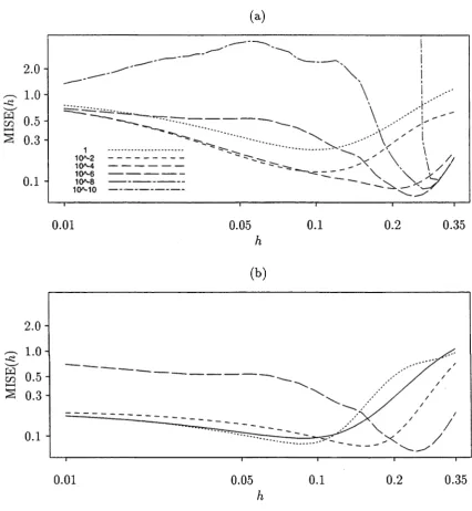
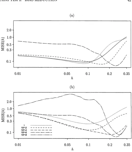
2.6 Numerical Perform ance...33

2.6.1

Comparison with Local Linear E s tim a to r s ... 33

2.6.2

Comparison with Local Cubic E stim ators...38

2.7 Conclusion... 44

CONTENTS

V I

3 L o c a lly P a r a m e tr ic E stim a tio n 48

3.1

Introduction... 48

3.2 Methodology ... 50

3.3 M o tiv atio n s...53

3.4 Theoretical P r o p e r tie s ... 55

3.5 Practical I s s u e s ... 59

4 S k ew in g in D e n s ity E stim a tio n 60

4.1

Introduction... 60

4.2 S k e w in g ...61

4.3 Skewed Estimators and Their P r o p e r tie s ... 63

4.4 Extensions to General Curve E s tim a tio n ...65

4.5 Regularity Conditions

...67

4.6 Technical A rg u m en ts... 69

4.7 Numerical P ro p e rtie s ... 74

5 E s t im a tin g I n te n s ity S u rfaces and C o r re la tio n D im e n s io n s 84

5.1

Introduction... 84

5.2 Correlation Dimension and the Grassberger-Procaccia Procedure . . . 87

5.3 Hill E stim a to r... 89

5.4 Takens Estimator and Binomial E s tim a to r ...91

6 P o le E stim a tio n 94

6.1

Introduction... 94

6.2 Poisson Process P ro p e rtie s...96

6.3 Maximum Likelihood E s tim a tio n ...97

6.4 Nonparametric E stim a tio n ...99

6.4.1

Pole L o c a tio n ... 99

6.4.2

Pole S tr e n g th ... 99

6.5 Estimation of Pole L ine... 102

6.6 Sources of E r ro r ...103

6.7 Large-Sample T h e o ry ... 104

6.8 Numerical S t u d y ...122

6.8.1

Simulated Data without N o ise ... 124

CONTENTS

vii

6.8.3

Kanto Earthquake D a t a ... 132

C h a p t e r 1

K e r n e l R e g re s s io n

1.1

In tr o d u c tio n

N onparam etric regression provides a useful tool for studying relationships betw een covariates and responses in regression analysis. In nonparam etric regression, we re­ move th e restriction th a t th e underlying curve of interest belongs to a pre-determ ined class of functions th a t depend on a finite num ber of param eters. This approach is p articu larly a ttra ctiv e when we have little prior knowledge about th e stru c tu re of the d ata. A dm ittedly, nonparam etric estim ators have zero asy m p to tic efficiency com pared to param etric estim ators when th e tru e model is em ployed. N evertheless, fitting incorrect regression models leads to inconsistent curve estim ato rs, even if we have plenty of data.

Basically, th e form of regression is determ ined by th e m odel in p aram etric re­ gression, and is driven by the d a ta in nonparam etric regression. Because of this, a pre-specified param etric model is often too restrictive to be able to pick up un­ expected features of the regression function. A nonparam etric approach, on th e other hand, provides a flexible m ethod for exploring general relationships between variables. A landm ark exam ple is th e study of hum an longitudinal height growth curves in which the first derivative of the regression function (which corresponds to th e ra te of height growth) is of interest (see for exam ple, Gasser et a/., 1984; R am ­ say and Silverm an, 1997). The nonparam etric m ethod is able to pick up an ex tra peak in th e first derivative which indicates a m id-grow th sp u rt at th e age of about seven. This peak is difficult to detect by ad hoc param etric models, unless one has incorporated this knowledge as p art of th e models. A lthough this exam ple

CHAPTER 1. KERNEL REGRESSION

2

strates convincingly the m erits of nonparam etric regression, it should be noted th a t p aram etric and nonparam etric m ethods are by no m eans m utually exclusive com­ petito rs. Q uite often, it is possible to suggest simple p aram etric relationships from th e nonparam etric analysis. Moreover, in cases where we have inform ation on the form of th e underlying regression function, it proves to be useful to employ non­ p aram etric regression techniques to consolidate or justify our prior understanding of th e curves. See, for exam ple, the m onograph by H art (1997).

T here is now a variety of m ethods for obtaining nonparam etric curve estim a­ tors, some of which are intuitively simple and some m athem atically sophisticated. C urrent nonparam etric techniques employed are m ainly based on kernel functions, splines and wavelets. Recent introductions to kernel and spline approaches may be found in th e m onographs by W and and Jones (1995) and Green and Silverman (1994), and on wavelets in th e paper by Nason and Silverm an (1997). K ernel m eth ­ ods are arguably the sim plest in term s of interp retab ility among th e th ree m entioned m ethods, and we shall review the most relevant ones in Sections 1.2 and 1.3. We shall com pare the N adaraya-W atson estim ator, the Gasser-M üller estim ato r and the local polynom ial estim ator, in term s of their theoretical and practical perform ances. Section 1.4 will discuss some bias-reduction techniques for general kernel m ethods, and Section 1.5 will outline some contem porary devices for guarding against sparse design in local linear sm oothing.

1.2

K ern el E stim a to r s

Unless otherw ise stated , we assume th a t (Ah, Vj ) , . . . ,

( X n, Yn)

are independent and identically d istrib u ted random variables, w ith respective conditional regression m ean and variance given by

m(x) = E ( Y \ X = x)

and

v(x) =

var

( Y \ X

= a :),

C H A P T E R 1. K E R N E L R E G R E S S I O N 3

of m ( x ) can be based on the sizes of these two com ponents. We shall also adopt a com m only-used global m easure of closeness between m and m , m ean in teg rated squared error (M ISE), especially in num erical studies in la tte r chapters. T his is related to MSE by M ISE{m(-)} = J M SE{m(;r)} dx. Unless otherw ise specified, th e term rate o f convergence will m ean pointwise optim al convergence ra te in M SE sense throughout this chapter.

The first kernel estim ator th a t we shall introduce is the Nadaraya- Watson es­ tim a to r friNW (N adaraya, 1964; W atson, 1964), which is based on a local constant approxim ation of m. For each x, is defined as the m inim iser of

^ {Yi — mj v w{ x) } Kh(^— ( E l )

Here, K is called th e kernel function, Kh(') = h ~l K ( -/ /i), and h is known as th e bandwidth. The function K is usually bounded, continuous, sym m etric about 0 and satisfies f K = 1. On m inim ising (1.1), the N adaraya-W atson estim ato r can be given explicitly as

m NW(x) =

E {

K^ X

i~ * ) / E

K h { X ’ ~ * ) } ■

(1-2)

1=1 ^ ' j = l '

It is clear from (1.2) th a t myvw(^) is a local weighted average of th e Vi’s whose weights { I \ h ( X i — x ) / Y^j=i K h ( X j ~ ^ ) } i = i , . . . , n are determ ined by th e kernel func­

CHAPTER 1. KERNEL REGRESSION

4

Bias and variance of

rh^w

admit the following asymptotic approximations:

E{ i nNw{x)

I

Xu . . . , X n} - m(x)

= ^

Kih2

|

m"(x)

var

{rhNW(x) \ X

U . .

. , X n}

= I 1 + °p( i)} » (1-4)

where

K\ = f t 2K( t ) dt

and

«2

=

f K 2.

The deficiencies of

m Xw

are clear from the

bias expansion (1.3) (Chu and Marron, 1991; Fan, 1992). First, the estimator is

biased even when estimating linear functions

m(x) = a + ß x,

due to the presence of

the term

m'(x)f'x ( x ) / f x (x).

Large |

ß

|, or equivalently, large

\m'(x)

| will typically

inflate the bias. Secondly, for non-uniform design where |

f x ( x ) / f x { x )

| is large, the

bias of

ttinw

is also large. Thus, the Nadaraya-Watson estimator is not adequately

design-adaptive.

A better estimator which improves on the bias deficiencies of

rhxw

is the

Gasser-Müller

estimator (Gasser and Müller, 1979), which is given by

71 y » r t I ^

™G

m

(

z

) =

^ 2

{ /

K h(t - x) dt

I

Y

[{],

(1.5)

where {(Aqq, y{t])}i=i,...,n is an ordered sample with ascending

Xßs,

ro = —oo, r n+i =

Too and r z = (Aqq T

X ^ +iß/2.

This approach is based on the approximation

that

f m(t) I\h(t — x) dt

should be close to

m(x)

as

h

—> 0, and is related to the

convolution smoothing introduced by Clark (1977). Clark suggested convolving a

piecewise-linear estimator

g

with a kernel function

K

, and proposed the estimator

rrtCL{x)

g{t) I\ h(t — x ) d t ,

where

g

is simply a first-order interpolating spline defined by

(1.6)

r yji]

for

t < x {l)

,

9(t) — \ ^[*] + x (['+1)1 -v /.j (* — * « ) ^or ^(*) - i - ^(*+i) (* = 1, • • •, n — 1 ),

1

Y[n\

for

t > X{n) ■

C H A P T E R 1. K E R N E L R E G R E S S I O N 5

1990). The conditional bias and variance of th e Gasser-M üller estim ato r are ob­ tained as

E { r h GM(x) I X i, . . . , X n } - m( x ) = \ Kxm"(x) h 2 {l + op( l) } , (1.7) vai { m GM { x ) \ X 1, . . . , X n } = § { nh f x ( x ) } ~ 1 n 2v( x) { l + op(l)} .(1 .8 ) The bias of th e Gasser-M üller estim ator, which is independent of th e design density f x and depends only on the curvature of m , has a sim pler representation com pared to th a t of th e N adaraya-W atson estim ator. It is also easier to in terp ret, since for large local curvature, | m"( x) | tends to be large and we should expect m ore bias to be introduced. The asym ptotic variance of iriGM, however, is 1.5 tim es th a t of rhjxw in the random design m odel (com pare (1.4) and (1.8)). Seifert and Gasser (1996b) used a pictorial illustration to dem onstrate why the variance is inflated: if th ree design points are close together, the m iddle point receives much less weight com pared w ith th e other two points since the weights of th e response variables are proportional to th e areas under th e kernel function between averages of subsequent design points. The Gasser-M üller estim ator assigns fluctuating weights to th e response variables and increases variability. Several m ethods have been proposed to alleviate this problem- they include works by H errm ann (1996) and Hall and T urlach (1997a). These m ethods focus on choices of r t-’s (at (1.5)) th a t reduce th e variability of th e weights.

1.3

L ocal P o ly n o m ia l F ittin g

CHAPTER 1. KERNEL REGRESSION

6

Specifically,

iriLp{x)

is given by

ß0,

where

ß =

(/?0, . . . ,/?p)T is chosen to minimise

V 2

Y . - J 2 0 J (Xi

-

[

K h{Xi - x

) .

(1.9)

t = l ^ jr = 0

This minimisation problem can also be put in matrix form as follows (Ruppert

and Wand, 1994). Denote

1 X i - x .. ■

(X, -

\

(

Yl

\

X =

,

Y =

\ 1

X n - ..■ (Xn ~ X)” )

\ Y n J

and

W

= diag

{Kh{X

i — x ) ,. . . ,

I \ \ ( X n

— a;)}, the

n x n

diagonal matrix of weights.

Assuming the invertibility of

X TW X,

the solution of the least-squares problem (1.9)

can be rewritten as

ß

=

(X

t

W X )"1X t W Y ,

(1.10)

and

rriLp(x

) =

e Tß

where

eT

= ( 1 ,0 ,...,0 ) is a

(n +

1)

x

1 vector. For

p =

0,

the local constant estimator obtained from minimising (1.9) is equivalent to the

Nadaraya-Watson estimator (1.2). For p = 1, we obtain the local linear kernel

estimator

n

^

ll

(

z

) = (s0s2 - s?)-1 ^ {s2 -

{Xi -

x)si}

K{ ( Xi

-

x)/ h} Y

t ,

(1.11)

2 — 1

where

s r = i ^ i

—

XY X { ( X i — x ) / h } ,

r —

0,1,2. An equivalent expression for

mLL(x) is

friLL = (1.12)

where

Wi =

{s2 — (Xt- — x )si}

K{(X{ — x)/h}.

The theoretical properties of local

linear fitting and polynomials of other orders have been well-studied (Fan, 1992,

1993; Ruppert and Wand, 1994; Fan

et

a/., 1997). We shall only detail properties

in the local linear case. The conditional bias and variance of

tull

are

=

\ K i m ”(x) h2

{ l + op(l)} ,

K:

M

X) f l , .

E { m LL(x)

var

{ m LL(x) \ X u . . -, X„}

(1.13)

C H A P T E R 1. K E R N E L R E G R E S S I O N

7

Fan (1993) showed th a t the globally optim al bandw idth w ith respect to integrated conditional m ean squared error is

in th e sense of asym ptotically minimising MISE. B oth th e local linear estim ato r and th e Gasser-M üller estim ator have th e same asym ptotic bias, b u t th e asym ptotic variance is sm aller for th e local linear sm oother and is th e sam e as th e N adaraya- W atson estim ato r in th e random design setting. Hence, is superior to th e two kernel estim ators introduced in the last section, in term s of bias and variance. It is w orth m entioning th a t th e degree of th e local polynom ial, p, determ ines th e size of bias of rriLp(x) which decreases as p increases (R uppert and W and, 1994). However, the practical gains of high degree fits are doubtful for th ree reasons: (i) it is com putationally costly to solve the m inim isation problem (1.9) for large p, (ii) th e inversion of X TW X in (1.10) m ay create num erical instability in regions w ith sparse design, and (iii) the variance of ttilp is inflated for higher degree fits and a large sam ple m ay be needed for practical im provem ents. For these reasons, one rarely uses local polynomial fits w ith p > 3. See Section 1.4 for m ore discussion of higher order polynom ial fits.

The advantages th a t ttill offers are more th an merely those m entioned above. W hen th e design density f x has bounded support, say on th e closed interval [a, 6], a regression sm oother using com pactly supported kernel norm ally behaves differently when it reaches a boundary and has slower ra te of convergence. We call points lying in th e interval [a + h, b — h\ interior points, and those lying outside this interval boundary points. For th e N adaraya-W atson and th e Gasser-M üller estim ators, bias increases by an order of m agnitude to 0 ( h ) in estim ating boundary points, hence optim al MSE inflates from th e usual order n ~4N to n -2//3 (Rice, 1984; Gasser and M üller, 1989). W hile this is only a theoretical result, th e boundary effect is, in practice, quite noticeable (H astie and Loader, 1993). To cope w ith boundary effects, a popular m ethod is to employ special boundary kernels (Müller, 1984, 1991; Jones, 1993) which typically have th e form

where a and ß are determ ined by m om ent conditions. A lthough this m ethod solves th e problem of boundary effects, it offers no intuitive in terp retatio n and is arguably

(1.15)

C H A P T E R 1. K E R N E L R E G R E S S I O N

8

too artificial. O ther m ethods for correcting boundary effects include extrapolation m ethods (Rice, 1984) and reflection m ethods (Hall and Wehrly, 1991).

Local linear regression, on the other hand, requires no m odification when esti­ m ating th e boundary (Fan and Gijbels, 1992). Bias and variance at th e boundary rem ain autom atically th e sam e order as in th e interior. Indeed, since local linear approxim ation is used in a sm aller interval, the bias at a boundary point is sm aller th an th a t at an interior point. On th e other hand, variance increases at a boundary point since fewer d a ta points lie in th e interval. Note th a t this au to m atic bound­ ary bias correction is only available for local polynom ials of odd degree (R uppert and W and, 1994). Thus, in d ata analysis, one norm ally uses local linear or cubic sm oothers.

A nother a ttra ctio n of th e local linear sm oother comes from a more m ath em atical view point, mini max risk analysis. This gives a m easure of how well one estim ato r perform s com pared w ith another under specific functional criteria on th e class of estim ators and th e underlying regression function. Define a linear smoother as:

The N adaraya-W atson estim ator, th e Gasser-M üller estim ato r and th e local linear estim ato r are clearly linear sm oothers from this definition. Denote

C2 = { m : I m ( x ) — m ( x 0) — m ' ( x 0)(x — x 0) | < C (x — xq)2/ 2 } , where x 0 is an interior point. Assume also th e following conditions:

(i) u(-) is continuous at th e point rro,

(ii) f x { ’) is continuous at th e point x 0 w ith f x ( xo) > 0 • The linear mini max risk is defined as

and the best linear sm oother is the one which achieves this linear m inim ax risk. Fan (1992) showed th a t th e local linear estim ato r ttill w ith th e Epanechnikov kernel,

I \ e, and bandw idth, h0 given by

n

rhL{x) = ^ 2 W i ( x , X i , . . . , X n) Y i.

C H A P T E R 1. K E R N E L R E G R E S S I O N 9

achieves th e linear m inim ax risk. In other words, the linear minimax efficiency of

t t i l l-, defined by

________________R L(n, C2)________________ supmec7 E [ { r h LL( xo) - m(:ro)}2| X u . . . , X n\

5 / 4

(1.16)

is 100% am ong all linear sm oothers, in an asym ptotic sense. N ote too th a t th e N adaraya-W atson estim ato r has asym ptotic linear m inim ax efficiency 0 since its bias (1.3) depends on th e derivative m'(xo) and its m axim al risk is infinite over th e class C2- T he Gasser-M üller estim ator, w ith a larger variance com ponent com pared w ith t t i l l-, is only 66.7% as efficient as t t i l l• Fan (1993) extended this result and

proved th a t on im posing additional restrictions on th e jo in t density / , th e m arginal density f x and the conditional variance u, m inim ax efficiency (defined as in (1.14) bu t dropping th e constraint in Rl(j i->C2) th a t m i is a linear sm oother) rem ains at 89.4% am ong all estim ators.

Assume now th a t th e design density has bounded support. Do the appealing m inim ax ra te properties of t t i l l extend to estim ating boundary points? T he answer

is affirmative. Cheng, Fan and M arron (1993) showed th a t th e local linear regression estim ato r achieves 94.4% linear m inim ax efficiency in estim atin g the left or right boundary point. Thus, ttill is nearly optim al in estim ating th e boundary am ong all linear sm oothers. R esults of m inim ax efficiency on local polynom ials of other degrees, and on estim ating derivatives, are discussed in detail by Fan et al. (1997).

1.4

B ia s -R e d u c tio n M e th o d s

In this section we shall review bias-reduction techniques applicable to general kernel regression m ethods. By reducing the order of m agnitude of bias, one obtains rates of convergence b e tte r th a n th e usual n~4l5. In th e next chapter, we shall introduce a new bias-reduction m ethod in local linear sm oothing.

Higher-order kernels were noted by B artle tt (1963) in th e context of probability density estim ation. We call K a j - t h order kernel if it satisfies

J

K — 1 ,

J

t 1 I \ ( t ) dt = 0 for i = 1 , . . . , j — 1, and

C H A P T E R 1. K E R N E L R E G R E S S I O N 10

m om ents. A general j -th order kernel sm oother has th e form

2 — 1

where K(3) denotes a kernel of order j . To see why higher-order kernel techniques can reduce bias, we note th a t the conditional expectation of m ( x ) is

E { m ( x ) \ X i, . . . , X n } = j ' K(j)(u) m ( x + uh) du .

Assuming sufficient regularity conditions, m ( x + uh) m ay be expanded as a Taylor series about x and the m om ent conditions on K(j) ensure th a t th e bias of rh(x) is of order hJ. Notice th a t higher-order kernels take negative values, and th a t the overall perform ance of m( x ) m ay be undesirably affected. It is m ore difficult to in terp ret th e resulting estim ato r when negative weights are assigned to some of the Yi's. In th e related context of kernel density estim ation, use of higher-order kernels may even result in a negative density estim ate.

As m entioned in th e previous section, th e degree of th e local polynom ial d eter­ mines the order of bias of th e estim ator ttilp• R u p p ert and W and (1994) showed th a t for local pth-degree polynom ial fits, conditional bias adm its the following formulae:

E { m LP( x ) \ X i , . . . , X n } hp+' f m

(p+i)

1 (p +~ j! } { /

uP+l K\

p

](u) du]

I 1 + °p( 1)} if p is odd ,

if p is e v e n , (1.17)

CHAPTER 1. KERNEL REGRESSION

11

Another bias-reduction method was given by Härdle (1986) using a

jackknife

technique. This approach is very similar to that proposed by Rice (1984), who

combined two kernel estimators to reduce boundary bias, which was motivated by

Richardson extrapolation. Let m^(ar) be a kernel smoother with bandwidth

hj

which admits asymptotic bias

C( K) m"(x) hj

(see (1.7) and (1.13)) for

j =

1,2, and

C( K)

is a constant which depends only on

K

. The jackknife estimator is given by

rhj(x) =

(1

-

lo

)~1 { m hl(x) - u > mh2(x)}

,

and has asymptotic bias given by

b(x) =

(1 — a;)-1

(h\ —ujh\) C( K) m"( x

), provided

uj

^

1. The choice of

to

is crucial here, since

b(x) =

0 if

u

is taken to be

h\ /h\ .

Hence, the bias of

rhj(x)

is reduced compared with

rhh^x)

or

rhh2 (x).

Note that

rhj(x)

is equivalent to the kernel smoother based on the kernel

L(

u

,

uj

)

= (1 —

lj

) { K (

u

) —

to3/ 2

K(ujlt2u)},

with

La

— h\ /h\ ,

where it may be easily shown that

L(

u

,(

jj

)

is a fourth-order kernel. Thus, jackknifing is essentially a high-order kernel

method. A comparison of efficiency of the jackknifed kernel smoother with respect

to ordinary kernel estimators can be found in Härdle (1986). In practice, one has

to jointly select

hi

and

uj

(or equivalently,

hi

and

h

2), and the performance of

rhj

seems to be fairly sensitive to the choice of

lj

.

Variable bandwidth bias-reduction methods were introduced by Breiman, Meisel

and Purcell (1977) and Abramson (1982) in the context of density estimation. In­

stead of choosing a constant bandwidth over the entire range of inference, the band­

width is allowed to vary and depends on the data. In nonparametric regression, a

kernel estimator of

m(x),

with variable bandwidths

hi/oti(Xi)

in the numerator and

h2/ a 2(Xi)

in the denominator, is given by

~

,

(n

h

) - 1

i

EL,

«

i

(V.)

K

{

-m v B ( X ’

where

K

is assumed to be a second-order kernel. Hall (1990) studied the bias

of a variable bandwidth estimator in very general settings and showed explicitly

how to determine appropriate cq and a 2 for minimising bias. He recommended,

C H A P T E R 1. K E R N E L R E G R E S S I O N 12

respectively, where /i3, h4 are bandw idths of size n -1 / 5. The “adaptive form ” esti­ m ato r, rhvB, defined by sub stitu tin g ctj for ctj in rhvB-, preserves th e bias-reduction qualities of rhvB w ithout appreciably affecting variance. Though this m ethod is capable of reducing bias, its com plicated n atu re makes it less appealing in practice.

The m ultiplicative bias-reduced estim ator (M BRE) for n onparam etric regression was proposed by Linton and Nielsen (1994). It has m ean squared error of order n~8/9. The idea is relatively straightforw ard. An initial sm ooth, say m (;r), is obtained. W rite m ( x ) = a ( x ) m ( x ) where q(x) = m ( x ) / m ( x ) . The M BR E is defined as i ti mb{x) = a( x) f h( x) , and a( x ) is an estim ate of a (x ). By suitably choosing a ( x ) it is possible to reduce bias from size h2 to h4. Linton and Nielsen (1994) tre a ted only th e case for equispaced design. Jones, Linton and Nielsen (1995) proposed a more generally-applicable version by employing the local linear estim ato r tull^ ) as th e initial sm ooth, and m ultiplying this by a local linear regression of Yi/rriLL(Xi) on Afi. To be explicit, they defined their estim ator as

n

friMB(x) = rnLL(x)

i=l

K { ( X j - x ) / h } ( Yj i (s0s 2 - s l ) '-rhLL(Xi)> '

where 5t-’s are defined as in (1.11). Jones, Linton and Nielsen (1995) showed th a t th e bias of this estim ator is of order /i4, while th e variance rem ains th e sam e order { nh)~l .

1.5

O v erco m in g Sparse D e s ig n

CHAPTER 1. KERNEL REGRESSION

13

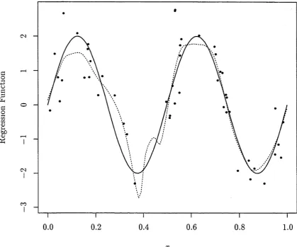
Figure 1.1: Local linear kernel estimate for the regression function m(x)

= 2 sin 4

ttx

with sample size n =

50. The solid curve is the true regression function, and

the dotted line is the local linear kernel estimate. The Standard Normal kernel

is employed, and the bandwidth

h =

0.0335 is chosen to minimise the asymptotic

MISE.

section, the local linear smoother will be denoted by m, and we assume the kernel

used to construct

m

is compactly supported on [—1,1].

[image:21.536.74.494.119.468.2]

CHAPTER 1. KERNEL REGRESSION

14

and Gasser suggested that this can be done in two steps. First, compute the finite-

sample variance

Vh0{rn(x

o)| A fi,...

, X n}

and compare it with some reference level,

say

8 VhQ,

where

8

is a pre-specified constant, and I40 is the asymptotic variance

(1.14) calculated for uniform design. When

Vh0{rh(xo) \ X \ , .

. . ,

X n )

exceeds the

reference level

8\

4 0, the bandwidth is locally increased. It may be that, however,

an increase in bandwidth does not result in a sufficient decrease in variance. In this

case, variance-bias consideration comes into play. As the bandwidth increases from

ho

to

the asymptotic squared bias increases in proportion to

( h i /h 0)4.

Thus, as

a second step, one finds

h

to minimise

Vho{m(x

o ) |* 1, . . . , V n} + ( - A - ) 4 ^ .

(1.18)

Extension to local polynomials of other degrees, as well as further arguments that

lead to minimising (1.18), can be found in Seifert and Gasser (1996a). They also

showed, through simulation studies, that the choice of

8 =

1.0 behaves well.

Another method introduced by Seifert and Gasser (1996a, 1996b) is to incor­

porate a parameter, known as a “ridge”, in the estimator. Recall that in (1.10),

calculation of

ß

involves the inversion of X TW X . In regions of sparse design, this

matrix is close to singular or even non-invertible. Ridging guarantees that this ma­

trix is non-singular, through the addition of a positive semidefinite matrix

H

such

that

H

+ X TW X is non-singular; and the ridged estimator is given by

ß = (H

+ X

t

W X )" 1X t W Y .

The principle involved in ridging has in fact been adopted by Fan (1993) in proving

the optimal performance of the local linear smoother. He defined the local linear

smoother (1.12) slightly different by adding a factor of

n~2

to the denominator :

iri(x)

(1.19)

This has the effect of avoiding zero in the denominator when there are no design

points in the interval X =

[x — h, x + h].

Seifert and Gasser proposed several choices of

C H A P T E R 1. K E R N E L R E G R E S S I O N 15

together w ith th e bandw idth, and th e perform ance of the estim ato r can be seriously im paired by a poor choice of th e ridge param eter. We shall d em o n strate this in the num erical section in th e next chapter.

A nother technique, form ulated by Cheng, Hall and T itterin g to n (1997), involves shrinking a local linear sm oother towards a general curve estim ato r, m. Indeed, ridging described in th e above paragraph can be viewed as shrinking rh towards 0. Recall th a t in local linear sm oothing, one chooses a and b to m inim ise

- « - & ( * , - * ) } 2 A ' ( ^ ^ ) ,

(1.20)

and m is defined by a. In shrinkage, th e expression at (1.20) is generalised, and one looks for a and b to m inim ise

{Yi — a — b(X{ — x ) Y K ( “ T - “ ) + 6 {rä(rr) — a } 2 , (1.21)

where t = e(x) > 0. T he new estim ator, m s, is taken as a in th e m inim isation of (1.21) and can be given explicitly as

m s W{ Y{ + e $ 2r n j w t + e s 2 j ,

i=1 /

(1.22)

where Wi and s 2 are defined as in (1.12). Taking m = 0 and t = ( n 2S2) _1 in (1.22) gives th e ridged version of th e local linear sm oother (1.19). Note th a t rhs = rh when e = 0, and rhs = rh if e = oo. Cheng, Hall and T itterin g to n (1997) suggested taking m to be another local linear sm oother, constructed using th e sam e bandw idth but w ith an infinitely supported kernel to guard against th e sparse-design problem . The advantage of this approach is its ability to produce a proper curve estim ato r even when an excessively large shrinkage param eter is chosen. This was supported both in the theoretical and num erical studies by Cheng, Hall and T itterin g to n . Moreover, rhs can be regarded as a “m ix tu re” of two local linear estim ators using com pactly and infinitely supported kernels respectively, and enjoys th e m erits of reduced edge effect and lower m ean squared error (if th e Epanechnikov kernel is used) from the form er, and increased num erical stability from th e latter.

C H A P T E R 1. K E R N E L R E G R E S S I O N 16

th e kernel and the bandw idth used to construct the local linear estim ato r. The m ethods are applicable to all bandw idths, and are easy to im plem ent. Indeed, using a suitable interpolation rule allows th e conditional m ean squared error of a local linear sm oother to be stated in an unconditional sense.

Assume th a t the random sam ple {(A ;, K ) } i = i , . . . , n has its predictor variables As­

sorted in ascending order, i.e. X \ < . . . < A n; th a t th e kernel K has support on [—1,1]; and th a t the A ;’s lie in the com pact interval [a, 6]. P u t (Ao,Vo) = (a, IS) and (A n+i, Yn+i) = (b, Tn), and let Si = A ;+i — X t for 0 < i < n. Let J h denote the set of indices i such th a t a + h < X t < A t+i < b — h, where h is th e bandw idth used in th e local linear estim ator. For a given real num ber r, w rite m; for th e integer p art of r S i / ( 2 h ) if i £ j7h, and for th e integer p art of r S i / h otherw ise. If m z- > 1, add rrii equally-spaced pseudo design points to the interval [A,-, A,-+i]. For each pseudo point, th e corresponding Y-value is generated by linear interpolation betw een the points (Aj-,1S) and (A t+1,Vi+i). Essentially, the interval [At-,A t-+i] is divided into m l -f 1 equal portions of length not exceeding 2 h / r if i G J h , and h / r otherw ise. If m l = 0, no pseudo design point is added. This rule ensures th a t none of th e distances between two adjacent design or pseudo points is more th a t 2h / r . Equivalently, for each x € [a, 6], th e num ber of those points in the interval (x — h , x + h) is a t least equal to th e integer p a rt of r.

C H A P T E R 1. K E R N E L R E G R E S S IO N 17

[image:25.536.70.495.128.484.2]

CHAPTER 1. KERNEL REGRESSION

18

1.6

S u m m a ry

This chapter highlights some favourable properties of local polynomial estimators.

The local linear estimator, in particular, enjoys excellent numerical as well as theo­

retical properties (e.g. Fan, 1993; Hastie and Loader, 1993; Cleveland and Loader,

1996). Among all linear estimators, it is 100% efficient in estimating regression

means with two bounded derivatives, and nearly 90% efficient among all estimators

in an asymptotic minimax sense (Fan 1993). Widely-used smoothing software is

C h a p te r 2

B ias R e d u c tio n

2 .1

I n t r o d u c t io n

The favourable properties of local linear smoothing were discussed in the last chap­

ter. For regression functions that exhibit a high degree of smoothness, local poly­

nomial methods of higher order are, at least in theory, superior to local linear ap­

proaches in reducing bias, as mentioned in Section 1.4. Nevertheless, higher-degree

fits require necessarily more elaborate techniques for guarding against data sparse­

ness problems, compared to those for local linear smoothing. For example, to obtain

a local cubic estimator, one needs to invert a 4 x 4 matrix (see (1.10)) and to avoid

numerical problems in regions where the design is sparse, one has to ensure that this

matrix is not close to being singular.

In this chapter, we shall demonstrate how one may achieve bias reduction by

combining two or three linear estimators, obtaining essentially the same optimal

performance as the local cubic smoother. The techniques employed by local linear

estimators to guard against data sparseness problems may be applied directly to

our new estimators. Essentially, our method involves a convex combination of local

linear estimators with easily-chosen weights that depend only on the kernel function,

and not at all on other unknowns like the regression mean or design density. It has

similar spirit to the bias-reduction methods introduced by Schucany and Sommers

(1977) and Härdle (1986), who suggested using a linear combination of two kernel

estimators of different bandwidths, and has already been discussed in Section 1.4.

Figure 2.1 demonstrates a simple graphical property which motivates our method.

The true regression mean is convex, and the standard local linear estimator tends

CHAPTER 2. BIAS REDUCTION

20

[image:28.536.101.459.114.417.2]

x — Ih x x + lh

Figure 2.1: Bias reduction via a convex combination of three local linear smoothers.

By choosing the weights in an appropriate way, bias contributions from the two

asymmetric smooths on either side of the symmetric smooth will cancel those of

the latter, resulting in reduction of bias by two orders of magnitude. For a slightly

different choice of either of the asymmetric smooths, the line segment will cut the

curve at a point whose abscissa is very close to x, and so reduce bias by one order

of magnitude.

re-C H A P T E R 2. BI AS REDUre-CTI ON 21

move all th e first- and second-order effects of bias. In fact, as we shall show later, this reduces bias by two orders of m agnitude com pared w ith stan d ard local linear sm oothing. Variance may be reduced, although only by a constant factor, not an order of m agnitude. The am ount of variance reduction depends on the kernel type.

Using a single local linear estim ator calculated in a slightly asym m etric way, bias and variance have th e same order as for a local q u ad ratic sm oother. This approach m ay be m otivated by considering the construction of th e local regression line so as to ensure th a t the expected value of the place where th e line crosses th e curve has its abscissa very close to the one at which we wish to estim ate th e curve. To a significant extent this m ay be guaranteed w ithout prior knowledge of th e curve. T he average of two of these sm ooths, on either side of the point at which we wish to estim ate th e regression mean, reduces bias by two orders of m agnitude. Indeed, this average can be viewed as a lim iting form of the estim ato r described in th e paragraph above. We shall term our technique “skewing” , which reflects th e use of asym m etric m ethods to im prove perform ance.

This chapter is organised as follows. Section 2.2 introduces a general version of th e skewed estim ators, and Section 2.3 presents m ain theoretical properties. Left- and right-skewed estim ators are introduced in Section 2.4. Section 2.5 discusses general issues and extensions to our skewing m ethods. N um erical perform ance is addressed in Section 2.6. There, we show th a t a simple interpolation device (Hall and Turlach, 1997b), borrowed from the case of ordinary local linear sm oothing, m ay be used to guard against sparse design.

2.2

G en era l Skew ed E stim a to r s

C H A P T E R 2. B I A S R E D U C T I O N 22

pair (a, b) is obtained by m inim ising

n

J 2 { Y , - a - b ( X , - x ) } 2 K h(Xi - x) ,

z = 1

where Kh{' ) = h ~ l K ( - / h ) and h is a bandw idth. The m inim ising pair (a, b) depends on x as well as on the d ata, and is denoted by { a( x) , b( x) } . E lem entary calculus shows th a t the m inim isers are

a(x) = r 0( x ) s 2(:r) - r i ( z ) s i ( ; r ) b(x) = r 1( x ) s 0{x) - r0( x ) s i ( x ) s0( x ) s 2( x ) - s i ( x ) 2 1 ' 50(a;) 62(a:) - 5 i(x )2

where r t(x) = Yn=i - x ) 1 K h{Xi - x) Yi and si(x) = (Xi ~ x )l K h ( X t - x),

l = 0,1,2, . . . .

T he estim ato r of the line y = y(u) is m( u \ x ) = a(x) + 6(x) (u — ar), w ith form ula r0(x) s 2{x) — r i (x) 5i(a;) + { ri(a ) 50(x) - r 0(x) 5i(x)} (u - x)

rh(u\x) — (2.1)

s0( x ) s 2(x) - s i ( x ) 2

The stan d ard approach to local linear regression involves fitting a straight line segm ent whose m idpoint is directly above th e point x a t which we wish to es­ tim a te th e curve. P u ttin g u = x in (2.1) gives th e usual local linear estim ato r m ( x ) = m ( x \ x ) = h(x), which has conditional bias of size h2 and conditional vari­ ance of size (n h )-1 (Fan, 1993). Skewing involves fitting th e straight line segm ent in an asym m etric m anner, w ith its centre a little to th e left or right of x. A general skewed estim ato r m is a convex com bination of three local linear sm oothers

\ i i ri (x\ x + Uh) -f m ( x \ x ) + \ 2m ( x \ x T l2h)

s(x) =

Ai T 1 + A2 (

2

.

2

)

where A1? A2 > 0 are weights, l\ < 0 and l2 > 0. Versions of (2.2) will be described in Section 2.4. Intuition suggests th a t we take Ai = A2 = A and C = —12 = /, say, so as to enhance th e sym m etrical stru ctu re of rh(x) and reduce bias. In fact, this choice is necessary if we want to reduce bias by two orders of m agnitude. Theorem 2.1 in th e next section shows this explicitly. The theorem also shows th a t the param eters A and / are related by a sim ple relation which depends only on th e kernel function.

2.3

T h e o r e tic a l P r o p e r tie s

CHAPTER 2. BIAS REDUCTION

23

T h e o r e m 2.1

Assume that m has four bounded, continuous derivatives in a neigh­

bourhood of x; that f has two bounded, continuous derivatives there and f ( x )

> 0;

that the kernel K is non-negative, bounded, symmetric and compactly supported,

with f K

= 1;

and that h = h(n) —>

0

and nh —>

oo.

Take X\

=

\ 2

= A > 0

and

1

1 = —

l2

= /( A),

where

l(

A) = { ( 1 + 2 A )k2/(2 A )} 1/2. (2.3)

Then the bias of rh is given by

E{m(x) —

m ( x ) |X i ,. . . , X n} =

B(x) h4

+

oP{h4

+ (n /i)-1 / 2} ,

where

B(x) =

{16 /(ar)} _1 [2{2

f"(x) m"( x)

+

4 f'(x) m"' (x)

+

f ( x ) m ^ v\ x ) }

x («2 — «4) —

X~l K,lf(x)

.

R e m a r k 2.1 . The theorem actually holds under weaker sym m etry conditions th a n those im posed on

K.

In particular, we require only « 1 = « 3 = 0, not sym m etry. Hence we shall retain term s in /c5 in our proof below.

R e m a r k 2.2 . It is, in fact, not necessary to assum e th a t a skewed estim ato r has the form

rh(x\x

±

k)

where

k

=

Ih.

The fact th a t

k

is of size

h

m ay be deduced directly from th e proof.

P r o o f o f T h e o r e m 2 .1 . P u t

fi(u\x)

=

E { m ( u \ x ) \ X \ ,

. . . ,

X n},

which we m ay expand as

fi(u\x)

=

m( x) + (u — x)m' (x) + {<s0(a:) s2(x) — ^ i( ^ ) 2 } - 1

(Q(^)

+ -R(a;)} , (2.4)

where

Q(x)

equals

\ m"(x)

[{s2(2?)2 - 53(x) 5i(x)} + (u

-

x) {5 3(2:) 5 0(2:) - 52(2:) 5 1(2:)}] + |

m'"(x)

[ { s 3 { x) s 2(x)

-

5 4(2;) Si (x)} + (u - x) {^4(2r)^0(x) - s 3(2:).si(2:)}] + T

m (lv\ x )

[{<s4(2?)

s2(x) - s5(x)

6 1(2:)} +

(u -

x) ( s 5(x )s 0(x) - s4(2:)s i(2:)}] ,

(2.5) and R (x ) may be expressed concisely using an exact form ula for th e rem inder in Taylor’s theorem . It m ay be easily shown th a t

C H A P T E R 2. B I A S R E D U C T I O N 24

where Z/ is a random variable which is asym ptotically norm ally d istrib u ted , w ith m ean 0 and variance f ( x ) f u 21 K ( u ) 2 du. It follows from Taylor expansion th a t

( n h l+1) ~ l si(x) = ki f ( x ) + Ki+1 f ' ( x ) h

+ \ ki+2 f " { x ) h 2 T °{h2) + Op{ ( n h ) 1//2} . (2-6) Let 7/ and Si denote generic positive num bers which equal o(hl) + 0 { ( n h ) ~ 1/ 2} and o(hl) + 0 { h 2 (n h )-1 / 2} respectively, and define r^i(x) = Sk(x)si (x) — Sk+i-i{x)si(x). T hen, using (2.6), we m ay obtain:

n 2h 4 r0 2(x) 1

n 2h 6 r 22(x) n ~ 2h ~5 r30(x) n ~ 2h ~ ‘ r 32(x) n ~ 2h~6 r 40(x) n ~ 2h~s r 42(a:) n ~2h ~ ‘ r 50(x)

_ 1 ___ f ( x ) 2K2

{ f ( x ) k2} 2 + { / " ( x ) f ( x ) - f ( x)2} k2k4 h 2 + op(72), f ( x ) f ' ( x ) («4 - k\) h 2 + i /(a;) /" ( x ) k5 h 2 + op(72),

- 2 / ' ( a : ) 2}/c2«5 h 2 + op(72),

/ ( z ) 2 /c4 + / ( x ) /'( x ) «5 h + op( 7 i ) , / ( x ) 2 k2k4 + op(70),

/ ( x ) 2 K5 + Op(70) .

Defining tki(x) = r 02(x) 1r ^ ( x ) , we may deduce th e following formulae:

122

^30 ^32 t 42

K2h 2 T

—

fx

2) fi

4

+ Op(^4) ,

/ 7(x) (k4

-/ (x)k2

Op(^4) ,

AC4/l4 + Op(J4) ,

h

2

+ Q x U ,

A3 + s ) ;

2 /( x ) «2

<40 = - A2 + *3 + o p(<53) , « 2 / (Z) « 2

^50 — ---- + O p (<^3) .

«2

CHAPTER 2. BIAS REDUCTION

25

may prove that for any fixed /,

jj.(x\x

+

Ih)

=

m(x)

+ | (

ac

2 —

l2) m"(x) W

+ l f

-

«<)

2

1

f{x)*2

' /"(*)

2 /(l)

1

+

2

m"(x) + ( K2 “

"

t

) m'"( l) } fcS

/

2N

U"{

x

)

k

5

\

f { x )

/ I

4

2j

2/ ( * )

k

2

+

/"(®)

Z'

f ' ( X) Y

I

/ 2 ( ^ 2

- «

4

)

x /(* )

\ / ( * )

//'(rc) {3/ («2 - «4) ~ ^5}

« 2

m ”(x)

3f(x)K2

m'"(x)

+

1 f «4 /«5 , /2( 3 ^ - 2 / C 4) (iv), ^ L4 ,

2 \ y - ^ + —

3 ^ —

2 r

(x), T + 0 ^ 4)

-(2.7)

Considering versions of this formula in the cases / = 0,

l\,

Z2? and combining them

to produce a formula for conditional bias for

fh(x)

defined at (2.2), we see that the

terms in

h2

and

h3

vanish if and only if

Ai(«2 — Y ) + k 2 + A2(k2 — l \ ) — 0 ,

A

1/1

A2/2 = 0,

A

1

+ A2/^ — 0.

Assuming only that Ai, A2 > 0 and /j,

l2 ^

0, the latter two equations imply that

\ x —

A2 = A and

l\ = —l2

= /, say. The first equation then gives

l =

/(A), where

/(A) is defined by (2.3). Finally, the claimed bias expansion in Theorem 2.1 follows

directly from (2.7).

Asymptotic properties of the conditional variance of m can be derived similarly,

and are given in the next theorem.

Theorem 2.2 Assume the conditions imposed on K and h in Theorem 2.1, that f

has a bounded derivative in a neighbourhood of x, and that v(u) —

var

{Y\X

=

u) is

bounded and continuous there. Assume that

=

A2 = A > 0

and 1

1

= — /2 = /(A).

Then,

C H A P T E R 2. B I A S R E D U C T I O N 26

where

V(A) = (2A + 1)“ 2 (2 A2 + 1) j K ( u f d u

+ (6A + 1) j K ( u — l ) K ( u ) d u

+ i(4 A + l ) 2

J

K ( u - l) K ( u + l) du

+A(2A + 1)^2 1

J

u2{ K (u) 2

-

K ( u - l)

+ /)}

di . (2.8)

P r o o f o f T h e o r e m 2 .2 . Since X i = A2 = A > 0 and = — l 2 = /(A), th e estim ato r

at (2.2) may be expressed as

m( x ) = (2A -f l) 1{Am(x|a: + Ih) + m ( x \ x) + rh(x\x — /h)} . (2-9) D enote th e conditional variance of m (n |x ) by i){u\x), and the conditional covariance of m (n|;r) and m( u\ y) by c(u\ x, y). T he conditional variance of th e regression m ean m ay be w ritten as

var {m(x)\ X i, . . . , = (2A + l) 2{A2 fj(x\x + Ih) + rj(x\x) + A2 i)(x\x — Ih) +2A c{x\x — l h , x ) + 2A c(rr|x, x A Ih)

+2A2 c{x\x — //i, x + Ih) } . (2.10) Up to first order, Theorem 2.2 follows from expansions for each term on th e right- hand side of (2.10). For the sake of brevity, we shall only give details for th e ex p an ­ sion of fj(x\x -f Ih). O ther term s may be expanded by following sim ilar argum ents as below. Using the definition of m( u\ x ) at (2.1), we m ay express

fj(x\x A Ih) = E [{d(x + Ih) — Ih b(x + l h ) } 2\ X\ , . . . , X n]

- [ E { a ( x + Ih) - l h b ( x + l h ) \ X u . . . , X , } ] 2

= var {a(x + Ih)| X\ , . . . , Xn} + (Ih)2 var {b(x A Ih)| X i, . . . , X n } —2 Ih cov {a(x A Ih), b(x A lh) \ X\ , . . . , Xn}

= Tx -f T2 — 2 T3 .

Form ula (2.6) in the proof of Theorem 2.1 gives the following identities: s0(x) = n h f ( x ) { l + Op (1)} , Si(x) = n h 6 f ' ( x ) t i 2 { l + oP(l)} ,

C H A P T E R 2. BI AS REDUCTI ON 27

whence it follows th a t

So(z) <S2(ar) — 5i(a:)2 = n 2h4 f ( x ) 2 tz2 { l + op(l)} .

From th e definitions of ä and b together w ith (2.11), we deduce th a t

n

{*< - (x + h h ) } u { X, - (x + l2h)} ‘2

(

2

.

12

)

2= 1

x K

X{ — (rr 4- l\h) 1 , , f

W

— (:r + l2h) l) v ( X t)

= nhtl+t2+1 f ( x ) v ( x ) j

J

(u — l i)h (u - l2)u- K ( u — l i ) K ( u - l2) du j { l + op( l) } ,

for non-negative integers t \ , t 2. Using the above identity and (2.12), together w ith some cum bersom e algebra, we see th a t

T\ = { n 2h4 f ( x + /h )2/c2} 2 [ s 2(x A lh)2 var { r0(;r -f l h ) \ X\ , . . . , X n} + s i ( s + lh)2 var { r i ( x A lh)\ X u . . . , X n}

—2 S\(x A lh) s 2(x + lh) cov { r0(x A lh), r i ( x A lh) \ X\ , . . . , X n}]

x { l + op(l)}

= (nh)~} f ( x ) ~ 1v(x) j

J

K ( u ) 2 d u j { l + op(l)} ,

T2 = { n zh0 1 f (x A lh)2k2} 2 [so(x A l h)2 v&t { r i ( x A l h ) \ X i , . . . , X n}

+ 3i(x + lh)2 var { r0(x + lh)\ X u . .. , X n}

—2 s0(x A lh) s i(x + lh) cov { r0(x + lh), r i ( x -f lh)\ X\ , . . . , X n}]

x {l + °

p

(1)}

= (nh)~l (1 ^ 2 1)2 f ( x ) ~ 1v(x)

I

J

u2 K ( u ) 2 d u | { l + op(l) } ,

T3 = (n h )_1 Ik^1 f ( x ) ~ 1v(x) I

J

(u A l) K (u A l)2 duj> { l + op(l) }

= op{ ( n h)~ 1} .

T he term of size (nh)~l in T3 vanishes since, for a sym m etric kernel K , f ( u A

l) K ( u + l)2 du = 0. Com bining these results, we m ay prove th a t

f](x\x A lh) = (n /i)-1 f ( x ) ~ 1v(x) |

J

K 2 A {Ik2 1) 2

J

u2I \ ( u) 2 du j> { l + op(l)} .

O th er term s on th e right-hand side of (2.10) may be expanded similarly, and we only sta te th e results here:

CHAPTER 2. BIAS REDUCTION

28

f}{x\x ± Ih) = (n h ) 1 f ( x ) 1v ( x ) i ^ J K ( u ) 2 du

H U - Y I V2 K (u)2 d u j { l + Op (1)} ,

c(x\x ± Ih, x) = ( nh) ~l f ( x ) ~ xv(x) | J K ( u ) K ( u ± /) du

c(x\x — Ih, x -fi Ih) = ( n h ) ~l f ( x ) ~ l v(x) | kJ 1(ac2 + 2/2) J K ( u + /) K ( u — /) du

- ( U 2)2

J

(u2 - l2) K ( u + J) - /) du j {1 + op( 1)} .

Substituting these formulae into (2.10) gives

var { r h ( x ) \ X i , . . . , X n} = ( nh) ~l (2A A l ) ~ 2f ( x ) ~ l v(x) (2A2 + 1 ) J K ( u ) 2du

+2A/CJ1 (2k,2 + l2) J K { u — l ) K { u ) d u

+2{A/cJ]l(«2 + Z2) } 2

J

K { u - l ) K ( u + /) du

+2(A/«;-1) 2 J u2{ I \ (u)2 - K ( u - l) K ( u + /)} di

x { l + °p(1)} •

Putting /(A) = {(1 + 2A)k2/(2A )}1Z2 yields the desired result.

There are of course versions of both theorem s for kernels th a t are not com pactly supported, although th e regularity conditions depend to some ex ten t on the rate of decay of th e tails of th e kernel. In the case of Normal kernel, defined by

I\(u) =

(2

tt

)~1/ 2

ex p (—u 2/2 ), it is sufficient to impose th e following additional conditions: in b oth theorem s, assum e th a t / is bounded on the real line IR, and th a t h = o{(log n ) -1/ 2}; and in Theorem 2.1 (respectively, Theorem 2.2), assum e th a t m (respectively, u) is bounded on IR.

Taking A = oo in th e definition of m, we obtain m as a linear com bination of rh(x\x +

K>y2h)

and rh{x\x — K ^ h ) , denoted by ^ ( x ) . This skewed estim ato r generally has larger variance th a n m for finite A, as we shall see below. Its bias,

{8f ( x ) } ~ l (K22 - ac4) { f " ( x ) m ”(x) + 4 / ' (a:) m' "(x) + f ( x ) m (n;)(:r)} ,

CHAPTER 2. BIAS REDUCTION

29

(c)

(d)

Figure 2.2: Graphs of the function

V(A)/V(0)

against

A

(on logarithmic scales).

Panels (a) to (d) depict the Epanechnikov kernel, the Uniform kernel, the biweight

kernel and the Normal kernel, respectively. The respective values of U(oo)/V(0)

are 1.65,1.81,1.58 and |(3 +

7e~l ) =

1.39.

It is clear that choice of A can affect the variance of m. The asymptotes of the

function

V

at A = 0 and A = oo can be deduced from (2.8): V(0) =

f

/v2, and

V(oo) =

~

J

K 2

K {u

—

K (u

+

k2

^2)

T 2 ^2

1

J u2 {K(u)2 ~ K(u — ^y2) K(u

+

^y

2) }

du

•

[image:37.536.78.496.127.471.2]