Filamentary plasma eruptions : Results using the non-linear ballooning model

ballooning model

.

White Rose Research Online URL for this paper:

http://eprints.whiterose.ac.uk/137548/

Version: Accepted Version

Article:

Henneberg, Sophia A., Cowley, Steven C. and Wilson, Howard R.

orcid.org/0000-0003-3333-7470 (2018) Filamentary plasma eruptions : Results using the

non-linear ballooning model. Contributions to plasma physics. pp. 6-20. ISSN 0863-1042

https://doi.org/10.1002/ctpp.201700047

eprints@whiterose.ac.uk https://eprints.whiterose.ac.uk/

Reuse

Items deposited in White Rose Research Online are protected by copyright, with all rights reserved unless indicated otherwise. They may be downloaded and/or printed for private study, or other acts as permitted by national copyright laws. The publisher or other rights holders may allow further reproduction and re-use of the full text version. This is indicated by the licence information on the White Rose Research Online record for the item.

Takedown

If you consider content in White Rose Research Online to be in breach of UK law, please notify us by

Filamentary plasma eruptions:

Results using the nonlinear ballooning model

Sophia A. Henneberg1,∗, Steven C. Cowley2,3,andHoward R. Wilson4 1

Max-Planck-Institut f¨ur Plasmaphysik, Wendelsteinstr. 1, 17489 Greifswald 2

Rudolf Peierls Centre for Theoretical Physics, University of Oxford, Oxford OX1 3NP, UK 3

Corpus Christi College, Oxford OX1 4JF, UK 4

York Plasma Institute, University of York, Dept. of Physics, Heslington, YO10 5DD, UK

Received XXXX, revised XXXX, accepted XXXX Published online XXXX

Key words MHD, nonlinear ballooning model, ELMs

This paper provides an overview of recent results on two distinct studies exploiting the nonlinear model for ideal ballooning modes with potential applications to Edge Localized Modes (ELMs). The nonlinear model for tokamak geometries was developed by Wilson and Cowley in 2004 and consists of two differential equations which characterize the temporal and spatial evolution of the plasma displacement. The variation of the radial displacement along the magnetic field line is described by the first equation, which is identical to the linear ballooning equation. The second differential equation is a two-dimensional nonlinear ballooning-like equation which is often second order in time, but can involve a fractional time derivative depending on the geometry. In the first study, the interaction of multiple filamentary eruptions is addressed in magnetized plasma in a slab geometry. Equally sized filaments evolve independently in both the linear and nonlinear regime. However, if filaments are initiated with slightly different heights from the reference flux surface, they interact with each other in the nonlinear regime: Lower filaments are slowed down and are eventually completely suppressed while the higher filaments grow faster due to the nonlinear interaction.

In the second study, this model of nonlinear ballooning modes is examined quantitatively against experimental observations of ELMs in MAST geometries. The results suggest experimentally relevant results can only be obtained using modified equilibria.

Copyright line will be provided by the publisher

1

Introduction

ITER, the most advanced tokamak, is designed to operate in high-confinement mode (H-mode). This is a desired operational regime for tokamak fusion devices since it has an improved energy confinement time due to an edge transport barrier. This, however, creates a steep pressure gradient which can trigger so-called Edge Localized Modes (ELMs).

ELMs are quasi-periodic instabilities which grow very rapidly radially outwards and release a substantial amount of energy onto the plasma facing components if not controlled. Therefore ELMs represent a major challenge for future tokamak fusion devices. The leading theory for determining the stability condition of the Type I ELMs is the peeling-ballooning model [1–3]. It unites the boundaries of two instabilities: ballooning instability and the peeling instability, [1, 4]. These modes are driven by different physical mechanisms; the ballooning instability is typically driven by a pressure gradient in combination with an unfavorable direction of the curvature and peeling modes are typically driven by the edge current density and stabilized by the edge pressure gradient.

In addition to determining stability, one would like to simulate the evolution of ELMs. The nonlinear ballooning theory describes the early nonlinear evolution of explosive filaments and is therefore a good model for examining the dynamics of ELMs. Hurricane et.al. [5] described the filamentary eruptions with the the nonlinear balloon-ing approach, but for generalized magnetic field geometries. In 2003 the nonlinear envelope equation for some toroidal cases was derived by Cowley et.al [6], which mentioned the potential application for ELMs. Wilson and Cowley [7] continued these calculations for a more complete tokamak geometry and presented the nonlinear

ballooning differential equations for tokamaks. In [8] (or for more details [9]) there is a more detailed description of how filaments behave in plasmas including the nonlinear ballooning model with an additional scalar viscosity term. How filaments with different initial sizes interact with each other has also been investigated [10].

This model has correctly described several qualitative aspects of ELMs [11–13], including the relatively long inter-ELM time compared to explosive growth of ELMs; their filamentary structure, which was correctly pre-dicted by the nonlinear ballooning model [14]; and the large spacing between ELM filaments compared to the filament widths.

To allow, however, a quantitative comparison between this nonlinear ballooning theory and experiments (e.g. ELMs) one must evaluate the coefficients of the nonlinear ballooning equation for tokamak geometries [15, 16].

In the first part of this paper, a summary of the work on the interaction of filaments with slightly altered initial amplitudes is presented. In the second part, we summarize results of the nonlinear ballooning model using a Type I ELMy MAST equilibrium.

2

Nonlinear interaction of filamentary eruptions

In this section an overview of the interaction of multiple filamentary plasma eruptions is presented. This is investigated by modelling the nonlinear MHD ballooning mode envelope equation in a specific slab equilibrium susceptible to Rayleigh-Taylor instabilities as employed in [8, 17].

2.1 Theoretical model

First, we outline the derivation of the nonlinear equation for the slab Rayleigh-Taylor model using boundary conditions that forbid vertical plasma displacements and perturbed density or pressure at the walls.

The equilibrium analyzed is of a simple one dimensional line tied magnetized plasma atmosphere. It is described by a magnetic fieldB0 = B0(x) ˆz, the pressure p0 = p0(x), the density ρ0 = ρ0(x)and the gravitational accelerationg = −gx, as shown in Fig. 1. Equilibrium quantities are denoted by the zero subscript.ˆ The derivation starts with the ideal MHD momentum equation allowing for gravitational effects and with an additional kinematic, scalar viscosity (ν) term that is inserted to provide simple viscous dissipation [18]:

ρ

∂v

∂t +v·∇v

=−∇

p+B

2

2

+B·∇_B−ρgxˆ+νρ∇2v. (1)

wherev=∂_∂tr is the velocity. The calculation is performed in Lagrangian variables with which all quantities can be expressed in terms of the displacementξof a fluid element. The displacement expresses how far fluid elements

Fig. 1 Equilibrium (dashed field lines) and slightly perturbed system (curved field lines) are shown. The displacementξ denotes how much the magnetic field lines or filaments have evolved from the equilibrium position. The gravitygis pointing downwards and a density gradient is pointing upwards which results in a Rayleigh-Taylor drive. In the equilibrium case this drive is balanced by the pressure and magnetic field gradient.

have moved from their initial positionr0 and one can represent the current position as: r(t) =r0+ξ(r0, t). The components of the Jacobian matrixJijof this transformation are

Jij= (∇0r)ij =δij+ ∂ξj ∂x0i

, (2)

wherex0i are the components ofr0; i, j stand forx,y or z coordinates of a Cartesian system, and J is the determinant of the Jacobian matrixJij. The boundary conditions of unperturbed pressurepand densityρcan now be expressed asξx = 0andJ = 1at the walls which are atz = 0andz=L. We suppose that gradients in theρandpprofiles are in the x-direction and that the thermal conduction along the field lines is fast, which implies that the process is isothermal.

To enforce a ballooning like evolution, we introduce an ordering parametern. We measure the distance above marginal stability by this dummy large parametern, where the growth rate of the most unstable perturbationΓis ordern−_1/2

. Thus

∂ ∂t ∼ O

n−1/2

(3)

The order of the spatial derivatives as well as the order of the Lagrangian displacement is set by the localised geometry of the most unstable linear mode structure [17] which is similar to the ballooning mode structure [19]:

∂ ∂x0 ∼ O

n+1/2 ky∼ ∂

∂y0 ∼ O(n)

∂

∂z0 ∼ O(1). (4)

The next step is to expand the components ofξ=ξxˆx+ξzˆz+ξyyˆand the JacobianJ in powers ofn−1/2. We anticipate:

ξx=

∞ X

i=2 n−_i/2

ξ(i/2) x ξz=

∞ X

i=2 n−_i/2

ξ(i/2) z ξy=

∞ X

i=3 n−_i/2

ξ(i/2)

y J = 1 +

∞ X

i=1 n−_i/2

J(i/2)_{. (5)}

The viscosity is treated as smallν∼ O(n−5/2_{)so that it only enters in our envelope equation forξ}

x. The deriva-tion includes analyzing the different orders ofnof thex0-component and they0-component of the Lagrangian MHD momentum equation. This derivation is a simplified version of the one for tokamak geometry [7] due to its boundary conditions and the simpler geometry. Nevertheless one still must evaluate up to fifth order to obtain the final equation. The full calculation is reported in [16] which derives the following equation for the evolution of filaments in the direction perpendicular to the magnetic field lines:

Inertia Term

z }| { ˆ

C0∂ 2_ξ

∂t2 =

Linear Instability Drive

z }| {

Γ2(x0)ξ −

Field Line Stability Term

z }| { ˆ C2∂ 2_u ∂x2 0 + Viscosity Term

z }| {

ν ∂ 2 ∂y2 0 ∂ξ ∂t (6)

+ C3ξˆ ∂

2_ξ2

∂x2 0

| {z }

Quasilinear Nonlinearity Term

+ C4ˆ ξ2−ξ2

| {z }

Nonlinear Growth Drive

Here we haveξx(x0, y0, z0) = ξ(x0, y0, t)H(z)where the functionH(z)describes the vertical displacement along the field line:H(z) = sin(πz_L). We have also definedξ2_{as they0average of the squared displacement,ξ}2 and∂_∂y2u2

0 =ξ. The local linear growth rateΓis given by, [9]:

Γ2(x0) =−B 2 0π2 ρ0L2 +

ρ0g2 p0 +

g ρ0

dρ0

dx0. (7)

The coefficientsC0,ˆ C2,ˆ C3ˆ andC4ˆ are given by:

ˆ

C0=

1 +ρ

2 0g2L2 p2

0π2

ˆ

C2=−

_B2 0π2 ρ0L2 ˆ C3= B2 0π2

8ρ0L2

ˆ

C4= 4 3π

g ρ0

d2_ρ0 dx2

0 −ρ

2 0g3 p2

0

(8)

Notice that Eq. (6) has the same form as the one for tokamak geometry presented in [7] except that it always has a second time derivative instead of a fractional time derivative. This is one reason why the results shown here are generic and are considered to be relevant for tokamak geometry especially in cases with strong shaping [7].

2.2 A model equilibrium

We calculate coefficients for a simple model atmosphere in a slab geometry, which is an extension of that used in [9]. The equilibrium density and magnetic field are chosen to be:

ρ(x0) = ρ

cosh2hx0−xρ

Lρ

i B02(x0) =B

2 1−

B2₂

cosh2hx0−xB

Lρ

i. (9)

From the equilibrium equation _∂x∂ p0+B02

2

= −gρ0 we obtain the following for the equilibrium pressure profile:

p0(x0) =p0− B2

0

2 −gρ0Lρtanh

x0−xρ Lρ

. (10)

Similar to [9], we define normalised variables and constants:

˜

x0= x0

Lρ

, y0˜ = y0

Lρ

, t˜=

r _g

Lρ

t, B˜12= B21

2gρ0Lρ

, ξ˜= ξ

Lρ ,

˜

xB= xB Lρ

, x˜ρ= xρ Lρ

, A= Lρ

L , B˜ 2 2 =

B22

2gρ0Lρ .

We transform the coefficients in Eq. (6) such that this equation maintains its form:

˜

C0= ˆC0ρ0

2ρ C3˜ = ˆC3

Lρρ0

2gρ (11)

˜

Γ2= Γ2Lρρ0

2gρ C4˜ = ˆC4

L2 ρρ0

2gρ (12)

˜

C2= ˆC2Lρρ0

2gρ ν˜=ν

ρ0

2ρqgL3 ρ

(13)

With these expressions we obtain:

˜

C0∂ 2_ξ˜

∂˜t2 = ˜Γ

2_{(˜x0) ˜ξ−C2˜} ∂2u˜ ∂x˜2 0

+ ˜C3ξ˜∂ 2_ξ˜2

∂˜x2 0

+ ˜C4( ˜ξ2_−ξ˜2_{) + ˜ν} ∂ 2

∂y˜2 0

∂ξ˜

∂˜t (14)

where ∂_∂2_y˜u˜2 0 ≡

˜

ξ. To derive the normalised coefficientsC˜iwe use equations (8) and assume a large pressure to ensure that the Rayleigh-Taylor instability dominates over the Parker instability drive. We then obtain:

˜

Γ2(˜x0) =− A2B˜12−

A2_B˜2 2

cosh2(˜x0−x˜B)

!

π2− sinh(˜x0−x˜ρ)

cosh3(˜x0−x˜ρ)

˜

C0= ρ0 2ρ0

= 1

2 cosh2(˜x0−x˜ρ)

˜

C2=−₂L_gρρ 0

B2 0π2 L2

=− A2B˜12−

A2_B˜2 2

cosh2(˜x0−x˜B)

!

π2

˜

C3= Lρ 16gρ0

_B2 0π2 L2

=1

8 A

2_B˜2 1−

A2_B˜2 2

cosh2(˜x0−x˜B)

!

π2

˜

C4= 2L

2 ρ

3πρ0 d2_ρ0

dx2 0

= 8

3π

3 tanh2(˜x0−x˜ρ)−1

cosh2(˜x0−x˜ρ) .

The linear drive coefficientΓ˜2_{(x0)can be expanded about the positionx}

maxwhere the growth rate has a maxi-mum:

˜

Γ2(x0)≈Γ˜2(xmax)−

d˜Γ2

dx2 0 xmax

(x0−xmax)2

2

(15)

= ˜C1

1−(˜x0−x˜max) 2

∆2

We adopt the same choice of variables as Ref. [9] to enable comparison:x˜ρ = 2,x˜B = 0.8,A2B 2

1 = 0.07834 andA2_B2

2= 0.04701. With these parameters we obtain:

˜

C0= 0.248 C1˜ = 1.9×10−4 C2˜ =−0.352 ˜

C3= 0.044 C4˜ = 0.216

∆ = 0.017 x˜max= 1.1118

and we chose the viscosity to be˜ν= 10−₁₀

. The effects of this small scale viscosity are presented in [9, 16]. In summary the small viscosity influences the nonlinear evolution as it determines the behavior of the width of the filaments in both perpendicular directions in the nonlinear regime. However, the viscosity chosen here has only a minor impact on the evolution.

2.3 Initiation - linear solution

A linear stability analysis of Eq. (6) (Neglecting the last two terms of Eq. (6)) provides an eigenmode structure of the displacement which can be used to initialize the simulations. To solve the linear differential equation, one can use a separation of variables:

ξ=X(x0)Y(y0)T(t) (16)

Using the ansatz thatY(y0) = cos(ny0)andT(t) = exp(γt), wherenis the mode number andγ the linear growth rate, one obtains a Weber differential equation for thex0component [20]:

C2 n2

∂2_X(x0) ∂x2

0

+

C0γ2_+n2_νγ−C1

1−(x0−xmax) 2

∆2

X(x0) = 0 (17)

Its solution is a Gaussian function: X(x0) = exp(−x

2 0

2σ2). Combining, we initialize the displacementξ with

ξ(x0, y0, t= 0) = hcos(ny0)e

− x

2

2σ2

where the Gaussian widthσ2_{(n) =} 4∆ n

r

|C2|

a) b)

Fig. 2 Initiation of the filaments for two different choices of relative amplitude:a)Superposition (red) of two modes with n2= 3n1andh2= 5h1. Blue:n1and blackn2-mode. In the middle is the main central filament with two side filaments.b)

Superposition (red) of two modes. This time with the actual heightsh2 = 50h1which produces a less than2%larger main

filament.

γ(n) = −n 2_ν

2C0 +

s

C1 C0 −

p

C1|C2| C0n∆ +

n4_ν2

4C2 0

. his an arbitrary constant which has to be chosen sufficiently

small so that the linear terms of Eq. (6) are dominant. To explore the nonlinear evolution predicted by Eq. (6) we initialize the system att= 0with the linear eigenmode and evolve in time. As we wish to explore how filaments of different heights evolve in time we initialize four distinct systems with

1. a superposition of two linear eigenmodes, with two mode numbersn1,n2and two heightsh1andh2:

ξinit=h1 cos(n1y0)e(

−σ1x 2 0+γ1t)

+h2cos(n2y0)e(−σ2x 2 0+γ2t)

, (18)

2. a single mode with the mode numbern1and heighth1,

3. a single mode with the mode numbern2and heighth2,

4. and a single mode with the mode numbern2and the heighth=h1+h2.

Case 1 is the new case we are mainly interested in. Cases 2 and 3 are simulated to identify when the nonlinear regime is starting, and how the nonlinear interaction changes the behavior. Case 4 is used to show how the inter-action changes the behavior compared to a case where the tallest filaments have the same heights, to exclude that as the reason why the main filament grows faster.

Case 1: A superposition of two linear eigenmodes:

If we selectn2 = 3n1, this provides a perturbation which repeats every three oscillations in they0-direction. Thus, our simulation domain in this direction needs to contain only three oscillations, or filaments. If we take h1 = 0, all three filaments will initially have the same amplitude (i.e. h2). By introducing a small amount of h1, we can enhance the initial amplitude of the central filament compared to the two side filaments. We select n1= 2600andn2= 7800which have linear growth ratesγ1 = 0.0033andγ2= 0.0136. This ensures that the linear evolution reinforces the three filaments, so any deviation from this must be a nonlinear effect.

We initiate our perturbation withh2 = 50h1 which ensures the filaments are initially very close in amplitude, but the central one penetrates slightly further than the two side filaments, see Fig. 2.

Case 2 and 3: two single mode initiations

All parameters are chosen as in the first case, but the two cases are simulated separately rather than superimposed. Therefore case 2 hasn=n1andh=h1, (see the blue line in Fig 2b)) and case 3 hasn=n2andh=h2(see the black line in Fig. 2b)).

Case 4: another single mode

Here we chose the mode number and the height so that the mode is the same as the dominant mode in case 1 but also the height is the same as the largest filament in case 1:n=n2andh=h1+h2.

2.4 The evolution of multiple filaments

We can show that the energy of each term is described by the following expression where the dissipated energy is equal to the viscosity term on the right hand side:

2dE

dt = d dt

Z

dV

C0

∂ξ ∂t

2

−Γ2ξ2+C2

∂u ∂x0

2

+1 2C3

∂ξ2 ∂x0

!2

−2₃C4ξ3

=−ν

Z

dV

∂2_ξ ∂t∂y0

2

(19)

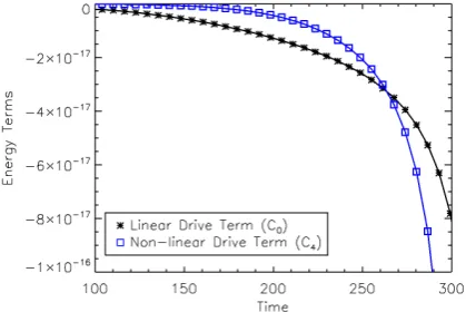
whereR dV =Rdx0dy0Lzis a volume integral. The dominant terms originated from the inertiaC0and from the explosive nonlinear termC4of Eq. (6). A standard estimate for the onset of the nonlinear regime is the time when the energy of the quadratic nonlinear drive term exceeds the energy of the linear drive term. From Fig. 3 we can evaluate this time to bet≈260.

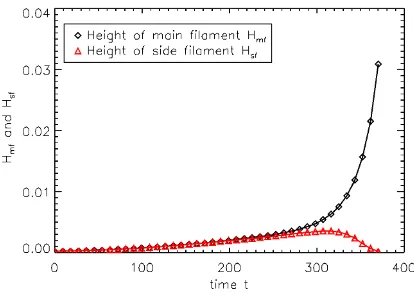
Through comparing the results of the simulations of the filaments of case 1 and case 3 we find that the main filament grows faster than in the single filament case. To explore this further, we investigate the height of the main filament with respect to the “ground level” because this ground level is always reduced in the nonlinear regime in the scope of this model [17]. The reasons for this is presented later. Thus we defineHmf(t) =ξ(x0= xmax, y= 0.0, t)−min(ξ(xmax, y, t)), see Fig. 4. The height of the side filament is defined in an equivalent manner. Evaluating the evolution of the two heights (see Fig. 5) one can clearly determine the linear and nonlinear phases and the time of the transition of the two which is consistent with the energy consideration. In the linear phase the side and main filaments grow equally. However, when the main filament enters the nonlinear regime the evolution starts to diverge such that the main filament grows stronger and eventually the side filament slows down and diminishes in size until it is fully suppressed. Comparing not only one flux surface but an entire set (Fig. 6) one can discover that the side filaments evolve towards different values ofx0away from the most unstable flux surface denoted byxmax.

To evaluate the solution of the combined modes with the sum of the two individual mode solution, case 2 and 3, we define

∆ξ=ξn1+n2−(ξn1+ξn2). (20)

Hereξn1+n2is the displacement of case 1 andξn1andξn2 are the solutions from case 2 and case 3, respectively.

We are expecting∆ξto be nearly zero at the beginning of the evolution when the linear terms dominate as the modes evolve independently since they satisfy the superposition principle: F(P_ixi) = PiF(xi), whereF

Fig. 3 Energies of the linearC0 (black,∗-symbols) drive term and the quadratic nonlinearC4 (blue,

represents the solution of the differential equation andxiare different initializations. As the plasma enters the nonlinear regime the superposition of the modes will deviate from the sum of the two distinct solutions. We are interested in how the interaction between the two modes changes their evolution. To explore this we examine∆ξ, as shown in Fig. 7. Positive values of∆ξimply that the coupled filaments grow further than the sum of the two individuals modes and negative values of∆ξmean that they grow slower. In Fig. 7 we show the spatial structure of∆ξdeep inside the nonlinear phase. The main filament is indicated by the positive∆ξpeak, and clearly grows stronger, suppressing the two side filaments for which∆ξ <0.

To normalize this change with respect to case 1, we define the interaction coefficientpi =

∆ξ ξn1+n2

for the main

filament, which characterizes the fraction of the main filament height due to the coupling to the side filaments. In the linear phasepiis also approximately zero, as expected, however, deep in the nonlinear regime, att= 370, the height of the main filament is over 80 % due to the interaction with the side filaments.

The mathematical origin of this behavior can be comprehended by analyzing the nonlinear ballooning equation. The dominant terms which determine the evolution in the nonlinear regime are the quasilinear nonlinearity term and the nonlinear growth drive therm. Both terms are composed of a contribution ofξ2_{which is an average ofξ}2

Fig. 4 The main filament height Hmf and the side filament heightHsf on the most unstable flux line is plotted. Note how the ”ground level” is reduced compared to zero – the equilibrium location of this flux surface.

Fig. 5 The temporal evolution atx0 = xmax of the main filamentHmf (black,♦-symbol) and the side filamentHsf(red,△-symbol) [10]

a) b)

Fig. 6 The flux surfaces in thex-yplane atz=L/2(half way between the plates). The color visualizes the displacement. The top is at the beginning of the nonlinear regimet≈260. The bottom shows the end of the simulation att= 370, which is deep in the nonlinear regime, just as the perturbed flux surfaces of case 1 are about to overtake each other:a)Initialized with three equal sized filaments (case 4). b)Central, main filament is initialized slightly larger (less than2%) than the two side filaments (case 1). At the later time the two side filaments are much smaller than the main central filament and the amplitude of the main filament is approximately 5 times larger than in case 4.

with respect of they0direction. Once one filament enters the nonlinear regime it grows explosively and domi-natesξ2_{. At this location the nonlinear growth drive termC4ξ}2_−ξ2_{will be positive asξ}2_{> ξ}2_{. Everywhere}

elseξ2 _{< ξ}2_{which causes the side filaments to be suppressed and the ground level to be reduced. The second}

nonlinearC3term consists ofC3ξ∂ 2_ξ2

∂x2 0

where the second derivative is pictured in Fig. 8. It is negative at the

most unstable flux surface and therefore serves as a damping term. However, further away from the most unstable location∂

2

ξ2

∂x2

0 reverses its sign and leads to a drive in the positivex0direction. This explains the remnants of the

side filaments further away from the most unstable flux surface, Fig. 6.

the plasma on top. Due to the incompressibility this plasma instead flows down on both sides of the main filament causing a down-draft which suppresses the side filaments.

2.5 Experimental observation

There exists experimental observations which may be described by our simulations presented here. We present two selected examples: type V ELMs in the NSTX tokamak [21] and ELMs in KSTAR [22]. The small, type V ELMs in NSTX involve fine-scale filaments that one would typically associate with higher toroidal mode number n. However, these ELMs only consist of one or two filaments which is in disagreement with what one would expect,∼nfilaments, from linear theory. While experimental evidence indicates the dominant instability drive is current density rather than ballooning modes, it is possible that a similar mechanism to that identified here acts to limit the number of filaments.

Another example which might be described by the nonlinear ballooning mode with interacting filaments are ELMs in KSTAR [22]. They observe slowly growing “fingers” out of the plasma which at some point sud-denly transforms into a more irregular formation followed by apparent suppression of filaments, which could be explained by the results presented here.

3

Type I ELMs in a MAST equilibrium

In this section a MAST Type I ELMy H-mode equilibrium is investigated (shot 24763). The fits of the profiles were produced by the standard equilibrium reconstruction code EFIT [23] and the equilibrium was calculated with the fixed boundary equilibrium solver HELENA which solves the Grad-Shafranov equation [24, 25].

Fig. 7 The spatial structure of∆ξdeep in the nonlinear regime. Note the holes at the position of the side filaments which indicate that they get “eaten” by the main-filament.

a) b)

Fig. 8 a)Sketch ofξ2 _{profile versusx}

0 which has a similar shape to a Gaussian. b)Sketch of ∂

2

ξ2

∂ψ2 profile which is of a

similar form of the second derivative of a Gaussian.

3.1 Nonlinear ballooning model for Tokamak geometries

To account for the tokamak geometry the Clebsch coordinate system is utilized where the magnetic field is written as [26]:

B0=∇ψ× ∇α (21)

whereαlabels the magnetic field lines on a certain flux surfaceψandαis chosen to be:

α=q(ψ)θ−φ (22)

whereφis the toroidal angle,θis the poloidal angle in straight field line coordinates andqis the safety factor which describes how many times a certain magnetic field line goes around the torus for one poloidal revolution. So far we have only chosen two variables for the Clebsch coordinate:ψandα. The third one can be chosen freely. Here we choose it as a poloidal angleχwhich increases by2πeach time a field line goes around poloidally. We generate new basis vectors: e⊥, e∧ and B₀ to decompose the quantities into perpendicular and parallel

components relative to the magnetic field line. The first two vectors are defined as:

e⊥≡∇

α×B0

B0 (23)

e∧≡

B0× ∇ψ

B0 (24)

e⊥ande∧are vectors perpendicular to the equilibrium magnetic field linesB0. The leading order displacement

can be again separated in the following way:

ξ(2) =ξ(ψ, α;t)

X

B0e⊥+GB0

=ξ(ψ, α;t)H (25)

whereHis defined as:H≡ X

B0e⊥+GB0. The ratio

X

B0 is independent of a fast variation ofψ,αandtand is

determined by the linear ballooning equation [19]:

(B0·∇0)

|e⊥|2

B2 0

(B0·∇0)X

+ 2µ

B4 0

(e⊥·κ0) (e⊥·∇0p0)X = 0 (26)

whereµis the so called ballooning eigenvalue. The equation describing the parallel component ofξ(2)is:

G=− 1 µ p′

0 |e⊥|2

B2 0

(B0·∇0)X (27)

The functionξwhich includes the perpendicular description of the leading order displacement is given by the nonlinear ballooning mode envelope equation for tokamak geometries [7, 16]:

C0 ∂ ∂α

∂2_ξ ∂t2 +C5

∂ ∂α ∂2 ∂t2 Z t 0

dt′ ξ(t ′

) (t−t′₎λ−1

=C1

2 (1−µ) ∂

∂αξ− ∂2_µ ∂f′2

∂2_u ∂ψ2

(28)

+C2 ∂ ∂αξ

2_+C3

"_∂ξ ∂ψ 2 − ∂ 2_u ∂ψ2 ∂ ∂αξ−

1 2

∂2_ξ2 ∂ψ2

#

+C4∂ξ ∂α

∂2_ξ2

∂ψ2 (29)

whereξ= ∂u_∂α, the flux functionf(ψ)can be related to the toroidal fieldBφand the major radiusR:f =BφR. λis defined asλ≡√1−4DM whereDM is the Mercier coefficient [27]. The coefficients include most of the information of the equilibrium geometry since they are mainly field-line averaged equilibrium quantities. We will investigate theC2coefficient in more detail, therefore its expression is provided as a representative example for the coefficients:

C2= *

XPb B0

+

where the bracketsh· · ·idenote integrals along the field aligned variableχ;±pχare the limits of these integrals, and:

XPb

B0 =H[(e⊥· ∇)H]·(B· ∇) [(B· ∇)H]−1/2H(e⊥· ∇) [H·(B· ∇) [(B· ∇)H]] (31)

+ 1

2B0[(H· ∇)H]· ∇αe∧· L(He⊥) + 2(e⊥·κ0) Q−H

B2

with

Q−≡

1 2

H(B_{· ∇}) ((B_{· ∇})H)− |(B_{· ∇})H_|2 (32)

H_≡ X

B0e⊥+GB0 (33)

whereκ0is the magnetic field curvature andLis the linear operator which is defined acting on a perpendicular vectorW⊥(with onlye⊥ande∧components) as:

L(W⊥)≡B₀·∇₀[B₀·∇₀(W⊥)]−(∇₀κ₀)·W⊥+[B0(B0·∇0) + 2κ0]

2

B2 0

(κ0·W⊥)

(34)

The nonlinear drive coefficientC2 has slowly converging integrands as their leading orders are proportional to|χ|(2−_2λS)

, whereλS is between 1 and 2. To minimize the numerical calculations we divide the integrals into numerically evaluated regions and remaining integrals at largeχwhich can be evaluated analytically. The coefficientsC4andC5include functions described by differential equations which must therefore be evaluated. TheC0,C3andC5coefficients are only used under certain conditions. TheC0coefficient must be used ifλ≥2. Ifλ < 2we compute and useC5 instead. C3 must be determined only if the geometry of the plasma is not up-down symmetric, otherwise it is close to zero. Since we only evaluate up-down symmetric equilibria, this coefficient and its corresponding term are neglected.

3.2 MAST coefficient

Here we discuss the results of the coefficients of the original MAST Type I ELMy equilibrium and for which we find the following coefficients:

C1≈5.501 C4≈ −1.4 (35)

C5≈2.878 C2≈ −33474 (36)

µ≈0.74 λ≈1.252 (37)

We notice that both nonlinear coefficients are negative. The negative sign of the nonlinear drive coefficient de-scribes an inwards instead of an outwards explosive drive; but the remaining qualitative behavior of the filaments would be the same as shown in previous work [17, 28]. To show this let’s start with the nonlinear ballooning equation implemented in the code Deton81(which is used to solve the nonlinear ballooning equation):

D0κ∂ λ

∂tλξ=

D1−(ψ−ψ0) 2

∆2

ξ−D2∂ 2_u

∂ψ2 +D3

ξ2−ξ2_+D4ξ∂ 2_ξ2

∂ψ2 (38)

If we transform:α→aα,t→τ t,ψ→pψandξ→xξwith

a= D1

D2

r

D4

D2 τ=

κ

r

D0κ

D1 (39)

p=

√ D1D4

D3 x=

D1

D3 (40)

1_{The nonlinear coefficients of Deton8 are related to the nonlinear coefficients of the nonlinear envelope equation as follows:D}

3=C2

andD4=C4. To obtain the equation calculated in the code Deton8, we are using the Taylor-expansion of the quantityµand calculating its

values numerically. We can setC3 = 0since we only analyze up-down-symmetric cases. Furthermore we integrate with respect toαand

exploit thatξ= 0_.

a) c)

b) d)

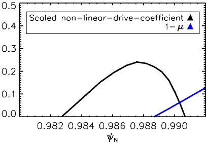
Fig. 9 Left: Profiles of the coefficients with the original equilibrium. a)The original ballooning eigenvalueµ. If this value is below1the plasma is ballooning unstable. b)The original explosive nonlinear drive coefficientC2. It continues to be

negative. Right: Profiles of the coefficients with an altered equilibrium where the local pressure gradient is increased by60%. c)The altered ballooning eigenvalueµ. If this value is below1the plasma is ballooning unstable.d)The altered explosive nonlinear drive coefficientC2. It now has a small but positive value nearψN= 0.987.

and

∆→√xp∆ (41)

we obtain a generic equation where∆is the only parameter. This generic equation was used previously [17, 28] and with it the qualitative results of filaments are similar. IfD3reverses its sign, the filaments move in the oppo-site direction, which can be seen by replacingξ→ −ξ. The only term that changes sign by this transformation is the nonlinear drive term. When the sign of the nonlinear drive coefficient is negative, the filament implodes rather than explodes.

However, if the quasilinear nonlinearity coefficient is also negative this leads to an imaginary transformation in the generic equation. This means that the change of this sign leads to a new generic equation. An in-depth dis-cussion of the effect can be found in [16]. Here we concentrate on the nonlinear drive coefficient as it determines the direction of the filament’s evolution. Next we investigate if we can find a positive nonlinear drive coefficient to compare this model with ELMs as we know that these have an explosive nature.

3.3 Coefficient profiles

The nonlinear ballooning model is valid if the ballooning eigenvalueµ is close to but smaller than 1 and if ∂µ

∂ψ ≈0.µ <1indicates that the plasma is ballooning unstable. ∂µ

∂ψ ≈0means thatµmust be a minimum [16]. This means that the values calculated for the coefficients are less precise further away from the extreme of the ballooning eigenvalue.

The ballooning eigenvalue has a broad minimum and differs by around20%from1, Fig. 9. Additionally we detect that the nonlinear drive coefficient continues to be negative on all flux-surfaces, but has a local maximum where the plasma is ballooning unstable.

The profiles obtained by increasing the local pressure gradient no longer represent an equilibrium, but help to un-derstand the dependencies of the coefficients. The nonlinear drive coefficient changes if the pressure gradient is adjusted, as illustrated in Fig. 9. Specifically, as the pressure gradient is increased the nonlinear drive coefficient is also increased. Additionallyλexceeds2which means that the normal inertial coefficient can be used [7]. Note that for this case there are flux surfaces which are ballooning unstable and have a positive nonlinear bal-looning drive, see Fig. 10. However, the local pressure gradient must be changed by60%in this case. This is larger than we would expect from experimental errors of the pressure gradient measurements which are around

20%[29].

3.4 Methods for experimental comparison

We must first identify an appropriate method to compare our results with experimental measurements . The most obvious one is to visualize the results of the simulations and compare these structures with observed structures in experiments. Here we present a method for direct comparison with MAST high speed camera measurements. This method is insufficient for quantitative comparison, therefore a heuristic energy model is presented next. It is used to calculate the energy released in an ELM from the simulated plasma. This energy can be easily compared with energies released in experiments.

We use the coefficients obtained from the case of the increased local pressure gradient, as it is a case which is ballooning unstable with a positive nonlinear drive. However the reader should keep in mind that the equilibrium pressure gradient is increased by60%which makes the comparison to experiments qualitative, at best. Neverthe-less these methods are presented to show that comparison between simulations and experiments is in principle possible.

3.4.1 3D visualization of filamentary structures

To display the perpendicular displacement of the filaments in Cartesian coordinates we first superimpose the so-lutions of the separated function_BX₀ andξˆgiven in equation (25), which are the solutions of the linear ballooning equation (26) and the nonlinear ballooning equation (29). Theψmeshes vary between the two codes (evaluating

Fig. 10 Scaled nonlinear drive coefficient and1₋µvs normalized flux surfaces. The plasma is ballooning unstable which means that the linear drive term is initially driving the filaments. Also the nonlinear drive coefficient is positive, which means that it drives the filaments outwards.

the linear and nonlinear ballooning equations), but we only display the displacement from the most unstable flux surface. The next step is to switch from the Clebsch coordinate system to a Cartesian system. We know that the cylindrical coordinateφis related to the Clebsch coordinateαby the following equation:

α=q(χ−χ0) +Y −φ (42)

whereχ0is a constant and the periodic functionY is defined as:

Y ≡

Z χ

0

νdχ−q(χ−χ0) (43)

withνdefined asν= f J

R2 and related to the safety factor:q=

1 2π

H

νdχ(see [19]).

With this relation we calculate the toroidal angleφfor each givenαandχ. Furthermore we know theZandR values for each givenχas these values are given in the input files for the coefficient code (in the MAST case produced by HELENA). We then exploit the transformation relations for cylindrical coordinates to Cartesian coordinates. A typical result of visualizing the filaments in 3 dimensions with an adjusted mode number2is shown in Fig. 11 where the data are depicted on top of a high speed camera image of an H-mode plasma in MAST. The brighter parts are regions with higher values of the displacement. Using this method, we could in principle compare simulations with fast camera observations, as long as the equilibrium used provided suitable coefficients for the nonlinear ballooning mode envelope equation.

3.4.2 Heuristic energy model

This model was continued from work presented in Reference [30, 31]. We know that the linear drive in toka-maks is caused by the pressure gradient. The linear drive in our nonlinear ballooning envelope equation (29) is proportional to the ballooning eigenvalue, described by the following relation:

1−µ= p

′ −p′

c

p′ (44)

wherep′

is the pressure gradient in the plasma andp′

cis the critical pressure gradient for instability [32]. In our heuristic energy model we use observations from experiments: first, that the region of the steep pressure gradient

Fig. 11 3D structure of the simulated fila-mentary displacement.

Fig. 12 Evolution of the normalized width ∆

∆_max of the pedestal (top

figure), the evolution of the normalized pressure gradient where the drop of it is seen (middle figure), and the evolution of the displacement (bot-tom figure). Note, that it is the very beginning of the nonlinear regime where the crash of the pressure gradient is initialized.

2_{The original mode number is reduced by a factor of approximately 20. This high mode number compared to experiments is probably}

(called pedestal) is increasing before an ELM crash and second that the pressure gradient collapses during an ELM crash [32]. Therefore we introduce a pedestal width that grows linearly with time in our model. This is linearly destabilizing, so the perturbation increases until the nonlinear terms are of the same order as the linear terms. Then we make the pressure gradient crash until the instantaneous force on the filaments is approximately zero, see Fig. 12.

To implement this model we must translate it into the correct form to input into our codes. The1−µis replaced by the Taylor expansion: 1−µ(ψ(0))− ∂ψ∂2µ2(ψ−ψ0)

2

= D1− (ψ−ψ0) 2

∆2 , which allows us to represent the

width of the pedestal by∆. To estimate the energy released during the drop in the pressure gradient we make the approximation that the released energy is proportional to the drop in pressure gradient, and the volume of the pedestal. With that we obtain from this heuristic model the energy released in one ELM cycle of∼0.65kJ. Typical energy released during one Type I ELM cycle in MAST are between0.5-1.7kJ [12, 33].

At this point these values are not predictive. One has to compare several of the calculated energies with experi-ments since we can adjust several quantities in the model. However it is already promising that it is possible to reach sensible values for the energy released, especially if we consider that there is no kink-drive in our model. This could explain why we had to increase the pressure gradient to find appropriate coefficients. A purely pres-sure driven ELM is typically a Type II ELM [3, 29] which exists in high collisionality regimes with reduced bootstrap current. Type II ELMs typically release less energy during one ELM cycle, which could explain why the obtained energy is at the lower range of the energies released in MAST.

To evaluate if the missing kink-drive is the explanation for the negative coefficients, the coefficients of a Type II ELM on JET have also be evaluated, but the nonlinear coefficients were also found to be negative [16].

4

Conclusion

If not controlled, ELMs are predicted to be a major challenge due to the potential detrimental effects on the plasma facing components in future tokamak devices. Therefore improving the understanding of this type of instability would enhance the feasibility of fusion energy produced by magnetically confined plasmas in tokamaks. We have presented a promising candidate, the nonlinear ballooning model, to describe ELMs quantitatively since several of its qualitative characteristics of explosive filaments are in agreement with experimental observations of ELMs.

Here we have presented results exploiting this model to investigate first whether the nonlinear interaction of explosive multiple filaments influence their evolution and second whether the nonlinear ballooning model can describe Type I and II ELMs quantitatively. The latter topic is of special interest because the model, once derived, is numerically inexpensive to analyze because one only has to solve two differential equations and therefore could be used for large scans.

In the Sect. 2, we have demonstrated how the interaction between plasma filaments of marginally altered initial amplitudes affects their later evolution by exploiting the nonlinear ballooning mode envelope equation. We showed that the more developed filament grows faster while suppressing the smaller filaments. It is expected therefore, that the filaments which first enter the nonlinear regime will dominate the physics of plasma eruptions. Despite the fact that our results are derived from a slab plasma model, the equation describing the evolution has the same features as in more complex magnetic geometries, including tokamaks [5, 7]. We therefore reason that the phenomenon of large filaments feeding off the smaller ones is a generic feature of ideal MHD. Supporting our model we presented two examples of experimental observations (Type V ELMs in NSTX and ELMs in KSTAR) which show dominant filaments in tokamak geometry where one would expect a higher mode number from linear theory.

This theory is only valid in the early nonlinear stages of the filamentary evolution, and it requires that the dominant filaments will have time to have formed before the model becomes invalid. It is therefore sensible to test these ideas in full, large scale simulations, close to marginal stability.

Recently, it has been shown that there exists equilibrium states with displaced filaments [34]. It remains to be understood how the explosive eruptions evolve to this new saturated state.

In the second part (Sect. 3), we presented that we obtained imploding filaments caused by a negative explosive drive term, but by changing the equilibria we were able to invert the sign. Therefore the results for the ELM equilibria indicate that either the nonlinear ballooning model is not sufficient to describe the explosive nature of

the filaments or that the coefficients themselves are too sensitive to the equilibria, since we can show that they can switch signs depending on the input parameters. Either way the current results suggest that the nonlinear ballooning model alone is insufficient to describe Type I or Type II ELMs quantitatively.

5

Acknowledgments

Part of this work is funded by the German National Academic Foundation (Studienstiftung des deutschen Volkes), the German Academic Exchange Service (DAAD - Stipendium f¨ur Doktoranden)

I would also like to mention that this work has been carried out within the framework of the EUROfusion Con-sortium and has received funding from the Euratom research and training programme 2014-2018 under grant agreement No 633053 and from the RCUK Energy Programme (grant number EP/I501045). The views and opinions expressed herein do not necessarily reflect those of the European Commission.

References

[1] J. Connor, R. Hastie, H. Wilson, and R. Miller, Phys. Plasmas5, 2687 (1998). [2] J. Connor, Plasma physics and controlled fusion40(2), 191 (1998).

[3] P. Snyder, H. Wilson, J. Ferron, L. Lao, A. Leonard, D. Mossessian, M. Murakami, T. Osborne, A. Turnbull, and X. Xu, Nuclear fusion44(2), 320 (2004).

[4] H. Wilson, Fusion Science and Technology61(2T), 122–130 (2012).

[5] O. Hurricane, B. Fong, and S. Cowley, Physics of Plasmas4(10), 3565–3580 (1997). [6] S. Cowley, H. Wilson, O. Hurricane, and B. Fong, Control. Fusions45, A31 (2003). [7] H. R. Wilson and S. C. Cowley, Physical Review Letters92(17), 175006 (2004). [8] S. Cowley, B. Cowley, S. Henneberg, and H. Wilson471(2180), 20140913 (2015).

[9] S. C. Cowley, B. Cowley, S. A. Henneberg, and H. R. Wilson, arXiv:1411.7797v1 [physics.plasm-ph] (submitted to Proc. Roy. Soc. A).

[10] S. Henneberg, S. Cowley, and H. Wilson, Plasma Physics and Controlled Fusion57(12), 125010 (2015).

[11] A. Kirk, T. Eich, A. Herrmann, H. Muller, L. Horton, G. Counsell, M. Price, V. Rohde, V. Bobkov, B. Kurzan et al., Plasma physics and controlled fusion47(7), 995 (2005).

[12] A. Kirk, H. Wilson, R. Akers, N. Conway, G. Counsell, S. Cowley, J. Dowling, B. Dudson, A. Field, F. Lott et al., Plasma physics and controlled fusion47(2), 315 (2005).

[13] A. Kirk, B. Koch, R. Scannell, H. Wilson, G. Counsell, J. Dowling, A. Herrmann, R. Martin, M. Walsh et al., Phys. Rev. Lett.96(18), 185001 (2006).

[14] A. Kirk, H. R. Wilson, G. F. Counsell, R. Akers, E. Arends, S. C. Cowley, J. Dowling, B. Lloyd, M. Price, and M. Walsh, Phys. Rev. Lett.92(Jun), 245002 (2004).

[15] H. Wilson, J. Connor, S. Cowley, C. Gimblett, R. Hastie, P. Helander, A. Kirk, S. Saarelma, and P. Snyder, paper TH/4-1Rb (2006).

[16] S. I. A. Henneberg, Filamentary plasma eruptions in tokamaks, PhD thesis, University of York, 2016. [17] S. C. Cowley and M. Artun, Physics Reports283, 185–211 (1997).

[18] L. D. Landau and E. Lifshitz, Fluid Mechanics, 2nd ed. edition (Elsevier Ldt, 2010). [19] J. W. Connor, R. J. Hastie, and J. B. Taylor, Proc. Roy. Soc.A(365), 1 (1979).

[20] I. Bronstein, K. Semendjajew, G. Musiol, and H. M¨uhlig, Verlag Harri Deutsch1(2008).

[21] R. Maingi, M. Bell, E. Fredrickson, K. Lee, R. Maqueda, P. Snyder, K. Tritz, S. Zweben, R. Bell, T. M. Biewer et al., Physics of Plasmas (1994-present)13(9), 092510 (2006).

[22] G. Yun, W. Lee, M. Choi, J. Lee, H. Park, C. Domier, N. Luhmann Jr, B. Tobias, A. Donn´e, J. Lee et al., Physics of Plasmas (1994-present)19(5), 056114 (2012).

[23] L. Lao, H. S. John, R. Stambaugh, A. Kellman, and W. Pfeiffer, Nuclear Fusion25(11), 1611 (1985).

[24] G. Huysmans, J. Goedbloed, and W. Kerner, Proc. Europhysics 2nd Intern. Conf. on Compputational Physics, 10-14 Sept. 1990 pp. 371–376 (1991).

[25] C. Konz and R. Zille, HELENA - Fixed boundary equilibrium solver, Max-Planck-Institut f¨ur Plasmaphysik, Garch-ing, October 2007.

[26] W. D. D’haeseleer, W. N. Hitchon, J. D. Callen, and J. L. Shohet, Flux coordinates and magnetic field structure: a guide to a fundamental tool of plasma theory (Springer Science & Business Media, 2012).

[27] C. Mercier, Nuclear Fusion1(1), 47 (1960).

[28] B. H. Fong, S. C. Cowley, and O. A. Hurricane, Physical Review Letters82(23), 4651–4654 (1999).

[29] S. Saarelma, A. Alfier, M. Beurskens, R. Coelho, H. Koslowski, Y. Liang, I. Nunes et al., Plasma physics and controlled fusion51(3), 035001 (2009).

[31] S. A. Henneberg, S. C. Cowley, and H. R. Wilson, European Physical Society, Germany, (2014).

[32] D. Dickinson, S. Saarelma, R. Scannell, A. Kirk, C. Roach, and H. Wilson, Plasma physics and controlled fusion 53(11), 115010 (2011).

[33] A. Kirk, G. F. Counsell, G. Cunningham, J. Dowling, M. Dunstan, H. Meyer, M. Price, S. Saarelma, R. Scannell, M. Walsh, H. R. Wilson, and the MAST team, Plasma Physics and Controlled Fusion49(8), 1259 (2007).

[34] C. J. Ham, S. C. Cowley, G. Brochard, and H. R. Wilson, Phys. Rev. Lett.116(Jun), 235001 (2016).