Fault-Tolerant Quantum Computing
.
White Rose Research Online URL for this paper:
http://eprints.whiterose.ac.uk/113586/
Version: Accepted Version
Article:
Campbell, E. and Howard, M. (2017) Application of a Resource Theory for Magic States to
Fault-Tolerant Quantum Computing. Physical Review Letters, 118. 090501. ISSN
0031-9007
https://doi.org/10.1103/PhysRevLett.118.090501
[email protected] https://eprints.whiterose.ac.uk/ Reuse
Unless indicated otherwise, fulltext items are protected by copyright with all rights reserved. The copyright exception in section 29 of the Copyright, Designs and Patents Act 1988 allows the making of a single copy solely for the purpose of non-commercial research or private study within the limits of fair dealing. The publisher or other rights-holder may allow further reproduction and re-use of this version - refer to the White Rose Research Online record for this item. Where records identify the publisher as the copyright holder, users can verify any specific terms of use on the publisher’s website.
Takedown
If you consider content in White Rose Research Online to be in breach of UK law, please notify us by
Application of a resource theory for magic states to fault-tolerant quantum computing
Mark Howard∗ and Earl Campbell†
Department of Physics and Astronomy, University of Sheffield, Sheffield, UK
Motivated by their necessity for most fault-tolerant quantum computation schemes, we formulate a resource theory for magic states. We first show that robustness of magic is a well-behaved magic monotone that operationally quantifies the classical simulation overhead for a Gottesman-Knill type scheme using ancillary magic states. Our framework subsequently finds immediate application in the task of synthesizing non-Clifford gates using magic states. When magic states are interspersed with Clifford gates, Pauli measurements and stabilizer ancillas—the most general synthesis scenario— then the class of synthesizable unitaries is hard to characterize. Our techniques can place non-trivial lower bounds on the number of magic states required for implementing a given target unitary. Guided by these results we have found new and optimal examples of such synthesis.
Quantum resource theories attempt to capture what is quintessentially quantum in a piece of technology. For example, entanglement is the relevant resource for quan-tum cryptography and communication. The resource framework for entanglement finds practical application in bounding the efficiency of entanglement distillation pro-tocols. An abundance of other resource theories have been related to various aspects of quantum theory [1– 8]. Once a quantum computer is made fault-tolerant, some computational operations become relatively easy, and some more difficult, leading to a natural resource picture called the magic state model [9,10] (although al-ternative routes to fault-tolerant universality exist [11]). Preparation of stabilizer states and implementation of Clifford unitaries and Pauli measurements constitute free resources. Difficult operations include preparation of magic states, a supply of which is necessary in order to promote the easier operations to a universal gate set. With only free resources, the computation can be effi-ciently classically simulated, whereas with a liberal sup-ply of pure magic states, universal quantum computation is unlocked. For qudit (d-level) quantum computers with oddd, a resource theory of magic (or equivalently contex-tuality with respect to stabilizer measurements [12, 13]) has been developed [7, 14, 15]. This relies on a well-behaved discrete Wigner function [16], which in turn re-lies on quirks of odd dimensional Hilbert space. Here we address the most practically important case by quan-tifying the magic for multiqubit systems, relating this resource measure to simulation complexity and applying the resource theory to the practical problem of gate syn-thesis.
The canonical magic state is|Hi= (|0i+eiπ/4|1i)/√2, which enables application of a single-qubit unitary T = diag(1, eiπ/4) [9, 10]. A circuit composed of elements from the Clifford+T gate set acting on the standard computational basis input suffices for universal quantum computation. Such a circuit can be classically simulated, but in a time that scales exponentially in the number of T gates [17]. Faster simulation algorithms were re-cently discovered that relate the simulation complexity to the stabilizer rank [18–20], a measure of magic for pure
states. Such techniques do not naturally adapt to mixed magic states, and stabilizer rank is qualitatively very dif-ferent to the magic measure we establish here. For quan-tum computations using qudits with odd dimension, the discrete Wigner function provides a quasiprobabilitiy dis-tribution and Pashayan et al. [21] showed that the nega-tivity quantifies the simulation complexity. Here we pro-vide a general simulation scheme, which can be naturally applied to mixed-state qubit quantum computations us-ing any kind of ancillary magic state (e.g., a multi-qubit magic state enabling a Toffoli gate). Furthermore, for many problems our approach is competitive with compa-rable schemes based on stabilizer rank [18,19].
The Supplementary Materials (text, which includes Refs. [32–36], and files) contain numerous additional computations. Results include identifying the most ro-bust states, most roro-bust gates and classification of all three and four qubit diagonal gates from the third level of the Clifford hierarchy. Intriguingly, one maximally ro-bust state is the Hoggar [37] fiducial state.
Robustness of Magic.—Vidal and Tarrach [8] showed that the amount of separable noise that makes an entangled state become separable is an entanglement monotone, which they called robustness. The basic principle can been adapted for use in other resource theories with a set of free states. DenotingSn ={σi} as the set of pure n-qubit stabilizer states, we define the robustness of magic as
(RoM) R(ρ) = min x
( X
i
|xi|;ρ= X
i xiσi
) . (1)
Decompositions of the formP
ixiσi are called stabilizer pseudomixtures. We haveP
ixi= 1, butxi may be neg-ative and so they provide a quasiprobability distribution. The optimization in (1) can be rewritten in terms of a linear system as
R(ρ) = min||x||1 subject toAx=b , (2)
where||x||1=Pi|xi|,bi= Tr(Piρ) andAj,i= Tr(Pjσi) wherePjis thejth Pauli operator. For example, consider the single-qubit magic state |Hi = (|0i+eiπ/4|1i)/√2, then in the Pauli operator basis
A= h11i hXi hYi hZi
1 1 1 1 1 1 1 −1 0 0 0 0 0 0 1 −1 0 0 0 0 0 0 1 −1
, b=
1 1
√
2 1
√
2 0
,
and the solution of (2) is x= √2,0,1,1−√2,0,0 /2 implying R(|Hi) = √2. There are a number of freely available solvers for linear programs [38,39], which are ef-ficient in the size ofA. From our formulation of the prob-lem it is clear that minAx=b||x||1is feasible and bounded. Consequently, strong duality holds i.e.,
min
Ax=b||x||1=||ATmax
y||∞≤1
−bTy , (3)
and the aforementioned solvers can provide a certificate y of optimality [40]. Despite the theoretical efficiency of the linear programming problem, the number of stabi-lizer states in Pn scales super-exponentially with n, so that|Sn|= 2nQnj=1(2j+ 1) [16]. Practically we are lim-ited to 1 ≤n ≤5 qubits. We have made available the correspondingAmatrices in Supplementary Material.
Robustness of Magic (RoM) possesses all the desir-able qualities of a resource theoretic measure (see Sup-plementary Material for proofs of the following). For a
..
.. |U
|ψ
U|ψ
m1
mn Clifford Correction
|H
|H |H
S m2
S m1
Y S
m3
S =
T T
T† =
S
(a)
(b)
(c)
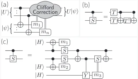
FIG. 1. (a) Half-teleportation gadget for implementing diag-onalU in the third level of the Clifford hierarchy. The circuit uses a resource state|Ui=U|+i⊗n. (b) Exact synthesis of CS gate usingT-gates and CNOTS. (c) The CS circuit as a gad-getized circuit using three|Himagic states. Our techniques show this synthesis is provably optimal.
mixed stabilizer state, we findxi>0 entailingPi|xi|= P
ixi = 1. For a non-stabilizer state, at least one xi is negative and then RoM must exceed unity. Therefore RoM is faithful. Crucially, RoM is non-increasing un-der stabilizer operations, the free set of operations in the resource theory. Finally, RoM is submultiplicative,
R(ρ1⊗ρ2)≤ R(ρ1)R(ρ2), (4)
which follows by using the minimal stabilizer pseudomix-tures forρ1andρ2to construct a not-necessarily-minimal stabilizer pseudomixture forρ1⊗ρ2. Useful lower bounds onR(ρ1⊗ρ2) can also be obtained (see Supplementary Material).
Resource theoretic frameworks are commonplace in quantum information theory, but do not always directly lend themselves to an operational meaningful interpre-tation or to useful applications in solving relevant prob-lems. In the next section we show how RoM quantifies the exponential simulation overhead for a version of the Gottesman-Knill protocol where non-stabilizer ancillasρ can be added to an otherwise stabilizer circuit. The sub-sequent section discusses RoM’s application to the task of implementing non-Clifford operations in an economical way.
Robustness quantifies classical simulation overhead.—
[image:3.612.321.557.54.190.2]3
an expectation value Pρ := tr[PE(ρ)] where E is a sta-bilizer operation. The simulation time cost scales with P
i|xi| ≥ R(ρ) wherexi are the quasiprobabilities used (which may be suboptimal). First, as in [21], we use the quasiprobability distribution xi to form the prob-ability distribution pi = |xi|/Pi|xi|. We sample an i value from this probability distribution and use GK to obtain an eigenvalue m = ±1 for the Pauli mea-surement on E(σi). Our simulation outputs not m, but M = sign(xi)mPi|xi|where sign(xi) = 1 forxi>0 and sign(xi) = −1 otherwise. Notice that each run outputs ±P
i|xi| and not ±1, which leads to a larger variance of our random variable. We repeat this sampling process many times and find the mean value ofM, which gives an unbiased estimator ofPρ. The Hoeffding inequalities show that for random variables bounded in the interval [−P
i|xi|,+ P
i|xi|], N samples will estimate the mean to within δ of the actual mean with probability exceed-ing 1−ǫ where ǫ = 2 exp(−N δ2/2(P
i|xi|)2). In other words, the desired accuracy is guaranteed by using
N = 2 δ2(
X i
|xi|)2ln 2
ǫ
(5)
samples. Using an optimal stabilizer pseudomixture, the number of samples scales quadratically in the robustness, though the robustness typically scales exponentially in the number of magic states. For each of these samples, the GK scheme requires a polynomial amount of time provided we know how to efficiently sample from the quasiprobabilitiy distribution.
Nonstabilizer circuits.—For any quantum circuit we can find an equivalent gadgetized version [9,18,19] over the Clifford plusT gate set; all uses of T are replaced with the standard state injection circuit whereby a|Histate is entangled with a data qubit and subsequently mea-sured out (see Fig. 1 for an example). The T gadget is just one example from an infinitely large family of simi-lar gadgets. All diagonal gates from the third level of the Clifford hierarchy—the set of gates that map Pauli oper-ators to Clifford gates under conjugation—are also suit-able for gadgetization. These gates are sufficient to pro-mote Clifford gates to universality, and have the added property that access to the state |Ui = U|+i⊗k allows for deterministic implementation of the gateU [44,45], as depicted in Fig. 1. This family includes important multiqubit gates such as the control-control-Z (CCZ), which is Clifford equivalent to the Toffoli, and control-S (Ccontrol-S) where S = T2. Therefore, a quantum circuit C1U1C2U2. . . UNCN+1 where Ci are Clifford is equiva-lent to a stabilizer circuit consuming the resource |Ui where U := ⊗Uj. We remark that diagonal, third-level gates are exactly synthesizable from CNOT and T gates [22, 23, 46,47].
Large resource states.— For large resource states the exact robustness may be difficult to determine. How-ever, instead of using the optimal robustness we instead
use stabilizer psuedomixtures built up from constant size blocks of qubits, here limited to 5 qubits per block. For instance, givent=bmcopies of the|Histate, we break it into b blocks of m-qubits (|Hi⊗m)⊗b and so work with a pseudomixture whose sample complexity scales asP
i|xi|=R(|Hi⊗m)b = h
R(|Hi⊗m)1 m
it .
Numerical results.— We performed substantial numeri-cal investigations up to 5 qubit systems, for which there are over two million stabilizer states and over one thou-sand Pauli operators. For ascendingm≤5 we calculated R(|H⊗mi)1
m as {1.414,1.322,1.304,1.301,1.298}. The
decrease withm shows a strongly submultiplicative be-haviour and reduces simulation overheads (though ana-lytic lower bounds derived in Supplementary Materials show going to higher m cannot reduce this value be-low 1.207). Specifically,R(|H⊗5i)2t
5 ≈1.2982t= 1.685t
characterises the complexity of our Clifford plust T gate simulation. This gives exponential improvement over the method used in [19] with complexity scaling as 1.9185t. A more efficient use of the stabilizer Schmidt decomposi-tion was subsequently established in [18], leading to com-plexity scaling as 1.385t, although the restriction to pure states as in [19] also holds here. Even better scaling with tcan be obtained by using approximate states [18], but at the price ofδ−5 overhead in the precisionδ. A quantum computation usingz CCZgates, can be implemented us-ing 4z T gates [31], implying our simulation complexity scales as 8.067z. However, as discussed earlier, we can use |CCZi resource states. We found R(|CCZi) = 2.555, and soz CCZs can be simulated with an overhead dom-inated byR(|CCZi)2z = 6.531z. This gives exponential improvement over using the four-T-gate gadgetization. Alternative gadgetizations using|Ui=U|+iwith third-level diagonalUfollow naturally and the simulation over-head is given byR(|Ui), see Supplementary Material for many possible examples.
Lower bounds on gate synthesis.—Beyond classical sim-ulation, robustness can help us investigate gate synthesis. Above, we noted that fourT gates can exactly synthesize a CCZ gate. How can we be sure that a more compli-cated or clever scheme does not use even fewerT gates, not just for CCZ gates but more generally? This is an important instance where our resource theory of magic applies; a potential resource state|Ui=U|+ifor a non-Clifford unitary U cannot be made using t T gates if R(|Ui)>R(|H⊗ti). The resource state|CCZi, Clifford-equivalent to a Toffoli resource, has R(|CCZi) = 2.555 implying
R(|H⊗3i)<R(|CCZi)<R(|H⊗4i). (6)
of optimality for many more unitaries.
Improved gate synthesis.— Circuit synthesis can be purely unitary over the Clifford+T gate set, or more generally can make use of stabilizer ancillas and mea-surement thereby using even fewerT gates. The scale of the potential savings is exemplified by the four T gate realisation of CCZ [31], which is assisted by ancillas and measurement. Purely unitary synthesis ofCCZover Clifford+T is known to need at least sevenT gates [24]. We shed new light on this phenomena by showing that it emerges from Clifford equivalence of magic states, and give new examples of improved synthesis. The interest-ing examples arise when C|Ui = |Vi, and yet unitary synthesis ofU uses fewerT-gates thanV. For these re-markable examples, despite Clifford equivalence of states |Uiand|Vi, there do not exist CliffordsC1andC2 such that C1U C2=V. One explicit example, comparable to Jones’ construction [31], starts with the Toff∗ gate cor-responding to CCZ123CS12, which is known to be uni-tarily synthesizable using fourT gates [29]. Because the “square-root-of-NOT”√Xis a Clifford gate, we also have that
II√X|Toff∗i=|CCZi. (7) Clifford equivalence of magic states provides an alterna-tive proof thatCCZcan be performed with fourT gates. We have found a number of similar examples using the following method (i) Identify U and V with differ-ent T-count but whose states have the same robustness R(|Ui) =R(|Vi), (ii) Search for the CliffordCthat takes |Uito|Vi. Existence of such a Clifford is not guaranteed by virtue ofR(|Ui) =R(|Vi), but we found a Clifford in every instance investigated. Note also that ourT count is over the CNOT+T basis, which is less general than the Clifford+T basis but existing techniques for the lat-ter [24] are impractical for more than three qubits. The two methods (Clifford+T and CNOT+T) give the same
T count for CCZ and it is an interesting open question whether they always agree on theT cost of synthesizing a third-level gate. We list, in compact notation, a few of the new synthesis results and theT savings (more are provided in Supplementary Material). For example the
CCZconstruction discussed above would be represented as
CCZ1237−→→4CS12CCZ123, (8)
where the subscripts denote the qubits on which a third-level gate acts and the numbers above the arrow denote theT cost. Other examples include
CCZ123−→7→4CS12CS13, (9)
CCZ123,14511−→→8CS12,13,14,15, (10)
T1,2,3CS12,23,13−→6→5T2,3CS12,23,13. (11)
Discussion.-By reformulating robustness as an optimiza-tion in (2) this facilitates a comparison with recent re-lated works see Table I. For qudit-based computation, Veitch et al. [7] showed that sum-negativity sn(ρ) of a state’s discrete Wigner function was a well-defined re-source and Pashayan et al. [21] showed how the run time of a Monte-Carlo type sampling algorithm was slower by a factor quadratic in the size of the sum-negativity. In the qudit setting the natural choice for the columns of Ain Eq. (2) are the vertices of the Wigner polytope (a larger, but more geometrically simple object than the stabilizer polytope), and phase point operators form a natural operator basis. With these choices, b is a vec-torised version of the Wigner representation ofρand the matrixA becomes the identity matrix. R(ρ) is simply the sum-negativity (equal to theℓ1 norm) of the Wigner quasiprobability distribution associated withρ. In other words, sum-negativity is just robustness relative to the set of operators with non-negative discrete Wigner func-tion. Unlike our approach, the discrete Wigner-function is not easily adapted to qubits (although see [48, 49]).
In work by Bravyi, Smith and Smolin [19]t-fold copies of |Hi are decomposed as linear combinations of stabi-lizer vectors [20]; the number of terms χ—the stabilizer Schmidt rank—in the decomposition quantifies the sim-ulation overhead. Finding the optimal decomposition is an ℓ0 minimization (||x||0 = |{i : xi 6= 0}|), which is non-convex and NP-hard, limiting calculations to small number of qubits. Bravyi and Gossett [18] extended this analysis by efficiently finding approximate decomposi-tions that are still sufficient for the task of simulating the outcome of a quantum algorithm. This approxima-tion precludes the possibility of ordering states by the amount of resource, however. We note that it is well known in the signal processing literature [50] that the so-lution toℓ1 minimization also provides a (qualitatively) good solution forℓ0minimization.
Resource |ψi ∈Cd ρ∈B(H)
χ(|ψi) =||x||0 BSS[19], BG[18]
sn(ρ) =||x||1 PWB[21], VMGE[7]
R(ρ) =||x||1 This Work
TABLE I. Restatement of related work in terms of norm-minimizing solutions of a system of equationsAx =b. The amount of resource in an ancillary state|ψiorρquantifies the classical simulation overhead. In the first and third lines the columns ofAaren-qubit stabilizer states (as complex vectors or generalized Bloch vectors, respectively). In the second line the columns ofAare extreme points of the Wigner polytope.
5
seen to disagree with almost every other continuous en-tanglement measure. A related open problem is to rec-oncile the fact that small angle ancillae (1, eiφ≈0)/√2 are cheap in our framework, yet are harder to synthesize over the Clifford+T gate [28] set and harder to fault-tolerantly distill [26, 52]. Considerations such as this suggest that a combination of both the stabilizer Schmidt rank and robustness pictures of magic could prove useful.
Acknowledgments The authors thank Naomi Nickerson for reviving our interest in this problem and acknowledge funding from Engineering and Physical Sciences Research Council (Grant No. EP/M024261/1).
∗ m.howard@sheffield.ac.uk † [email protected]
[1] F. Brand˜ao and G. Gour,Phys. Rev. Lett.115, 070503 (2015).
[2] B. Coecke, T. Fritz, and R. W. Spekkens,Information and Computation (2016), 10.1016/j.ic.2016.02.008. [3] A. Grudka, K. Horodecki, M. Horodecki, P. Horodecki,
R. Horodecki, P. Joshi, W. K lobus, and A. W´ojcik,Phys. Rev. Lett. 112, 120401 (2014).
[4] M. Horodecki and J. Oppenheim, Int. J. Mod. Phys. B
27, 1345019 (2013).
[5] C. Napoli, T. R. Bromley, M. Cianciaruso, M. Piani, N. Johnston, and G. Adesso, Phys. Rev. Lett. 116, 150502 (2016).
[6] D. Stahlke,Phys. Rev. A90, 022302 (2014).
[7] V. Veitch, S. A. H. Mousavian, D. Gottesman, and J. Emerson,New J. Phys.16, 013009 (2014).
[8] G. Vidal and R. Tarrach,Phys. Rev. A59, 141 (1999). [9] S. Bravyi and A. Kitaev,Phys. Rev. A71, 022316 (2005). [10] E. Knill,Nature434, 39 (2005).
[11] E. T. Campbell, B. M. Terhal, and C. Vuillot, arXiv:1612.07330 [quant-ph] (2016), arXiv:1612.07330 [quant-ph].
[12] M. Howard, J. Wallman, V. Veitch, and J. Emerson,
Nature510, 351 (2014).
[13] N. Delfosse, C. Okay, J. Bermejo-Vega, D. E. Browne, and R. Raussendorf, arXiv:1610.07093 [quant-ph] (2016),arXiv:1610.07093 [quant-ph].
[14] V. Veitch, C. Ferrie, D. Gross, and J. Emerson,New J. Phys.14, 113011 (2012).
[15] A. Mari and J. Eisert, Phys. Rev. Lett. 109, 230503 (2012).
[16] D. Gross, Journal of Mathematical Physics47, 122107 (2006).
[17] S. Aaronson and D. Gottesman,Phys. Rev. A70, 052328 (2004).
[18] S. Bravyi and D. Gosset, Phys. Rev. Lett.116, 250501 (2016).
[19] S. Bravyi, G. Smith, and J. A. Smolin,Phys. Rev. X6, 021043 (2016).
[20] H. J. Garc´ıa, I. L. Markov, and A. W. Cross, Quantum Information & Computation14, 683 (2014).
[21] H. Pashayan, J. J. Wallman, and S. D. Bartlett,Phys. Rev. Lett. 115, 070501 (2015).
[22] M. Amy, D. Maslov, and M. Mosca,IEEE Transactions on Computer-Aided Design of Integrated Circuits and
Systems33, 1476 (2014).
[23] M. Amy and M. Mosca, arXiv:1601.07363 [quant-ph] (2016),arXiv:1601.07363 [quant-ph].
[24] D. Gosset, V. Kliuchnikov, M. Mosca, and V. Russo, Quantum Information & Computation14, 1261 (2014). [25] A. Bocharov, Y. Gurevich, and K. M. Svore,Phys. Rev.
A88, 012313 (2013).
[26] G. Duclos-Cianci and K. M. Svore, Phys. Rev. A 88, 042325 (2013).
[27] A. Paetznick and K. M. Svore, Quantum Information & Computation14, 1277 (2014).
[28] N. J. Ross and P. Selinger, arXiv:1403.2975 [quant-ph] (2014),arXiv:1403.2975 [quant-ph].
[29] P. Selinger,Phys. Rev. A87, 042302 (2013).
[30] N. Wiebe and M. Roetteler, Quantum Information and Communication16, 134 (2016).
[31] C. Jones,Phys. Rev. A87, 022328 (2013).
[32] D. Andersson, I. Bengtsson, K. Blanchfield, and H. B. Dang,J. Phys. A48, 345301 (2015).
[33] B. W. Reichardt, Quantum Information & Computation 9, 1030 (2009).
[34] E. T. Campbell,Phys. Rev. A83, 032317 (2011). [35] A. W. Harrow and M. A. Nielsen, Phys. Rev. A 68,
012308 (2003).
[36] W. van Dam and M. Howard,Phys. Rev. A83, 032310 (2011).
[37] S. G. Hoggar,Geometriae Dedicata69, 287 (1998). [38] M. Grant and S. Boyd, inRecent Advances in Learning
and Control, Lecture Notes in Control and Information Sciences, edited by V. Blondel, S. Boyd, and H. Kimura (Springer-Verlag Limited, 2008) pp. 95–110.
[39] M. Grant and S. Boyd,CVX: Matlab Software for Disci-plined Convex Programming, Version 2.1 (2014). [40] This certificate of optimality can be used to obtain
a magic witness—an operator whose expectation value with respect to stabilizer states is in the interval [−1,1] and whose expectation with respect toρisR(ρ). These witnesses can be used to derive exact expressions for ro-bustness as in Supplementary Material.
[41] H. Buhrman, R. Cleve, M. Laurent, N. Linden, A. Schri-jver, and F. Unger, in 2006 47th Annual IEEE Sym-posium on Foundations of Computer Science (FOCS’06)
(2006) pp. 411–419.
[42] S. Virmani, S. F. Huelga, and M. B. Plenio, Physical Review A71, 042328 (2005).
[43] M. B. Plenio and S. Virmani,New Journal of Physics12, 033012 (2010).
[44] D. Gottesman and I. L. Chuang,Nature402, 390 (1999). [45] X. Zhou, D. W. Leung, and I. L. Chuang,Phys. Rev. A
62, 052316 (2000).
[46] E. T. Campbell and M. Howard, arXiv:1606.01904 [quant-ph] (2016),arXiv:1606.01904 [quant-ph]. [47] E. T. Campbell and M. Howard, arXiv:1606.01906
[quant-ph] (2016),arXiv:1606.01906 [quant-ph]. [48] N. Delfosse, P. Allard Guerin, J. Bian, and
R. Raussendorf,Phys. Rev. X5, 021003 (2015). [49] R. Raussendorf, D. E. Browne, N. Delfosse, C. Okay, and
J. Bermejo-Vega, arXiv:1511.08506 [quant-ph] (2015),
arXiv:1511.08506 [quant-ph].
[50] E. Candes and T. Tao,IEEE Transactions on Information Theory51, 4203 (2005).
[51] M. Van den Nest,Phys. Rev. Lett.110, 060504 (2013). [52] E. T. Campbell and J. O’Gorman,Quantum Science and
APPENDIX
Robustness of magic
Here we give a more extended discussion of the proper-ties of RoM and also introduce techniques for obtaining lower bounds. We first tackle the basic properties, which are standard for robustness measures of a resource and our proofs will parallel work elsewhere [8]. In contrast, our results on lower bounds (see Sec. ) are tailored to the magic state setting and do not have counterparts in other resource theories. Note that robustness is mostly described here in algebraic terms but a geometric picture as in Fig2 is natural.
·
ρ
ρ+
[image:7.612.110.245.240.335.2]ρ−
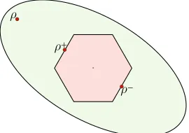
FIG. 2. Robustness of magic (geometric): The hexagon represents all possible mixtures of stabilizer states i.e., the stabilizer polytope. Highlighted points correspond to the state of interest, ρ, and two stabilizer states, ρ±, such that ρ= (p+ 1)ρ+−pρ−. Calculating robustness of magicR(ρ)
requires optimizing over all such decompositions but this may be recast as a linear program (Eq. (2) of main text). This is completely analagous to the original formulation of robust-ness of entanglement [8] except here the extreme points of the set of free states form a discrete set.
Basic properties
We list the basic properties of the robustness of magic
R1 Faithfulness:R(ρ) = 1 if and only ifρis a stabilizer state, and otherwise R(ρ)>1.
R2 Submultiplicativity: R(ρ1⊗ρ2)≤ R(ρ1)· R(ρ2);
R3 Monotonicity: for all trace-preserving stabilizer channels E, we haveR(E(ρ))≤ R(ρ).
R4 Convexity: R(P
kpkρk)≤ P
k|pk|R(ρk). Let us prove these properties one by one.
Faithfulness.-Ifρis a mixed-stabilizer state then by def-inition there exists a decomposition ρ =P
ipiσi where pi are positive and so settingxi =pi we havePi|xi|= P
ixi = 1. Conversely, if ρ is nonstabilizer state, then there is at least one negative value of xi. Furthermore, Tr(ρ) = 1 entailsP
ixi = 1 and so we can express the
absolute sum as P
i|xi| = 1 + 2 P
i:xi<0|xi| where the
new summation is only over the negative values. We see that if a single value is negative, then the RoM exceeds unity.
Submutliplicativity.- Let ρ1 and ρ2 have optimal pseu-domixtures
ρ1= X
i
xiσi, (12)
ρ2= X
j yjσj,
where optimality entails R(ρ1) = Pi|xi| and R(ρ2) = P
j|yj|. We consider the composite state
ρ1⊗ρ2= X
i,j
xiyj(σi⊗σj). (13)
Sinceσi⊗σjare pure stabilizer states, this is a stabilizer pseudomixture with quasiprobabilitiesxiyj. Taking the absolute sum we have
X i,j
|xiyj|= X
i |xi|
!
X j
|yj|
(14)
=R(ρ1)R(ρ2).
Therefore,R(ρ1⊗ρ2)≤ R(ρ1)R(ρ2).
Monotonicity.-IfE is stabilizer operation, thenE(σi) = P
jpi,jσj where pi,j ≥ 0. Furthermore, if E is trace-preserving then, for all i, we have P
jpi,j = 1. Com-bined with positivity we knowP
j|pi,j|= 1. Therefore, applyingE to an arbitrary state
E(ρ) =X i
xi X
j
pi,jσj, (15)
=X
j X
i xipi,j
! σj,
which is a stabilizer pseudomixture with quasiprobabili-tiesx′
j= P
ixipi,j. Therefore,
R(E(ρ))≤X j
|X i
xipi,j|. (16)
Using the triangle inequality |P
kak| ≤ Pk|ak| and |ab|=|a| · |b|, we have
R(E(ρ))≤X i
|xi| X
j
|pi,j| (17)
=X
i |xi|
=R(ρ).
7
e.g. postselection on a particular outcome of a stabilizer POVM. The proof proceeds along the same lines as that provided in [8].
Convexity.-Consider a set of quantum states with opti-mal stabilizer pseudomixtures
ρk= X
i
x(k)i σi, (18)
so thatR(ρk) =Pi|x (k)
i |. It follows that
X k
pkρk= X
i X
k
pkx(k)i σi. (19)
Takingx′
i= P
kpkx(k)i as quasiprobabilities we have
R X
k pkρk
!
≤X
i |X
k
pkx(k)i |. (20)
Applying the triangle inequality, we have
R X
k pkρk
!
≤X
i X
k
|pk| · |x(k)i | (21)
=X
k
|pk|R(ρk).
This proves convexity.
Taking the logarithm of the robustness creates a re-lated measure LR such that LR(ρ) = log2(R(ρ)). It immediately follows that LR is also monotonically de-creasing under stabilizer channels. Submultiplicativity translates into subadditivity. Furthermore, LR is faith-ful in the sense that LR(ρ) = 0 if and only if ρ is a stabilizer state.
Lower bounds on RoM
This section introduces a new quantity that we use to establish lower bounds on RoM. Such bounds are valu-able since numerical methods are limited to modest num-bers of qubits, whereas the lower bounds will hold for any number of qubits.
We define D (also called the st-norm || · · · ||st in Ref. [34]) as
D(ρ) = 1 2n
X P∈P+
|Tr(P ρ)|, (22)
where P+ is the set of Pauli operators with +1 phase, including the identity. It has some useful properties,
D1 Convexity: D(P
kpkρk)≤ P
k|pk|D(ρk) ,
D2 Magic witness: ifD(ρ)>1 thenρis a nonstabilizer state,
D3 Lower bound: D(ρ)≤ R(ρ),
D3* Tighter lower bound: Ifρis ann-qubit state then
D(ρ)−21n
1−21n
≤ R(ρ), (23)
D4 Multiplicativity: D(ρ1⊗ρ2) =D(ρ1)· D(ρ2) .
Convexity.-We have by linearity of the trace that
D(ρ) = 1 2n
X P∈P+
|Tr[PX k
pkρk]| (24)
= 1 2n
X P∈P+
|X k
Tr[P pkρk]|.
The triangle inequality|P kak| ≤
P
k|ak|entails
D(ρ)≤ 1 2n
X P∈P+
X k
|Tr[P pkρk]|. (25)
A factor |pk| can come outside the absolute value sign, and reordering the summations we have
D(ρ)≤21n X
k |pk|
X P∈P+
|Tr[P ρk]| (26)
=X
k
|pk|D(ρk),
which proves convexity.
Magic witness.-A puren-qubit stabilizer state σi has a stabilizer groupGσi ⊂ P (the Pauli group on n qubits)
containing 2n elements, so that
σi= 1 2n
X g∈Gσi
g. (27)
and such a pure state must haveD(σi) = 1. For a mixed stabilizer state, ρ = P
ipiσi with pi > 0, and we can apply convexity so that
D(ρ)≤X i
piD(σi) (28)
=X
i
pi= 1.
Since all stabilizer states haveD(ρ)≤1, this implies that ifD(ρ)>1 then ρ must be a nonstabilizer state. Note that some mixed stabilizer states will haveD(ρ)<1.
Lower bound.-Letρ=P
ixiσi be an optimal stabilizer pseudomixture. By convexity we have
D(ρ)≤X i
|xi|D(σi), (29)
and usingD(σi) = 1 we have
D(ρ)≤X i
which completes the proof.
Tighter lower bound.- Next, we prove an even tighter lower bound. Asymptotically, the tighter bound is iden-tical to the above lower bound, but it is much tighter for modest numbers of qubits. We begin by revisiting the first line of the convexity proof and split the sum over P+ into one term for 11 ∈ P+ and the remainder P∗=P
+\11 so that
D(ρ) = 1
2n |Tr[ρ]|+ X P∈P∗
|Tr[P ρ]| !
(31)
= 1 2n 1 +
X P∈P∗
|Tr[P ρ]| !
Writing ρ as its optimal stabilizer pseudomixture and applying the triangle inequality we arrive at
D(ρ)≤ 21n 1 + X
i |xi|
X P∈P∗
|Tr[P σi]| !
. (32)
We note that
1 2n
X P∈P∗
|Tr[P σi]|= 1 2n
X P∈P+
|Tr[P σi]| −
1 2n (33)
=D(σi)− 1 2n
= 1− 1 2n. Applying this to Eq. (31) gives
D(ρ)≤ 21n + X
i |xi|
!
1−21n
. (34)
UsingR(ρ) =P
i|xi| and rearranging for R(ρ), we find the tighter lower bound stated earlier.
Multiplicativity.-For a product state we have
D(ρ1⊗ρ2) = 1 2n
X
P∈P+
|Tr[P(ρ1⊗ρ2)]|. (35)
EveryP ∈ P+ can be written as a productP =P1⊗P2 where P1 ∈ P+ and P2 ∈ P+ for the smaller Hilbert spaces. Therefore
D(ρ1⊗ρ2) = 1 2n
X P1,P2∈P+
|Tr[(P1ρ1)⊗(P2ρ2)]|. (36)
The trace is multiplicative with respect to tensor prod-ucts (Tr[A⊗B] = Tr[A]Tr[B]) and so
D(ρ1⊗ρ2) = 1 2n
X P1,P2∈P+
|Tr[(P1ρ1)| · |Tr[(P2ρ2)]| (37)
= X
P1,P2∈P+
1
2n1|Tr[(P1ρ1)| ·
1
2n2|Tr[(P2ρ2)]|
=D(ρ1)D(ρ2),
where in the second line we splitn=n1+n2 wheren1 andn2are the number of qubits in systems 1 and 2. This proves multiplicativity.
The combination of multiplicativity with the lower bound property entails thatD(ρ)n=D(ρ⊗n)≤ R(ρ⊗n). This enables us to lower bound robustness for large n even though numerically finding the robustness is diffi-cult for largen. Let us apply these techniques to mixed versions of the magic states singled out by Bravyi and Kitaev [9] (we replace theirT withF to avoid notational confusion),
ρH(r) =1 2
11 +rX√+Z 2
, (38)
ρF(r) =1 2
11 +rX+√Y +Z 3
, (39)
wherer=±1 for pure states and−1< r <+1 for mixed states. It is easy to verify that
D(ρH(r)) = 1 2(1 +
√
2r), (40)
D(ρF(r)) = 1 2(1 +
√
3r). (41)
Therefore, for pure statesr= 1, we can conclude
1.207n ≤ R(ρH(1)⊗n), (42) 1.366n ≤ R(ρF(1)⊗n). (43)
Using multiplicativity with the tighter lower bound, for am-qubit stateρwe have
D(ρ)n− 1 2nm
1−2nm1
≤ R(ρ⊗
n). (44)
WheneverD(ρ)>1, the lower bound clearly approaches D(ρ)n asn→ ∞.
Robustness of Particular States
Robustness of States from the Third Level of the Clifford Hierarchy
In the main text we gave the numerical value for the robustness of t-fold copies of |Hi. Here we provide the exact symbolic expressions for smallt,
R(|Hi) =√2≈1.4142, (45)
R(|H⊗2i) = 1 + 3 √
2
3 ≈1.7476, (46)
R(|H⊗3i) = 1 + 4 √
2
3 ≈2.2190, (47)
R(|H⊗4i) = 3 + 8 √
2
9
We also have
R(|H⊗5i)≈3.68705 (49)
although without a neat symbolic expression.
For t up to 5 we have calculated expressions for the exact value of R(|H⊗ti). For t > 5 we can also place bounds on this quantity as shown in TableII. In addition, we can give a full classification of all 3-qubit diagonal gates from the set generated by CNOT+T as in TableIII. A similar table can be constructed for 4-qubit diagonal gates using the data provided in Supplementary Material.
Numerical maximization of Robustness
Given that we have an operationally relevant quantifier of magic, it is interesting to consider for which states ρ the quantity R(ρ) is maximized. For a single qubit the state |Fi [9] with Bloch vector (x, y, z) = (1,1,1)/√3 given in (39) has maximal robustness√3. Multiple copies of this state have robustness
R(|F⊗2i) = 1 + 2 √
3
2 ≈2.232, (50)
R(|F⊗3i) = 1 + 3 √
3
2 ≈3.098, (51)
R(|F⊗4i) = 13 + 20 √
3
11 ≈4.331. (52)
For two qubits, robustness is maximized at√5 by a state that is maximally outside one of the facets of the 2-qubit stabilizer polytope (Table 2 Line 5 of [33]). The state (1,1,1, i)/2 is maximally robust amongst all “flat” (equally-weighted) 2-qubit states achievingR= 2.2. For 3 qubits the most robust state atR= 3.8 is the so-called Hoggar state [37],
|Hoggari= √1 6
1 +i 0 −1
1 −i
1 0 0
, (53)
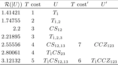
a fiducial vector for a symmetric, informationally com-plete positive operator valued measure (SIC-POVM) co-variant under the 3-qubit Pauli group. Some of these states were already classified as highly non-stabilizer by other means [32]. In Fig.3we depict the robustness of a one-parameter family ofm-qubit states, form∈ {1,2,3}. From this figure we can read offR(|H⊗2i)<R(|CSi)< R(|H⊗3i) andR(|H⊗3i)<R(|CCZi)<R(|H⊗4i). We can also see that a doubly-controlled rotation of angle
θ=π/2—aCCS gate—would require at least 5T gates to implement.
By exploiting the Jamio lkowski isomorphism, as in e.g. [35,36], we can also investigate the robustness of op-erations. In particular, for every unitaryU ∈U(2n) we can associate a state|JUi= (11⊗U)Pj∈Zn
2|j, ji.
Max-imizing the quantity R(|JUi) tells us the most robust unitary operations. For a single qubit we numerically find the optimal unitary to be
U = √1 2
1 ei3π 4
e−iπ 4 1
!
, (54)
R(|JUi) =R(|H⊗2i) =
1 + 3√2
3 , (55)
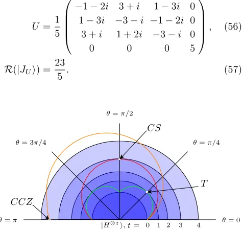
whereas optimizing over two-qubit unitaries we find
U = 1 5
−1−2i 3 +i 1−3i 0 1−3i −3−i −1−2i 0 3 +i 1 + 2i −3−i 0
0 0 0 5
, (56)
R(|JUi) = 23
5 . (57)
θ= 0
θ=π/4
θ=π/2
θ= 3π/4
θ=π
CCZ
|H⊗n
, n= 0 1 2 3 4
CS
T
t
[image:10.612.325.564.264.490.2]t
FIG. 3. Polar plot where the radial coordinate denotes robustness and the angular component represents the last entry in a m-qubit resource state (1, . . . , eiθ)T/2m/2.
Con-centric semi-circles correspond to robustness R(|H⊗ti) for t = 0,1, . . . ,4. Highlighted points correspond to resource states forT, CS and CCZ. We see that R(|H⊗3
i) is only slightly greater than R(|CSi), meaning that CS synthesis using 3T gates as in Fig. 1(c) of main text is optimal and no ancilla-assisted or non-deterministic strategy could be more parsimonious.
Interconvertability
Lower fromD(23) and (40) Lower fromR(|Ui) U∈ hCNOT, Ti Upper
R(|H⊗6
i) 3.1269 4.7031 T1CS24,35,45 4.9238
R(|H⊗7
i) 3.75592 5.5242 T4CS13,24,35,45 6.3523
R(|H⊗8i) 4.52157 5.7934 T
5CS12,35,45 8.1953
R(|H⊗9i) 5.4501 6.2625 T
1,2,3CS12,14,25CCZ345 10.555 R(|H⊗10
i) 6.5738 6.8995 T1CS12,23,14,25,45CCZ345 13.594
R(|H⊗11
[image:11.612.82.270.251.355.2]i) 7.9321 6.9255 T5CS23,24,45CCZ125,345 17.341
TABLE II. Bounds onR(|H⊗ti) for 6≤t≤11: The upper bound is given byR(|H⊗ti)≤ R(|H⊗jt2 k
i)R(|H⊗ lt
2 m
i) which holds because of submultiplicativity of robustness. The first lower bound derives from expression (23) usingD(|H⊗ti) = [D(|Hi)]t= h
1+√2 2
it
(40). The second lower bound corresponds to R(|Ui) whereU, provided in the column headedU ∈ hCNOT, Ti, is synthesizable over the CNOT+T gate set usingt T gates [23]. Clearly any suchU satisfiesR(|Ui)≤ R(|H⊗ti). Another way
of interpreting this column is to note that theseU are the most robust gates we know how to construct over the CNOT+T
gate set usingt∈ {6,7, . . . ,11}T gates. There are no five-qubitU ∈ hCNOT, Tithat require more than 11T gates.
R(|Ui) T cost U T cost′ U′
1.41421 1 T1
1.74755 2 T1,2
2.2 3 CS12
2.21895 3 T1,2,3
2.55556 4 CS12,13 7 CCZ123
2.80061 4 T1CS23
3.12132 5 T1CS12,13 6 T1CCZ123
TABLE III. Three qubit classification: All the three-qubit diagonal gates from the third level of the Clifford hierarchy can be classified by the robustness of the associated resource state|Ui=U|+i. The cost of synthesizing these gates over the Clifford+T gate set is provided. Two gatesUandU′with
the same robustness and differentT cost are equivalent via the construction described in connection with Eq. (7) of the main text.
equation (7);
T1,2CCZ345 8→6
−→T1,2CS35,45, (58)
T1,2,5CCZ345 8→7
−→T1,2,5CS35,45, (59)
T1,2,3,4CS23,24,34 7→6
−→T1,4CS24,34, (60)
CS12CCZ345 9→7
−→CS12,35,45, (61)
T5CS12,25CCZ345 9→7
−→T5CS14,25,35,45. (62)
These are all provably optimal in the sense that the T
cost on the right hand side is the minimum possible, as it is the smallest integertsatisfyingR(|Ui)≤ R(|H⊗ti).
We also make a brief comment on resource intervertability. Are there optimal transformations that con-vertn-qubit|φi tom-qubit |ψi,m6=n, withR(|φi) = R(|ψi)? At least one such transformation does exist. In the range 0≤θ≤arctan13, two copies of the equatorial state|φi= (|0i+eiφ|1i)/√2 have robustness
R(|φ⊗2i) = (2 sinφ+ sin 2φ+ cos 2φ+ 1)/2 but a measurement of Pauli operator ZY on|φ⊗2i, fol-lowed by a CNOT, creates the state|ψ±i|Y±i depend-ing on the ZY outcome, where |ψ±i has Bloch vec-tor ~r = (cos2(θ),sin(θ) cos(θ),±sin(θ)) hence ||~r||
1 = R(|ψ±i) =R(|φ⊗2i). Finding further examples of such transformations could find application in magic state preparation. The foregoing leads naturally to the ques-tion of asymptotic interconvertibility, much studied in the context of entanglement, where one seeks to maxi-mize the ratem/nin the limitn→ ∞of a stabilizer op-eration mapping|φ⊗ni → |ψ⊗mi. In this work we have dealt solely with deterministic gate synthesis but the ex-tension to probabilistic (depending on measurement out-comes) circuit synthesis is natural; the expected robust-nessE[R(|φi)] is now the relevant quantity to compare to e.g, R(|H⊗ni). Our choice to focus on synthesizing gates from the third level of the Clifford hierarchy was motivated by the fact that any measurement outcomes
[image:11.612.95.294.493.591.2]