Managing dose-, damage- and data-rates in multi-frame spectrum-imaging

White Rose Research Online URL for this paper: http://eprints.whiterose.ac.uk/128094/

Version: Accepted Version

Article:

Jones, L, Varambhia, A, Beanland, R et al. (10 more authors) (2018) Managing dose-, damage- and data-rates in multi-frame spectrum-imaging. Microscopy, 67 (S1). i98-i113. ISSN 2050-5698

https://doi.org/10.1093/jmicro/dfx125

© The Author(s) 2018. Published by Oxford University Press on behalf of The Japanese Society of Microscopy. All rights reserved. This is a pre-copyedited, author-produced PDF of an article accepted for publication in Microscopy following peer review. The version of record, Jones, L, et al.; Managing dose-, damage- and data-rates in multi-frame

spectrum-imaging, Microscopy, is available online at: https://doi.org/10.1093/jmicro/dfx125.

[email protected] https://eprints.whiterose.ac.uk/ Reuse

Items deposited in White Rose Research Online are protected by copyright, with all rights reserved unless indicated otherwise. They may be downloaded and/or printed for private study, or other acts as permitted by national copyright laws. The publisher or other rights holders may allow further reproduction and re-use of the full text version. This is indicated by the licence information on the White Rose Research Online record for the item.

Takedown

If you consider content in White Rose Research Online to be in breach of UK law, please notify us by

Managing dose-, damage- and data-rates in

multi-frame spectrum-imaging

Lewys Jones1,2,3*, Aakash Varambhia3, Richard Beanland4, Demie Kepaptsoglou5, Ian Griffiths3,6, Akimitsu Ishizuka7, Feridoon Azough8, Robert Freer8, Kazuo Ishizuka7,

David Cherns6, Quentin M. Ramasse5, Sergio Lozano-Perez3 and Peter D. Nellist3

1.

School of Physics, Trinity College Dublin, Dublin, Ireland 2.

Advanced Microscopy Laboratory, Centre for Research on Adaptive Nanostructures and Nanodevices, Dublin, Ireland

3.

Department of Materials, University of Oxford, Oxford, UK 4.

Department of Physics, University of Warwick, Coventry, UK 5.

SuperSTEM Laboratory, SciTech Daresbury Campus, Daresbury, UK 6.

University of Bristol, Bristol, UK 7.

HREM Research, Tokyo, Japan 8.

School of Materials, University of Manchester, Manchester, UK

* [email protected]

As an instrument, the scanning transmission electron microscope (STEM) is unique in

being able to simultaneously explore both local structural and chemical variations in

materials at the atomic scale. This is made possible as both types of data are acquired

serially, originating simultaneously from sample interactions with a sharply focused electron

probe. Unfortunately, such scanned data can be distorted by environmental factors, though

recently fast-scanned multi-frame imaging approaches have been shown to mitigate these

effects. Here, we demonstrate the same approach but optimised for spectroscopic data; we

offer some perspectives on the new potential of multi-frame spectrum-imaging (MFSI) and

show how dose-sharing approaches can reduce sample damage, improve crystallographic

fidelity, increase data signal-to-noise (SNR), or maximise usable field of view. Further, we

discuss the potential issue of excessive data-rates in MFSI, and demonstrate a

Spectrum imaging, non-rigid registration, beam damage, dose-rate, data compression

The aberration corrected scanning transmission electron microscope (STEM) can now

routinely image crystalline specimens at atomic resolution. Of the imaging modes available

the relative ease of interpretation of the annular dark-field mode (ADF) makes this a popular

choice, offering thickness / atomic-number type contrast. However, the mixed

thickness-composition contrast introduces some ambiguity in heteronuclear samples, so for

composition studies either energy dispersive x-ray analysis (EDX) or electron energy-loss

spectroscopy (EELS) are added to many STEMs. Unfortunately, the collection efficiency of

these signals is around 100 and 10,000 times weaker respectively compared with

imaging [1].

While spectrometer hardware is improving gradually, little has changed in the way

that spectrum images (SI) are recorded since their introduction [2,3]. For most studies, the

poor collection efficiency means the signal-to-noise ratio (SNR) limits the clarity of results.

There are three common approaches pursued to increase the SNR of elemental maps;

increasing the beam current, increasing the pixel dwell-time or the installation of a higher

collection efficiency detector or spectrometer. However, the first two approaches have

significant drawbacks. Increasing beam current can rapidly cause sample damage [4] or

accelerate carbon contamination, while scanning slower risks introducing scanning

increase the beam current (such as in monochromated systems), while increased

dwell-times make recording larger fields of view prohibitively time consuming for the operator.

Lastly, spectrometer upgrades may not be possible, for example due to objective pole-piece

space restrictions or prohibitive cost.

Thanks to recent developments in the robust registration of serial scanned image

data [6,7], multi-frame spectrum-image (MFSI) data can now be equally successfully

reregistered [8,9]. Multi-frame experiment design frees the operator from using slow scans

and high-probe currents to realise acceptable SNRs. Instead, the required signal is built up

from a series of faster and individually lower dose scans; specimen drift is greatly reduced,

as is in many cases beam-damage, while the redundant set of complimentary ADF images

allows for scanning distortion to be compensated without the need for specially designed

instruments [10].

Since the term ‘spectrum imaging’ was introduced in the 1980s, continuous

improvements in instrumentation and computer power have been realised. However, MFSI

inevitably generates a far greater data-rate than conventional single scan approaches.

Approaches to reduce EELS-SI data-rate based on compressed-sensing have been proposed,

but these require additional hardware such as grating apertures and complex

synchronisation [11]. As data-rates increase, there is wisdom in returning to those

suggestions made before computing power was so advanced. Previous approaches have

considered data-binning [2], or neighbour-difference approaches [12]; however, these may

be unacceptably lossy or offer only limited storage savings. Here we seek to implement

some approach which requires no new hardware and instead makes use of the prior

and about how experimentalists ultimately process the data (with background fitting and

integration) to produce various 2D maps. We present a modification of the method

proposed in [2], but dividing SI data in the energy domain into blocks, some of which receive

no compression where fine measurements are needed (such as the zero-loss peak (ZLP)

position or fine-structure edges), and others which are down-sampled after some

appropriate noise reduction.

In summary, in this work we make use of the ability to acquire, store, and robustly

align MFSI data to introduce a new free-parameter into the operator’s experiment design.

We present five separate studies, each highlighting different aspects of this new approach

that probe the performance of the method. In this work we:

1. present a fixed-electron-dose study, comparing the sample-damage of a

beam-sensitive specimen with and without multi-frame dose-fractionation,

2. demonstrate (for a beam-tolerant specimen) the accumulation of SNR, and the utility

of digital super-resolution in spectrum imaging,

3. show a sub-20pA atomic-resolution EDX mapping example, through the combined use

of MFSI alignment and image template-matching (TM),

4. reveal through the use of multivariate statistical analysis (MSA), the minimum dose

required to capture the information-content of SI data, and

5. describe a new highly-efficient compression routine to minimise the

In this work, several different descriptors of sample-beam exposure are used; for

clarity, these are defined explicitly here. Dose-per-frame is expressed in units of electrons

per-square-Angstrom (e-Å-2). The total-dose, i.e. the entire electron-dose, is also expressed in

units of electrons per-square-Angstrom (e-Å-2) and is simply the dose-per-frame multiplied

by the number of frames in the series. Dose-rate is the total-dose divided by the duration of

the corresponding exposure, with units of electrons per-square-Angstrom per-second (e-Å-2s

-1

); this is either calculated as the dose-per-frame divided by the frame-time (number of

frame pixels multiplied by the dwell-time), or as the total-dose divided by the total

series-time. A final commodity which is of merit for fast-scan multi-frame acquisitions where the

probe is always moving, is the instantaneous pixel charge delivered by the passing probe (in

electrons), and is calculated as the beam current multiplied by a single pixel dwell-time.

Samples and Hardware Configurations for each Test

Three unique instruments were used across the studies presented here. For the

fixed-dose study (test 1), the sample used was Pb2ScTaO6 prepared for STEM imaging by ion

beam milling. This material exhibits incomplete long-range ordering on the Sc:Ta sublattice.

Two data-sets were recorded using a doubly-corrected JEOL ARM200F 1Å probe of 74pA with a convergence of 30mrad). Simultaneous hardware synced spectra were recorded

using a Gatan Quantum GIF and Oxford Instruments X-max 80mm2 detector. A single

256x256 probe-position spectrum image with a dwell-time of 0.01 s/pix was recorded, and

for comparison five separate spectrum images with a dwell-time one fifth of the single frame

(0.002s/pix), i.e. at equal total-electron-dose and equal dose-rate. Imaging was carried out

To demonstrate SNR accumulation, digital super-resolution, and EELS SI

data-compression (test 2 & test 5), an A-site deficient perovskite, Nd0.6Ca0.1 0.3TiO3 (where

denotes A-site vacancies), was used. The sample was prepared by conventional crushing

(pestle and mortar) and drop cast on a standard 3mm lacy-C film support; the sample was

previously characterised and discussed in [13]. ADF imaging and atomically resolved EELS

mapping were performed using a NION UltraSTEM100 MC dedicated STEM equipped with a

Gatan Enfinium ERS spectrometer optimised with high stability electronics. The microscope

was operated at 60kV with the probe forming optics configured to form a 1Å probe

(full-width at half-maximum), with a convergence semi-angle of 31mrad yielding a probe current

of 110pA. The dataset presented here comprises of eight spectrum images with lateral

dimensions of 60x94 pixels Å -size) acquired consecutively using a dwell time of 0.001s/pix and 16 x 16 subpixel scanning, into a spectrometer entrance aperture with a

48mrad semi-angle. The total acquisition time per SI frame was 1min 15s, including

overheads. No drift compensation was applied during the acquisition or between SI frames.

For the MFSI, TM, and data compression (tests 3-5), an Ag2ZnSnSe4 (AZTS) sample

was prepared from a stoichiometric mix of pure elements annealed at up to 510°C for 46

days in sealed ampoules at 10-6 torr, then slow-cooled at 3°C/hour to room temperature

achieving grain sizes of up to several micrometers. One extended single-crystal was imaged

which at the edge was EELS to be 20-30nm thick but extended laterally for several hundred nanometers. Annular dark-field (ADF) imaging and EDX mapping was

performed using a JEOL ARM200CF equipped with a single Centurio 100mm2 EDX detector. A

17pA beam at 200kV was used to record 230 simultaneous ADF-EDX SI pairs at

approximately 41s. This gives a dose-per-frame of 3.44 x 105 e-Å2. Images across the single

crystal were recorded in sets of 10-frames, each set from a virgin area of crystal.

Data Acquisition

To reduce operator burden and maximise experimental throughput, an interactive

graphical script was written in Digital Micrograph where image-SI pairs are recorded,

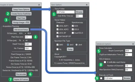
numbered, and saved to disk automatically. Figure 1 shows the appearance of the developed

user interface.

Figure 1. Interactive graphical user interface for the streamlined data acquisition, numbering and saving. The numbered

items are described in the main text.

Here the user first indicates the save-path for the microscope session (1), the data

writing overhead time, the image and SI signals to record, and for the SI whether

file-compression should be used; after that numbered sub-folders may be created for each new

region-of-interest (ROI) without leaving the main work-flow (2). After this the user works

interest (3). With the position and size of the ROI set, the user specifies the required

pixel-size (4); this is contrary to the microscope’s built-in workflow where the number of pixels is

treated as the free parameter. Here the number of pixels is automatically determined for the

user to deliver them a specific pixel size, with a minute expansion of the ROI size if

necessary. In the ‘Advanced Setup’ menu, the user specifies the STEM probe current and the

time-overhead of initialising communications to the DigiScan unit (5).

With the SI parameters set, the user is presented with estimates of the frame-time,

series-time and their associated electron-dose estimates. If the user adjusts either the size of

the ROI, the pixel-size, dwell-time or number of frames, the time and dose estimates can be

re-evaluated (6). This gives the user an indication of the practicability of their set conditions

before the acquisition is started. Detailed spectrometer settings such as EELS dispersion,

offsets and exposure times are handled as usual in the Gatan menus. The electron-dose for

the entire series including all communication and fly-back overhead times is also shown; this

is often ignored but may be crucial for studies on beam sensitive materials.

The image and SI series is then recorded (7) with each data being saved to disk and

closed from memory as it is completed. If the sample remains undamaged, and further SI

frames are desired (for example, to extend the series to increase SNR), the ‘acquire SI

frames’ button can simply be pressed again and further SI frames will be added to the same

sub-folder. This can be repeated as required until the user presses the button to create and

move to the next numbered sub-folder for the session. In advanced settings, the user can

select other useful automations; such as to step the EELS spectrum along the camera

between SI frames by incrementing the drift-tube voltage (8) (similar approaches have been

by Wang et al [16] to improve dark-reference/spectrum quality), or to execute a custom

script on completion (9). Such a custom script might for example: drop the magnification

10,000x (reduces dose-rate by 108), close the beam entirely (on systems where this is

available), or to send an email to the operator that the series is complete [17].

Data Processing

Using the ADF images acquired alongside the SI data, the image-alignment and

scan-distortion corrections were diagnosed in post-processing following the method in [6]. This

approach allows the operator to choose to record scan frames with larger fields-of-view than

would otherwise be possible, increasing the accessible field-of-view and reducing the need

to chase features by manual adjustment during acquisition [18]. The shift-vectors between

frames, and the non-linear 2D distortion-fields within each frame are stored at the end of

this calculation. These data are then used to correct for the equivalent shifts and distortions

in the SI data conceptually similar to the method followed by Yankovich et al. [9], but instead

utilising specific prior knowledge that the STEM is a scanning probe instrument, to improve

the alignment speed, robustness and accuracy [6]. Moreover, the method deployed here

differs from this earlier work, in that the spectrum-image rearrangement and restoration

steps (steps 3 and 5 in Figure 3 of reference [9]) are avoided to improve calculation speed

and memory use. In the present work, each SI is operated on in series; where within each

given SI, every spectral-channel is corrected by the distortion-field for that scan, before

being added to a running summation SI-volume. This approach means that at no time do the

SI data need to simultaneously stored in computer RAM, all memory needed can be

both the field-of-view and the number of frames in the SI acquisition. The significance of this

serial-SI processing will be discussed further in the context of data-compression later on.

To perform the template-matching, where repeating features are identified across

the view [19], a region-of-interest (ROI) is first drawn to highlight a motif within the image.

In this case, the selected ROI is 2-3 unit-cells in size and is then cross-correlated across the

full field-of-view to identify all the repeat units of that motif. These repeats are then

themselves cropped to form an image series for averaging. Where a corresponding SI exists,

the same regions from this can also be cropped and averaged further improving SNR [8,20].

Where an image and SI series exist, the image motif can be automatically searched

throughout the entire image series (folder), noting the frame number and x-y position

before repeating the same across the SI series.

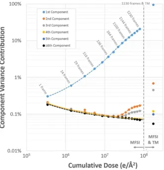
For test 4, the inspection of data information-content by multivariate statistical

analysis (MSA), Scree plots were calculated using the Hyperspy package after singular value

decomposition (SVD) [21], for increasing cumulative doses. With these, the percentage

contribution to the data variance is plotted, where the number of components with a

variance contribution visibly greater than the Scree-plot background is an indication of the

ease of separability between genuine signal and random noise [22].

For test 5, to compress the EDX file-size, only non-zero data are stored of SI

voxels) noting their position in voxel order and their (integer) x-ray photon count. This data

is read and restored to the full dimensions on decompression. To reduce EELS spectra

file-size, the over-redundant nature of each spectrum is exploited. First, the energy-domain is

divided into regions by the user which are to be used for broad background determination

regions of interest, these are often known from say an earlier point spectrum before any

mapping is performed. Next, within only the spectral-blocks which are to be down-sampled,

extreme outliers are removed from the data (by say median filtering) and random

uncorrelated noise (by principal component analysis (PCA) but with several tens of

components preserved), before being smoothed in the energy dimension only by a kernel

whose width in channels is equal to the down-sampling. These de-noised data are then

down-sampled, and the reduced size SI data are stored after taking their natural logarithm.

To further reduce storage size, the data are rounded to their first four significant figures. To

decompress the data back to the full dimensionality, the missing values are linearly

interpolated, before restoring the magnitude by raising them by the natural exponent. This

linear interpolation before raising by the exponent exploits the power-law decay often found

in background regions for thin samples (with no multiple scattering). This is an improvement

over the simple binning proposed in [2], and prevents long flat, or even linear blocks, being

restored in the decompressed spectra. Our proposed compression is customisable, is locally

lossless in the regions where no down-sampling is performed (for example for fine structure

studies, or ZLP drift tracking), and allows for significant data-savings in less important regions

of the spectrum. The only additional data to store during the compression is the

channel-number/down-sampling pairs as annotated in Figure 8.

To produce elemental maps, power-law backgrounds were fitted before the EELS

edges, and for the EDX maps characteristic x-rays were integrated after subtracting a linear

background. In all comparisons, the same backgrounds and peak/edge integrations were

The results presented follow the five themes listed above.

1 – Reduced Damage with Fast Scanning

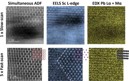
Figure 2 shows the fixed-dose comparison between conventional and MFSI

approaches. As the beam current remained fixed for this test, and as 5-frames at 5x speed

were recorded, the dose-rate (1.03 x 10 e-Å-2s-1) and total-dose (6.7 x 107 e-Å-2) were

necessarily equal.

Figure 2. Fixed total-dose comparison of single-scan and multi-frame strategies. Figure shows the ADF image (left), the Sc

map measured by EELS (centre), and the Pb EDX map (right). The dashed-line indicates the position of the anti-phase

boundary.

The ADF of the conventional single frame acquisition immediately shows the

beam-damage and scanning-distortions which arise from using the slower scan speed. The

fast-scanned, distortion-corrected, and averaged ADF image however shows both improved SNR

and less distorted lattice planes as expected [23]. The location of the anti-phase boundary is

-edge EELS maps show an improvement from 2.1 to 5.1 with the Sc positions relating directly

with the ADF image. EDX maps are less clear but in the multi-frame average spectrum image

the Pb lattice begins to become apparent. As sample damage is reduced so drastically, more

frames could have been recorded to improve SNR further if desired. This was not done here

to allow a fair comparison at fixed total dose conditions.

This test indicates that in addition to discussing a sample’s critical dose, or

dose-rate [24], we should perhaps also evaluate the instantaneous pixel-charge, as it is only the

third of these quantities which is different in the fast MFSI acquisition. For this example, the

pixel charge was reduced from 4.62 x 106 e- to 9.24 x 105 e- by changing to the MFSI regime.

2 – Improving SNR, Detectability & Sampling (Digital Super-resolution)

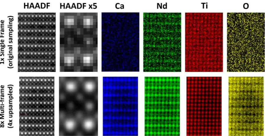
Figure 3 shows both a single ADF and EELS-SI frame (top row) displayed with

the as-acquired pixel sampling. While the raw data were acquired well above the

Nyquist frequency capturing all the resolvable information Å Å probe), the resulting maps appear rather pixelated. Instead of the temptation of

increasing the sampling during the acquisition (with the associated dose and

frame-speed implications), we employ digital super-resolution during the

post-processing [25]. The image and SI data were up-sampled by a factor of 4 before rigid

and non-rigid alignment [6]. It is essential that this up-sampling is performed before

alignment for any digital super-resolution benefit to be realised. The bottom row

Figure 3. Example of combined use of multi-frame SNR accumulation, and digital super-resolution to increase pixel density.

Image / SI field of view = 40 x 63nm

While some lattice information is visible in the single-frame EELS maps for the Nd and

Ti signals, the SNR is very poor; Ca and O maps reveal no periodicity. Upon averaging all four

signals are clearly resolved. As in previous studies full intermixing between the Ca and Nd

was confirmed. It should be noted that there is some small loss of image-width as a result of

cropping following the image alignment (as a result of stage drift), as well as some early

signs of damage beginning to appear, especially on the oxygen lattice. This damage may

have begun earlier during the operator refocussing and stigmation just before the start of

the acquisition whose cumulative effects should be considered in future low-dose studies.

3 – Combining MFSI and Template Matching for sub-20pA EDX Mapping

Image template-matching (TM) with crystallographic prior knowledge has

been shown to improve image quality [19]; and further, when exploiting

rotational-symmetry has previously been shown to yield atomic resolution EDX maps from

acquisition and the analysis, only translational (and not rotational) symmetry was

assumed.

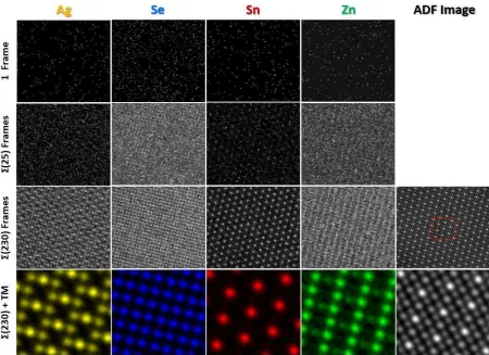
Figure 4. Signal accumulation over a 230-frame EDX series. Far right column shows the aligned ADF image corresponding to

the 230-frame series and (highlighted in red) the ROI used for the template-matching (the motif).

Figure 4 shows extracted maps corresponding to the four elements present

for a single-scan, after aligning 25 frames, and after summing across the full

230-frame acquisition. These correspond to total-doses of 3.4 x 105, 8.6 x 106, and

7.9 x 107 e-Å-2 respectively.

After this the ADF ROI shown far bottom-right was used to identify 112

repeat motifs for further SNR accumulation (Figure 4 – bottom row). The effective

equivalent dose then of the TM EDX maps is 230x112 times the original single frame

processing) a two-dimensional equivalent of the previously proposed 1D smart

line-scans [26], where dose is shared across equivalent positions. In these

template-matched EDX maps, the atomic columns are now clearly resolved and differences in

the occupancies are readily visible in the Ag and Zn maps; all the while using only a

17pA STEM probe. Using TM to deliver such high SNR, it may be possible to

determine interface intermixing profiles more accurately without needing to

increase sample-thickness or beam current [27], or to study the x-ray emission from

individual x-ray lines separately [28]. Moreover, TM performed in real-space opens

the possibility to map point defects/dopants that would be impossible by Fourier

based techniques.

4 – Quantitative Evaluation of Information Content

In this section we continue the analysis of the experimental data from the sample

used in section 3 – to determine the information content of the recorded spectra. When

decomposing spectra using PCA, a Scree plot is used to show the contribution to the

variance described in each component. In a decomposition of spectra we expect

n-components, though in practice far fewer of these orthogonal components contain useful

information – this is the basis of the noise reduction. In an ideal situation, the decomposition

s described in as few components as the sample complexity requires.

Figure 5 shows the Scree-plot data as a function of increasing cumulative electron

dose which the sample received. At the lowest dose (single-frame, 3.4 x 105 e-Å-2),

information is shared almost equally amongst all components, which contain mostly noise.

relevant information and a cut-off for denoising can be determined. Further data points

represent the sum over the first 1, 4, 9, 16, 25, 36, 49, 64, 81, 100, 121, 144, 169, 196, and

230 frames [21]. A scree plot was also calculated for the template matched summation.

Figure 5. Information content, as evaluated by the component variance in the first 5 components, as a function of increasing dose. Components 6 and onwards represent the noise floor. The increasing dose-series is created by integrating increasing numbers of scan frames as labelled. The sum over the whole 230-frames with TM yields a final data-point (far right) with an

effective dose of 8.9x109 e-Å-2.

As the dose is increased (by summing more frames) the difference between this first

and other components becomes greater. From around 2.2 x 107 e-Å-2 (64 frames) the second

component becomes significant above the noise, then at 2.8 x 107 e-Å-2 (81 frames) the third,

and at 5.8 x 107 e-Å-2 (169 frames) the fourth. After template matching, 5 components were

clearly identifiable above the noise (6th onwards).

While dose-fractionation across n-frames was shown above to improve spatial

fidelity and reduce sample damage, it inevitably requires an n-fold increase in computer

storage. This situation is especially acute for the example given in Figure 4 where 230 EDX-SI

and ADF-image pairs were recorded. The total storage used for this one region of interest

was 70.3Gb (75.6 x 109 bytes). This becomes a significant burden both on EM-facility servers

but also in transmitting data to collaborators or to analysis PCs and for data-archival

purposes.

The solution here lies in the nature of EDX SI-data itself. At low electron-doses, these

files are mostly filled with zeros, while (because of the photon counting nature of the EDX

detector) the non-zero elements are filled with integer counts. Instead of storing the full 3D

arrays, massive storage savings can be realised by listing only the bins that contain non-zero

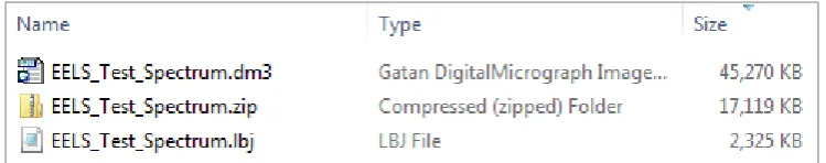
elements. Here we introduce such a listed-bin-journal file type (*.lbj) which records data in

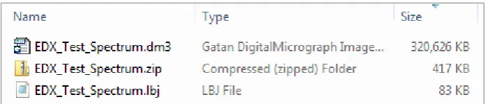
this sparse way. Figure 6 shows the first frame of the data from Figure 4 compressed from

both .dm3 > .zip, and from .dm3 > .lbj.

Figure 6. Example of the original and compressed EDX SI files as seen in Windows File Explorer. The compression ratio of the .lbj file is approx. 3900x and is a further 5x smaller than a simple .zip file.

The .lbj file is 3,905 times smaller which more than compensates for the acquisition

strategy of fractionating the dose across 230 frames. The result is also more than 5x smaller

than simply storing the data in a .zip archive. Unlike the >70GB raw data for this dataset, the

entire 230-frame EDX series after compression requires MB and can, for example, be

To benchmark the performance of the compression algorithm, the same process was

repeated for many SI example spectra from a variety of samples and beam currents, yielding

varying degrees of SI sparsity.

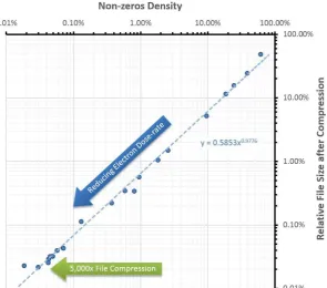
Figure 7. File compression results for increasingly low electron-dose EDX SI volumes.

Figure 7 shows that as the density of non-zero SI elements falls, the compression

approach followed here becomes more efficient as expected. For data with very few

non-zero elements the files are still compressed but less so. In the tests compressions of up to

5,000x were realized for the lowest dose data.

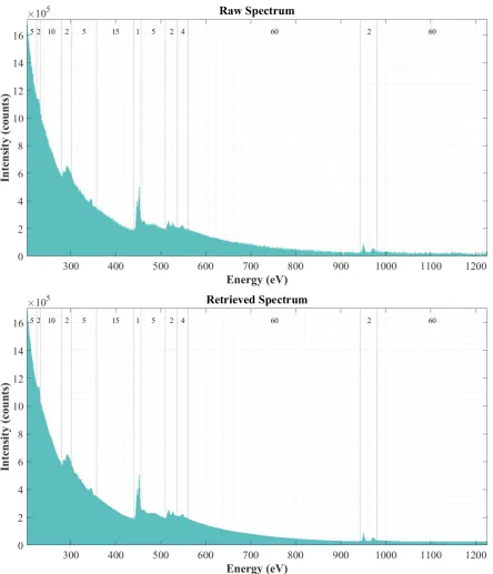
To evaluate the EELS data compression described in the Methods section, the MFSI

data presented in Figure 3 was compressed using blocks of down-sampling ranging from 1 at

Figure 8. Original EELS spectrum (top) corresponding to one SI of the data shown in Figure 3, and the equivalent spectrum after compression and decompression (bottom). Annotations across the top of each plot show the local down-sampling used

to compress that spectral block. The residual between these two figures is shown in the Appendix.

In the many-featured spectral example shown above, the EELS SI files were reduced

in size by more than 94 19.4x smaller); for the 8-SI series shown in Figure 3, this

corresponds to a reduction from 353MB to 18.4MB. For the Pb perovskite example shown in

Figure 2, whose more simple EELspectra contained only Sc and O edges, the compression

Figure 9. Example of the original and compressed EELS SI files as seen in Windows File Explorer. The compression ratio of the .lbj file is approx. 19.4x and is a further 7.4x smaller than a simple .zip file.

Similar to the EDX example presented earlier, this more than compensates for the

eight frames of the MFSI acquisition, or alternatively would facilitate increasing the

field-of-view significantly, or storing the final aligned spectrum where 4x digital super-resolution has

been used (16x more pixels).

As yet, there is no clear consensus in the literature as to whether total-dose or

dose-rate is most responsible for electron beam damage. However, studies particularly on oxide

materials present evidence that there exists some threshold dose-rate, below which damage

is not observed [24,29]. In this work, we do not seek to settle this argument, but rather

through the introduction of a practicable MFSI approach, we present the user with the tools

to optimise their individual experiments, introducing the flexibility to fractionate dose across

frames. Moreover, our first experiment with the Pb-perovskite indicates that, even when

both total-dose and dose-rate are fixed, notable differences still exist based on acquisition

design. Here the unit of instantaneous pixel charge is the only one which changes and

further investigation of this is left to future work.

We saw from test 1, from a sample damage perspective, that it is by far preferable to

record n-frames than one frame n-times slower. In addition to introducing the number of

digital super-resolution (as used in test 2) allows for sub-pixel scanning distortions to be

more precisely compensated, and for the operator to produce finely sampled chemical maps

(suitable for line-profile, peak-fitting etc.) without the need to physically scan the sample at

such a high pixel density. So long as the raw experimental data is recorded above the

Nyquist frequency (generally >2x is sufficient), then the resolvable information will be

encoded in the recorded data. However, investigators generally prefer to present images far

more finely sampled than this. In test 2, 4x digital up-sampling was used to improve the pixel

density of the resultant chemical maps. If this density of pixels were to have been recorded

experimentally, this would represent a 16x increase in experimental time and

beam-exposure. In this way digital super-resolution allows the operator to optimise the acquisition

to operate close to the Nyquist information limit, but to still produce finely sampled images

suitable for detailed onward analysis. Moreover, recoding the experimental images at the

minimum appropriate sampling is not only beneficial from a dose perspective but is also

more practical for data-storage.

In test 3, we demonstrated that atomic-resolution EDX maps of repeating structures

(here a single crystal), can be obtained using a sub-20pA beam more commonly associated

with high-resolution imaging conditions than for analytical work. This is made possible, in

part, by the extremely low dark-noise of the EDX detector and the ease of automatically

aligning large multi-channel data volumes. The SNR expected in the chemical maps can be

predicted using a chart such as that from Wenner et al. [8], and this is reproduced in the

appendix for the material used here. As the TM approach does not use any real-space

smoothing or Fourier filtering, it preserves the maximum possible resolution and does not

Singular value decomposition (SVD) and other blind source separation techniques are

powerful statistical techniques for the reduction of noise in spectrum imaging data [30].

However, one often challenging aspect of this is determining the appropriate number of

statistical components which should be used to decompose the data; too few and some

important information may be missed (or under-described), while including too many

components needlessly increases uncorrelated noise. The number of components is usually

determined from analysing so called ‘Scree plots’. However, for low SNR data, these rarely

show the abrupt corner needed for an unambiguous determination and other issues may

arise [31]. In this work, we observed that the separability of the orthogonal components

became increasingly clear for higher doses. Gradually a second, third, and fourth component

became significant rising out of the noise floor. After TM, the effective dose-accumulation

yielded a sufficiently high SNR that eventually 5 components were observable; and while the

material only contained four species, we attribute the need for this 5th eigenvector as being

necessary to describe the two different local (de)channelling environments for the two

non-equivalent silver sites. A more extensive simulation study is now underway to explore this

further as a function of specimen thickness.

The data compression approaches described above for EDX and EELS not only allow

for SI data to be compressed at the end of every SI-frame acquisition before saving to disk,

but also is compatible with the serial nature of the SI distortion correction approach used in

the SmartAlign algorithm [6]. In this approach, each SI can be read from disk and

decompressed just as it is needed, scan-corrected, added to the running-summation and

then cleared from RAM without ever needing to be written to disk in its uncompressed form.

network (or write it to a hard-drive), and decompress it than to transmit the full sized raw

data. For the EDX compression, we find that the proposed compression performance

actually increases as the dose-rate is reduced, offsetting the increased number of frames

needed to accrue sufficient signal. For the EELS compression, while it is a prerequisite that

the user must have some prior knowledge about the spectrum they will record, this is not a

substantial limitation, as the user is already required to setup their spectrometer for the

expected elements to be mapped, and will have likely already recorded some point-spectra

in preparing the exposure conditions of their CCD. To evaluate the performance of the

proposed compression further, the individual SI data shown in Figure 3 were compressed,

stored, decompressed and aligned; this was compared with data which were just directly

aligned with no compression. For the data where compression was used in the

spectral-regions for background determination, we actually observed an improvement in the SNR of

the extracted maps (see appendix). This observation is consistent with the work of

Spiegelberg et al. [32] and can be attributed to a more robust extrapolation of the

background in turn yielding less noisy elemental-maps.

Where the use of large fields-of-view, de-scan errors, or environmental instabilities

cause energy drifts across the EELS spectrometer, these should ideally be corrected before

the down-sampling compression [33,34]; this ensures the optimal size and position of the

down-sampling blocks.

Future possibilities for MFSI development exist in the hardware, software, and choice

Though the dark-noise of EDX spectrometers is very low, the same cannot be said of

the current generation of EELS cameras. Previously, albeit for image data, we have explored

systematically how increasing fractionation of a fixed dose can ultimately lead to signals that

are too noisy to register [23]; we expect a similar trend to be true for EELS MFSI where

increasing fractionation delivers no further benefit. This should be revisited in the future

when the new generation of electron counting cameras (with greatly reduced dark-noise)

become more available on spectrometers [35].

In software, the over-redundant nature of the MFSI also provides opportunities for

energy-domain realignment to counter energy drift in the EELS spectrometer. This is rarely

an issue in EDX, but electro-magnetic distortions, or power-supply fluctuations in the

instrument can lead to apparent fluctuations in energy-loss [34]. The multi-frame methods

described above are eminently compatible with proposed corrections for both energy-drift

stability (or de-scan effects) [33,34,36], and approaches to remove systematic noise from the

reference data used by stepping the spectrum across the CCD using the electrostatic

drift-tube to reduce systematic artefacts that may otherwise arise from using summed

spectra [14]. Where a ZLP is included in the spectrum (or with dual-EELS acquisition) the

energy domain can be realigned before spatial alignment and spectral summing. This

alignment minimises any loss of energy-resolution upon summing and allows users to

achieve the fullest performance of the new generation of monochromated systems. A similar

approach can also be followed to counter the energy-offset resulting from imperfect

post-specimen de-scan which causes the electrons to enter the spectrometer slightly off-axis.

While not the focus of this work, this is ideally suited to be incorporated in the automated

While the ability to reduce probe-current affords operators great hope for imaging

beam-sensitive materials, it also opens possibilities for studying intrinsically weak signals

from beam-robust samples where currently maps are often coarsely sampled and somewhat

noisy. These might include weak EELS phonon-spectroscopy [37], cathodo-luminescense

(CL) [38], electron beam induced current (EBIC) [39], or electromagnetic circular di-chroism

(EMCD) [40]. We hope to explore each of these opportunities in future works.

Using multi-frame spectrum imaging we have shown that for a fixed electron budget,

sample-damage can be reduced while simultaneously improving spatial precision. We have

shown that with increasing electron exposure over several frames, SNR can be accumulated

with no loss of spatial resolution resulting from scanning distortions; and we have shown

how combining template-matching with MFSI it is possible to obtain atomic resolution EDX

maps with a sub 20pA beam current. We have shown that the incorporation of digital

super-resolution (pixel up-sampling before alignment) allows users to obtain the finely sampled

chemical maps required without overly dense pixel-sampling at the point of acquisition.

To accommodate the inevitable increase in rate that MFSI brings, novel

data-compression techniques were introduced where even for complex EEL spectra, file size

, while remaining locally-lossless around fine spectral details of interest. For EDX the sparsity of low-dose SI allowed for even bigger data-savings

It is envisaged that our streamlined approach to data-acquisition,

compression/storage, and non-rigid realignment will facilitate a step-change in the scope of

experiment design for STEM spectroscopy.

This research was financially supported by the European Union Grant Agreement

312483 - ESTEEM2, JEOL UK Ltd and Johnson Matthey. Tests 3-5 were performed using the

‘South of England Analytical Electron Microscope’ at the University of Oxford, supported by

EPSRC grant code EP/K040375/1. L.J. would like to thank Mr. Haruki Tomioka (HREM

Research, Tokyo) and Dr Harura (Kyoto University) for their helpful discussions. SuperSTEM

is the U.K. National Facility for Advanced Electron Microscopy, supported by the Engineering

and Physical Sciences Research Council (EPSRC).

The research described here has been partially supported by HREM Research (Tokyo)

and aspects of this research will be made available as part of a commercial software plug-in

for the Digital Micrograph software. A free version of the SmartAlign code (in the Matlab

language) can be found at www.lewysjones.com .

:

[1] D. B. Williams and C. B. Carter, Transmission Electron Microscopy, 2nd ed. (Springer, 2009).

[2] C. Jeanguillame and C. Colliex, Ultramicroscopy 28, 252 (1989).

[3] J. A. Hunt and D. B. Williams, Ultramicroscopy 38, 47 (1991).

[4] R. Egerton, P. Li, and M. Malac, Micron 35, 399 (2004).

[6] L. Jones, H. Yang, T. J. Pennycook, M. S. J. Marshall, S. Van Aert, N. D. Browning, M. R. Castell,

and P. D. Nellist, Adv. Struct. Chem. Imaging 1, 8 (2015).

[7] B. Berkels, P. Binev, D. A. Blom, W. Dahmen, R. C. Sharpley, and T. Vogt, Ultramicroscopy 138,

46 (2014).

[8] S. Wenner, L. Jones, C. D. Marioara, and R. Holmestad, Micron 96, 103 (2017).

[9] A. B. Yankovich, C. Zhang, A. Oh, T. J. A. Slater, F. Azough, R. Freer, S. J. Haigh, R. Willett, and

P. M. Voyles, Nanotechnology 27, 364001 (2016).

[10] K. Kimoto, T. Asaka, T. Nagai, M. Saito, Y. Matsui, and K. Ishizuka, Nature 450, 702 (2007).

[11] A. Stevens, L. Kovarik, H. Yang, Y. Pu, L. Carin, and N. D. Browning, Microsc. Microanal. 22, 560

(2016).

[12] J. A. Hunt and D. B. Williams, Ultramicroscopy 38, 47 (1991).

[13] F. Azough, D. M. Kepaptsoglou, Q. M. Ramasse, B. Schaffer, and R. Freer, Chem. Mater. 27,

497 (2015).

[14] M. Bosman and V. J. Keast, Ultramicroscopy 108, 837 (2008).

[15] V.-D. Hou, Microsc. Microanal. 15, 226 (2009).

[16] Y. Wang, M. R. S. Huang, U. Salzberger, K. Hahn, W. Sigle, and P. A. van Aken, Ultramicroscopy

184, 98 (2018).

[17] B. Schaffer, How to Script... Digital Micrograph Scripting Handbook (2017).

[18] T. C. Lovejoy, Q. M. Ramasse, M. Falke, A. Kaeppel, R. Terborg, R. Zan, N. Dellby, and O. L.

Krivanek, Appl. Phys. Lett. 100, 0 (2012).

[19] S. Hovmöller, Ultramicroscopy 41, 121 (1992).

[20] M. Haruta, Y. Fujiyoshi, T. Nemoto, A. Ishizuka, K. Ishizuka, and H. Kurata, in (2017).

[21] F. D. La Peña, T. Ostasevicius, V. T. Fauske, P. Burdet, P. Jokubauskas, M. Nord, E. Prestat, M.

Sarahan, K. E. MacArthur, D. N. Johnstone, J. Taillon, J. Caron, T. Furnival, A. Eljarrat, S.

Mazzucco, V. Migunov, T. Aarholt, M. Walls, F. Winkler, B. Martineau, G. Donval, E. R.

Chang, DOI:10.5281/ZENODO.583693, (2017).

[22] S. Pack, Factor Analysis in Chemistry, 2nd ed. (Wiley, 1991).

[23] L. Jones, S. Wenner, M. Nord, P. H. Ninive, O. M. Løvvik, R. Holmestad, and P. D. Nellist,

Ultramicroscopy 179, 57 (2017).

[24] A. C. Johnston-Peck, J. S. DuChene, A. D. Roberts, W. D. Wei, and A. A. Herzing,

Ultramicroscopy 170, 1 (2016).

[25] G. Bárcena-Gonzálaz, M. P. Guerrero-Lebrero, E. Guerrero, D. Fernández-Reyes, D. González,

A. Mayoral, A. D. Utrilla, J. M. Ulloa, P. L. Galindo, G. Bárcena-González, M. P.

Guerrero-Lebrero, E. Guerrero, D. Fernández-Reyes, D. González, A. Mayoral, A. D. Utrilla, J. M. Ulloa,

and P. L. Galindo, J. Microsc. 0, 1 (2015).

[26] K. Sader, B. Schaffer, G. Vaughan, R. Brydson, A. Brown, and A. L. Bleloch, Ultramicroscopy

110, 998 (2010).

[27] S. R. Spurgeon, Y. Du, and S. A. Chambers, Microsc. Microanal. 1 (2017).

[28] J. S. Jeong and K. A. Mkhoyan, Microsc. Microanal. 22, 536 (2016).

[29] N. Jiang and J. C. H. Spence, Ultramicroscopy 113, 77 (2012).

[30] N. Bonnet, N. Brun, and C. Colliex, Ultramicroscopy 77, 97 (1999).

[31] S. Lichtert and J. Verbeeck, Ultramicroscopy 125, 35 (2013).

[32] J. Spiegelberg, J. Rusz, K. Leifer, and T. Thersleff, Ultramicroscopy 181, 117 (2017).

[33] Y. Sasano and S. Muto, J. Electron Microsc. (Tokyo). 57, 149 (2008).

[34] K. Kimoto and Y. Matsui, J. Microsc. 208, 224 (2002).

[35] J. L. Hart, A. C. Lang, A. C. Leff, P. Longo, C. Trevor, R. D. Twesten, and M. L. Taheri, Sci. Rep. 7,

8243 (2017).

[36] K. Kimoto, K. Ishizuka, T. Asaka, T. Nagai, and Y. Matsui, Micron 36, 465 (2005).

[37] C. Colliex, M. Kociak, and O. Stéphan, Ultramicroscopy 162, A1 (2016).

[38] M. Kociak and O. Stéphan, Chem. Soc. Rev. 43, 3865 (2014).

Cells 150, 95 (2016).

[40] J. C. Idrobo, J. Rusz, J. Spiegelberg, M. A. McGuire, C. T. Symons, R. R. Vatsavai, C. Cantoni, and

A. R. Lupini, Adv. Struct. Chem. Imaging 2, 5 (2016).

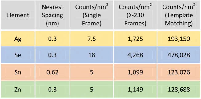
EDX SNR-Spacing Analysis

Following the method of Wenner at al. [8], (who operate an identical microscope to

the one used for the EDX template matching in this study), the number of characteristic

x-rays per square nanometre expected to be required for various projected atomic-column

spacing’s were evaluated.

Table 1. Calculated x-ray yields for the four species and their lateral-separation in projection.

Element Nearest Spacing (nm) Counts/nm2 (Single Frame) Counts/nm2 ( -230 Frames) Counts/nm2 (Template Matching)

Ag 0.3 7.5 1,725 193,150

Se 0.3 18 4,268 478,028

Sn 0.62 5 1,099 123,076

Zn 0.3 5 1,149 128,688

This experiment design tool is a descriptor which allows the operator to predict

whether an experimental series will contain enough SNR even before the NR-alignment of

Figure A1. Simulation of the appearance of the expected EDX maps with variable characteristic x-ray signal and projected atomic-column spacing (method described in [8]). Filled circles represent the experimental points from the results discussed in the main body.

Figure A1 shows that consistent with the results shown in Figure 4, it is not

expected that the single-frame EDX would be resolvable (due to the low 17pA beam

current). With 230-frames of accumulated signal, the Sn map is very clearly resolved

in both the predictor and the experiment, while the other elements are just

marginally resolved. After template-matching (which effectively increased the x-rays

per square nanometer by 112x), all four elements are clearly resolved.

The variable down-sampling used to compress the EELS has some comparisons to the

‘data compression chart’ method used in [2]. The equivalent chart for the method followed

here is shown in Figure A2.

Figure A2. The equivalent ‘data compression chart’ representation of the down-sampling approach followed here. Shallow sections represent regions of greatest compression where primary channels are compressed into relatively fewer down-sampled points.

Taking the difference of the two spectra shown in Figure 8 yields the residual

Figure A3. Residual between the raw spectrum shown in Figure 8 and its compressed and restored equivalent. The intensity scale above has been expanded a factor of ten-times larger than the figures shown in the main text

The residual is dominated by random noise apart from the uncompressed block

which shows a negligibly small residual. To further compare the information-content of the

restored EELS spectra (decompressed and NR-aligned), maps of the Ti (strong edge, no

Figure A4. Extracted Ti (left) and Nd (centre) maps corresponding to the MFSI data shown in Figure 3.Top row shows the NR-aligned EELS spectra with no compression, while bottom row shows the NR-aligned spectra which were compressed and