IN NONLINEAR ESTIMATION
G.K. Smyth
A thesis submitted to the Australian National University for the degree of Doctor of Philosophy
D E C L A R A T I O N
Much of the material in chapters 5 to 8 is contained in JL
and Smyth (1985) and (1986), and represents joint work with supervisor Dr M.R. Osborne. With this qualification, and unless otherwise stated, the work in this thesis is my own.
Osborne my
G .K . Smyth
Osborne, M.R. and Smyth, G.K. (1985). 'On a class of problems related to exponential fitting', Dept. Statistics, RSSS, Australian National University, Canberra.
Osborne, M.R. and Smyth, G.K. (1986). 'An algorithm for
A C K N O W L E D G E M E N T S
It is a pleasure to be able to thank some of those who have helped me on the long and sometimes winding road to completing this thesis. Firstly, the sustained enthusiasm, motivation and concrete help provided by Mike Osborne was critical. Robin Milne, Pat Moran, Sue Wilson, Ted Hannan and Chip Heathcote read early drafts of
material which became part I . Pat Moran suggested the general topic of varying parameter models. Rob Womersley, Andreas Griewank, John Henstridge, Laimonis Kavalieris and Norm Campbell provided valuable
comments and discussion.
Thanks also to Terry Speed and Robin Milne for moral support. To Norma Chin for very superior typing. To the Australian Government for
G L O S S A R Y O F N O T A T I O N
f d e r i v a t i v e X = (X )
II x l l
v e c t o r a n d c o m p o n e n t s E u c l i d e a n n o r m
l l x l lo o s u p r e m u m n o r m A = (a. .)
ij
IIAII
m a t r i x a n d e l e m e n t s
m a t r i x n o r m s u b o r d i n a t e t o E u c l i d e a n v e c t o r n o r m IIAll
F t r A
F r o b e n i u s n o r m t r a c e
P (A) s p e c t r a l r a d i u s | A |
A 2
d e t e r m i n a n t C h o l e s k i f a c t o r < d > d i a g o n a l m a t r i x 1 v e c t o r o f o n e s
J k
xk ~0 X
c o o r d i n a t e v e c t o r s s e q u e n c e o f v e c t o r s s t a r t i n g v a l u e
0
~o A
0
t r u e v a l u e e s t i m a t e
R ( x ) s p a c e s p a n n e d b y c o l u m n s o f X IE e x p e c t a t i o n
ID
W ( y , o 2 )
d i s p e r s i o n
n o r m a l d i s t r i b u t i o n G ( a )
X p
g a m m a d i s t r i b u t i o n c h i - s q u a r e d i s t r i b u t i o n d i s t r i b u t e d as
a
a s y m p t o t i c a l l y d i s t r i b u t e d as a
a s y m p t o t i c a l l y e q u a l a.js.
ABSTRACT
This thesis deals with algorithms to fit certain statistical models. We are concerned with the interplay between the numerical properties of the algorithm and the statistical properties of the model fitted.
Chapter 1 outlines some results, concerning the construction of tests and the convergence of algorithms, based on quadratic
approximations to the likelihood surface. These include the relation ship between statistical curvature and the convergence of the scoring algorithm, separable regression, and a Gauss-Seidel process which we called coupled iterations.
Chapters 2, 3 and 4 are concerned with varying parameter models. Chapter 2 proposes an extension of generalized linear models by
including a linear predictor for (a function of) the dispersion
parameter also. Chapter 3 deals with various ways to go outside this extended generalized linear model framework for normally distributed data. Chapter 4 briefly describes how coupled iterations may be applied to autoregressive and multinormal models.
Chapters 5 to 8 apply a generalization of Prony's classical parametrization to solve separable regression problems which satisfy a linear homogeneous difference equation. Chapter 5 introduces the problem, specifies the assumptions under which asymptotic results are proved, and shows that the reduced normal equations may be expressed as a nonlinear eigenproblem in terms of the Prony parameters. Chapter 6 describes the algorithm which results from solving the eigenproblem, including some computational details. Chapter 7 proves that the
TABLE OF CONTENTS
Declaration ii
Acknowledgements iii
Glossary of Notation iv
Abstract v
Preamble 1
Chapter 1: Introduction
1.1 Outline 3
1.2 A word on notation 3
1.3 The likelihood function 5
1.4 Large sample tests 5
1.5 The scoring algorithm 6
1.6 Least squares and Gauss-Newton 7
1.7 Gauss-Newton and generalized linear models 8
1.8 Convergence 10
1.9 Curvature 12
1.9.1 Normal curvature 12
1.9.2 Bates and Watts intrinsic curvature 14
1.9.3 Efron curvature 19
1.10 Tests of composite hypotheses 20
1.11 Nested and coupled iterations 23
1.12 Convergence rates of partitioned algorithms 26
1.12.1 Nested iterations 26
1.12.2 Coupled iterations 27
1.13 Separable regression 28
1.14 Tests in submodels 30
1.15 Asymptotic stability of the Gauss-Newton iteration 31
PART I: COUPLED ITERATIONS AND VARYING PARAMETER MODELS
Preamble 36
Chapter 2: Generalized Linear Models with Varying Dispersion Parameters
2.2 Mean and variance structure 38
2.3 Exponential family likelihoods 39
2.4 The mean submodel 40
2.5 The deviance residuals 41
2.6 The dispersion submodel 41
2.7 The normal distribution 42
2.7.1 The mean submodel 42
2.7.2 The dispersion submodel 43
2.8 The inverse Gaussian distribution 43
2.8.1 The mean submodel 43
2.8.2 The dispersion submodel 43
2.9 The gamma distribution 44
2.9.1 The mean submodel 44
2.9.2 The dispersion submodel 44
2.10 Likelihood calculations 44
2.11 Three algorithms 47
2.12 Starting values 49
2.13 Power 50
2.14 Asymptotic tests 50
2.15 Residuals and influential observations 52
2.16 Quasi-likelihoods 56
2.17 Software 59
Chapter 3: More on the Normal Distribution
3.1 Introduction 62
3.2 Nonlinear regression 62
3.3 Nonparametric submodels 63
3.4 Mean and variance models overlap 65
3.5 Transform or model the variance? 66
Chapter 4: Multivariate and Autoregressive Models
4.1 Introduction 69
4.2 Autoregression 69
4.2.1 A varying parameter model 69
4.2.2 An example * 71
PART II: SEPARABLE REGRESSION AND PRONY'S PARAMETRIZATION
Preamble 73
Chapter 5: Prony's Parametrization
5.1 Introduction 75
5.2 The asymptotic sequence 76
5.3 Circulant matrices 79
5.4 Difference equations 81
5.5 The normal equations as a nonlinear eigenproblem 82
5.6 Recurrence equations 84
5.7 Differential equations 85
5.8 Exponential fitting 86
5.9 Rational fitting 89
Chapter 6: A Modified Prony Algorithm
6.1 Introduction 92
6.2 A modified Prony algorithm 92
6.2.1 A sequence of linear eigenproblems 92
6.2.2 Implementation 93
6.2.3 Choice of scale 95
6.3 Calculation of B 96
6.3.1 The general case 96
6.3.2 Exponential fitting 96
6.3.3 Rational fitting 97
6.4 Eigenstructure of B 98
6.5 Prony's method 99
6.6 More on exponential fitting 100
6.6.1 Consistency 100
6.6.2 Recovery of the rate constants 104
6.6.3 Eigenstructure of B^ 105
6.7 Modified Prony with linear constraints 107
6.7.1 Augmenting the Prony matrix 107
6.7.2 Deflating the Prony matrix 109
6.7.3 Exponential fitting 110
Chapter 7: Asymptotic Stability
7.1 Introduction 112
7.2 The convergence matrix 112
7.4 Expectations 114
7.5 Stability 116
7.6 Convergence of B
-1
117
7.7 The operators C^C 120
Chapter 8: Numerical Experiments
8.1 Programs 128
8.2 Test problems 129
8.3 Results 130
8.3.1 Exponential Fitting 130
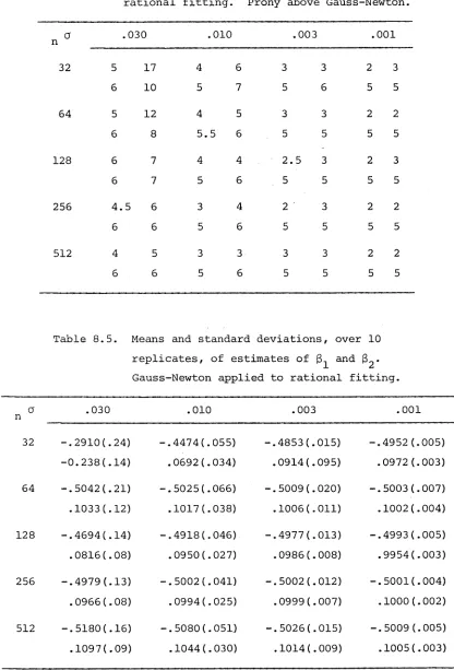
8.3.2 Rational Fitting 132
8.4 Discussion 134
8.4.1 Prony convergence criterion 134
8.4.2 Unmodified Gauss-Newton 134
This thesis deals with algorithms to fit certain statistical models. We are concerned with the interplay between the numerical properties of the algorithm and the statistical properties of the model fitted. The author sees this work as being in the spirit of the papers of Neider and Wedderburn (1972) and Jennrich (1969).
In their influential paper, Neider and Wedderburn introduced the notion of a generalized linear model. They showed how the method of scoring, and its interpretation as a series of linear regressions, provides a unified treatment of the likelihood calculations.
Generalized linear models suppose a distribution which is an
exponential family plus a scale or dispersion parameter, and a linear predictor for a function of the mean of that distribution. In chapters
2 and 3 we propose an extension of generalized linear models by including a linear predictor for (a function of) the dispersion parameter also. We show that the resulting model may be fitted and analysed by fitting two simpler models in turn. The case of the normal distribution is examined in detail.
Similar ideas extend to certain dependent and multivariate models which are dealt with in chapter 4. Chapters 2, 3 and 4 comprise part I of this thesis.
We restrict our attention to separable regressions which satisfy exactly a homogeneous difference equation. For these regressions we can reparameterize in terms of the coefficients of the difference equation, and solve the normal equations using the algorithm of
Osborne (1975). Under similar conditions to those of Jennrich (1969) we prove the asymptotic stability of the algorithm. The major
emphasis is on the case of exponential fitting. Chapters 5 to 8 comprise part II.
In chapter 1 we outline some results, concerning the construction of tests and the convergence of algorithms, based on quadratic
C H A P T E R 1
I NT R O D U C T I O N
1.1 O u t l i n e
In this chapter we outline some basic likelihood theory. Quadratic approximation to the likelihood surface leads to large
sample statistical tests and to the scoring algorithm. In the case of fitting a mean to normal data, or solving a least squares problem, we specialize to the Gauss-Newton algorithm. Generalized linear models are developed as a family of likelihoods for which the scoring
iteration takes the Gauss-Newton form. Sufficient conditions for local convergence of the scoring and Gauss-Newton algorithms are related to Efron's (1975) and Bates and Watts' (1980) measures of curvature. Partitioning the parameter vector leads on the one hand to tests of composite hypotheses, and on the other to modification of the scoring algorithm and to separable regression and coupled iterations in particular. Finally we outline Jennrich's (1969) proof of the asymptotic stability of the Gauss-Newton algorithm.
1.2 A w o r d on n o t a t i o n
Mention needs to be made of several idiosyncratic notations. Firstly vector differentiation and multiplication of tensors. If i
is a scalar function of 0 e , then differentiation produces tensors
y (0) £ lRn is a vector function of 0 , then
and
f3yil
130
jJ
Ü
Cs2 ( 3 y . ^
30. 30, 3 k;
are two and three dimensional tensors respectively. We follow the common (but not entirely consistent: differentiation now produces a row vector!) convention of identifying y with a n X p matrix. No such representation can be made for y , but we will include it also in matrix expressions whenever it is clear which faces act on which. Thus, if y e 3Rn and v e , we will write
••T y y
n 3vl
30. 30, yi 1=1 2 k
P
j/k=l for a p x p matrix,
T •• v y v
r, 2
P 3 Pi
.
I
30. 30. v j vk, .3,k=l
j
k 'i=lfor an n-vector, and even
T •• T v y y v
n p 2 2
3 y.
30. 30 Vj Vk yi i=l j ,k=l 2 k
which is a scalar.
Secondly, scalar functions are taken to operate pointwise on x .
n x i
represents the vector of componentwise products.
If x e 3Rn then ( x ) represents the diagonal matrix with the x. as diagonal elements. The symbols 3E and D are used for expectation and variance or dispersion respectively. Finally if X is a matrix then R(X) is the linear space spanned by its columns.
1.3 T h e L i k e l i h o o d f u n c t i o n
Let &(0) be a log-likelihood function of vector parameter 0 e 0 c ir^3 and (suppressed in our notation) data vector y e 3Rn . Write £,(0) for the efficient score vector, ’£(0) for the observed
information, and 1(0) = IE ( — 56(0) ) = ID (£(0)) for the observed
~ 0 ~ 0 ~
information matrix, the expectation being taken at the same value of 0 as used to evaluate
Z
andZ .
We will generally assume conditions under which the maximum A
likelihood estimate 0 is consistent, a form of the Central Limit Theorem can be applied to n 2
Z
, and a form of the Law of Large Numbers can be applied to ^Z
. We will assume thatI
isnonsingular and is a good approximation to
Z
for 0 near the true value 0q .Throughout this thesis we use methods based on
I
rather than-Z
because it is the exact covariance matrix ofZ
and hencenon-negative definite, and because it is algebraically simpler in the cases we consider. But see Efron and Hinkley (1978).
1.4 L a r g e s a m p l e tests
The approximate normality of
Z
gives us immediately thatwhere ( 7 ) 7 = I . This is the test statistic of the hypothesis 0 = 0 ^ , proposed by Rao (1947).
Expanding Z in a linear Taylor series about 0^ , and approximating -&(0 ) by I (0 ) , gives
(1.2) e -0Q = i<0o) -1
ue0)
and hence
(1. 3) I <®0)lST < ! "So* ä M(0' I) •
This is the Wald test statistic, proposed by Wald (1943).
Expanding Z in a quadratic Taylor series about 0 , and •• /\
approximating -£(0) by I (0 ) , gives
(1 • 4) 2 (Ä(0) - ^(0Q) ) = ^ ? 0)(~ " ? 0 ) and hence
2 ( Z ( Q ) - £(0n)) ~ X2 •
~0 p
This is the likelihood ratio test statistic of Neyman and Pearson (1928).
Under standard conditions, all three large sample tests are asymptotically equivalent.
1.5 The scoring algorithm
Let 0 be an approximation to that value of 0 which maximizes Z( Q ) . We may seek to improve that approximation by maximizing the quadratic expansion of Z about 0 . This is the classical
Newton-** k. k
(1.5) ek+1 - ek = I(0k) 1 ^(0k)
which defines an iteration of the scoring algorithm, usually
attributed to Fisher (1925) . If the process converges then repeated
• A
iteration yields a stationary point which satisfies &(0) = 0 , which
we take to be the maximum likelihood estimate.
Note the similarity between (1.2) and (1.5). In fact the score
A
test is equal to the Wald test with 0 replaced by the value obtained
after one scoring iteration from 0^ . One scoring iteration from a
consistent estimator produces an estimator which may be asymptotically
efficient even if the maximum likelihood estimate is not, and is
equivalent to it if it is. (Le Cam (1956); Bickel (1975) proved
similar results for one-step Huber estimators.)
1.6 Least squares and Gauss-Newton
Suppose the data is normal with mean vector y , a function of
(3 £ JR^ , and covariance matrix VG^ known up to the multiplier G^ .
Then
(1.6) SL = - h log I V O 2 I - h c T 2 (y - y (3) )TV _ 1 (y-y($) )
so
-2•T -1
= a y v (y - y)
-2•T -1* -2-T -1
= -a
y v y +
ay v (y -y)
and
-2-T -1*
1^ = 0 y v y .
2The value of o does not affect the scoring iteration for ß , which
is
In this case the scoring iteration is known as the Gauss-Newton
algorithm. In the simplest case y is linear in (3 and we have
weighted linear regression. The quadratic approximation to i is then exact, 1 + Z = 0 , and Gauss-Newton converges in one step from any starting point.
Maximizing the log-likelihood (1.6) with respect to 3 is equivalent to minimizing the sum of squares
<Mß> = (x ~ y (§))Tv~1(x ~ y (§)) •
In fact the algorithm (1.7) depends on the distribution of y only through its first and second moments. It is generally applied to least squares problems when only second moment assumptions are made. Indeed it is formally available whenever the objective function can be written as a sum of squares. To minimize
f(ß)T f(3)
the algorithm takes the form
(1.8) 3k+1 _ 3k = (fTf) 1 fTf .
This process may perform poorly if IE(f) ^ 0 ; the application of Ross (1982) suffers from this defect.
1.7 G a u s s - N e w t o n and g e n e r a l i z e d l i n e a r m o d e l s
If we allow that the weight matrix V may depend on 3 , the most general objective functions fc(3) for which the scoring iteration takes the form (1.7) are those for which
These are quasi-likelihoods of Wedderburn (1974) and McCullagh (1983) .
If k is a log-likelihood it must have the form
d.9) g_2^ T^ (§ ) }} + c ( ^'a)
for suitably chosen functions b and c , and for V a
transformation of y . In fact it must be that
IE(y) = y(3) = b(V)
and
3D(y) = ö2 V(3) = Ö2 b(V) .
Now let us restrict the y^ to be independent, and to have
densities of the same form except for possibly different values of
and known weights w_^ . Then the log-likelihood (1.9) becomes
(1.10) 0 2 2 {w.(y.V. -b(V.)) +c(y., w.G 2) } i l l l l l
l
where b and c now take scalar arguments. Let us further assume
that the dependence of y on (3 takes the form
(1.11) g(v0 = x3
where X is an n x p matrix and g a scalar function operating
pointwise on y . Then (1.10) and (1.11) define Neider and
Wedderburn's (1972) generalized linear models. The vector X$ is
2
known as the linear predictor, g as the link function and ö as
the dispersion parameter.
The matrix V is now diagonal, and equal to (v(y) “'"w ) with
v(y) = b(v) . And from (1.11) we see that y = (g(y) ) . For
generalized linear models the scoring iteration is therefore
3k+1 - ßk = (XT< g"2v_1w> X)_ 1 XT< g_1v-1w) (y - y)
with the right hand side evaluated at 3 * A little rearrangement
puts (1.12) in the form of a linear regression estimate
(1.13)
with
and
.k+1 T - It
(X WX) X W z
( g ^w )
z = ( g > (y - y) + g (y) .
Iterations of the form (1.13) are often called iteratively
reweighted least squares. The relationship between reweighted least
squares, Gauss-Newton and maximum likelihood estimation is further
discussed by Jorgenson (1983) and Green (1984). McCullagh and Neider
(1983) is a recent monograph on generalized linear models; see also
the review by Pregibon (1984). Fahrmeir and Kaufmann (1985) prove the
consistency and asymptotic normality of maximum likelihood estimates
for generalized linear models. Existence and uniqueness results are
collected by Wedderburn (1976).
In practice Gauss-Newton is applied with line searches or trust
regions to secure convergence; commonly this is accomplished by the
Levenberg-Marquardt modification (Fletcher, 1980). A similar
modification for generalized linear models has been described by
Osborne (1985).
1.8 C o n v e r g e n c e
Consider the iterative process defined by
k+1
x F(xk ) .
*
converges to x from any starting point in some neighbourhood of
* *
x . In that case the process is said to be stable at x . A sufficient condition for stability is given by Ostrowski's Theorem
(Ortega and Rheinboldt, 1970), namely that F is (Frechet) ■k
differentiable at x and that
.
*R = p (F (x ) ) < 1 . *
where p(*) is spectral radius. We call F(x ) the convergence matrix, and R the convergence factor, since if R > 0 then
k+1 * k * f
convergence is linear and ultimately IIx - x II/ II x - x II = R . If R is achieved by a positive eigenvalue of F then convergence is ultimately monotonic, if by a negative eigenvalue then convergence is ultimately oscillatory.
/s
Differentiation of (1.5) at 0 gives the convergence matrix of the scoring algorithm
(1.14) G = r 1 (‘£ + 1) .
This specializes to
(1.15) g = (yTii)~1 yT (y - y)
for Gauss-Newton with identity weight matrix.
Note that (1.14) has Rayleigh quotient
T •• z £z
If £ is negative definite, as it should be at a maximum of £ , then the quotient is less than one for all z . Therefore if the scoring
algorithm diverges from close to a maximum, it is likely to do so in an oscillatory manner.
Consider a reparameterization with Jacobian J . Then I transforms to JTlJ and £,(0) to J(0)T £(0) J(0) . Hence (1.14) transforms to
J_1 I_ 1 Ü + 1) J
to which it is similar. The spectral radius of (1.14) then is a geometric invariant; it does not depend on the parameterization.
If the Gauss-Newton algorithm is actually implemented in a modified form its convergence matrix will be more complicated than
(1.15). The behaviour of the unmodified algorithm though, will be relevant sufficiently close to a solution.
1.9 C u r v a t u r e
1.9.1 Normal c u r v a t u r e
The eigenvalues of (1.14) and (1.15) may be given useful
geometric interpretations. In this section and the next we restrict our attention to (1.15), and return to (1.14) in §1.9.3. In fact
(1.15) is similar to the symmetric matrix
• T* —h ..T • T* —%T b = (vi y) y (y - y) (y y)
which is the "effective residual curvature matrix" of Hamilton, Watts and Bates (1982). Before exploring this further we discuss the
curvatures of one-dimensional curves. Unless otherwise indicated, y /\
and its derivatives are always evaluated at 0 .
Let f be a function mapping 3R into IRn . The range of then defines a one-dimensional curve in n-space. Consider the
l
H
limiting circle through the points f(a-£) , f (a) and f(a + £) as £ "► 0 . The normal curvature at a may be defined to be the inverse radius of this limiting circle, and can be calculated as
"V"
fT f
where is the projection onto N = R (f (ot) ) ^ (Johansen, 1984, pp.80-81).
Now consider one-dimensional curves on the solution locus
{y (0) : 0 e 0} . Corresponding to any direction v e IR^ , there is a line 0 (ot) = 0 + av from 0 in the parameter space, and a lifted one dimensional curve on the solution locus defined by y(0(a)) . We have that
and
dy da yv
T.. v yv .
T
Furthermore the projection of v yv onto R(yv) is the same as its projection onto R(y) . So the normal curvature of the lifted curve is
llvTp yv II
(1.16) K(v) =
v y yv
where P is now the projection onto R(y) • (In the terminology of N
differential geometry, P^U is the second fundamental form of the •
T-surface y(0) , the information matrix y y being the first (Reed, 1975, Johansen, 1984).)
with the solution locus, that is as a normal out. That approach would
exhibit k as a function of the tangent direction yv . As a function
of yv , K is a geometric invariant.
Now return to (1.15). The eigenvalues of G are the stationary
values of the Rayleigh quotient
T-T
V y (y -y) V
( 1 *17) q ( v ) = •
v y yv
Let e = (y - y)/lly - yII , and let be the projection onto R(e) .
Then
q (v) =
llvTP yvll
~ e ~
T-T-v y yT-T-v
Let < ... < A^ be the eigenvalues of G with eigenvectors
x.,...,x . We see that X ./a is the normal curvature at a = 0 of
~1 ~P i
/\ •
the curve y(Q + c o O imbedded in the space spanned by y and e .
A A
We call the X . /cj the normal curvatures of the solution locus at 0
l
relative to e .
Hamilton, Watts and Bates (1982) showed that the A_^ may be used
to give the relative lengths of the axes of ellipsoidal likelihood or
confidence regions. In particular, for likelihood regions, the
relative lengths are \> , . . . ,v with V. = ( 1 - A . ) 2 .
1 p l l
1.9.2 Bates and W a t t s i n t r i n s i c c u r v a t u r e
The quantity (1.16) is the intrinsic curvature, in the direction
associated with v , of Bates and Watts (1980). For the purposes of
calibration, Bates and Watts (1980) define the relative intrinsic
Y(v) = dp\(v) .
We now discuss the relationship between intrinsic curvature and the normal curvatures.
Consider the variability of (1.17) over data sets giving rise to
A A
the same least squares estimate 0 . If we assume 0 to be the true /\
value, the conditional distribution of y-y(0) given
U (0)T (y - y (9)) = 0 is W(0,O2P ) . Under this distribution
~ ~ ~ N
llvTP 11 v II2
2 ~ N ~ -1
EJ |§ (v)) = 0 — tT^:— j = p Y(~} *
Y ~ (v y yv)
In any particular direction then, p ^(v) gives the standard deviation of the Rayleigh quotient q(v) , conditional on the least squares estimate being at the point of evaluation. It may be viewed as a before-the-data estimate of the size of the Gauss-Newton
convergence matrix in that direction and at that point.
Bates and Watts (1980) define their summary measures of intrinsic 2
curvature by maximizing or averaging Y (v) over v . Thus
r2 = max Y2 (y) v
and
2 _ 2, .
Y = E Y v
'RMS v ' ~
• T* -1
the expectation being taken over v ~ W(0,(y y) ) . The second 2
measure, Y ^ g is f°ur times the measure of nonlinearity, , derived by Beale (1960). It can be calculated explicitly as follows. Let be the t'th p x p face of (y y) 2P^y(y y) 2
d = (y y) 2 v . Then (1.16) becomes
2 (dTA d)2 K2 (d) =
(dTai
2
Taking expectation over d ~ W(0,I) , and using the independence of
T
3 t
— —— and d d to carry the expectation through to numerator and d a
denominator,
^2 'RMS pö
Z 3EJ (dTA d ) 2 d ~ t~ t
T 2 3E, (d d)
d ~ ~
M 2 n , + i s v , ) 2}
t i t - 1 i t ' 1
„ 2
2 p + P
where X ,.
L. / X
.,X are the eigenvalues of A ,
t , p t
2 {2IIA 1 1 + (tr A r }
t t F t
P ( P + 2)
where 11*11 is Frobenius norm and tr (•) is trace. F
Both summary measures inherit geometric invariance from K(v) :
2 ^2
r is obtained by maximizing pO K(v) over tangent directions yv ;
2
Yr^S is obtained by averaging over yv symmetrically distributed in
the tangent plant R(y) .
2 2
Both T and provide useful bounds for the expected size
of the convergence factor. In fact, since
2 2
max IE (q (v) ) < IE (max q (v) )
we have immediately that
1 2 „ 1 „
p Y RMS “ p r “ ^ y l e (P (G)) .
We view
T
itself as a conservative (large) estimate of2 2 -1
3Ey |g (p (G)) . Comparing
Y
with F(p; n-p; .95) as do Bates andconservative indeed from the point of view of convergence,
We can also show that
(1.18)
1 2
p ^RMS
23Ey I 6 (llGllF )+3Ev [ e (tr G )2 , 1
p(p + 2) ä p E y |0 (llGllF> •
The equality of (1.18) is established as follows. Since
/s 2
(y -y) ~ N(0,O P^) , ( y - y ) can be written as with
e ~ W(0,Q I) . Then G has the same eigenvalues as S e a
t Therefore
and
(1-19)
IE (tr G) = o 2 tr A
y|0 t 1
3E I S (IIGII2) = a2 2 IIA II2
y I Ü F t F
-2 2
T he inequality of (1.18) follows from the fact that IIGII (tr G)
F
achieves its maximum of p when all the eigenvalues of G are equal.
Alternatively we could bound the expected square of the
2
convergence factor using = IE |g (IlGlI^) itself, by
- S' < IE (p2 (G) ) < S .
p 2 y|0 2
Higher moments may be bounded similarly. For example
S = IE i g tr(G4 ) = 3Q4 { 2 tr(A4 ) + 2 2 tr (A2 A 2 )}
4 y 10 t _ s t
s<t and
i S 4 S E y | 0 (p4<G)) £ S4 •
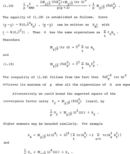
We conclude this section with a table extracted from table 1 of
t 2
Hamilton, Watts and Bates (1982). The table shows that T is
Table 1 of Hamilton, Watts and Bates (1982) and Table 2 of Bates
[image:26.569.82.499.150.645.2]Table 1. Maximum relative intrinsic curvature, minimum and maximum eigenvalues of the convergence matrix and the convergence factor for 18 data sets.
Data Set r X1 (G) A (G)
P P (G)
1 .03 -.00 .00 .00
2 .06 -.00 .00 .00
3 .08 -.17 .00 .17
4 .07 -.10 .00 .10
5 .21 -.00 .10 .10
9 .18 1 >x>0 .02 .06
13 .01 -.00 .00 .00
14 .15 -.00 .08 .08
15 .04 -.04 .00 .04
16 .04 -.00 .02 .02
17 .25 1 0 o .15 .15
18 .00 -.00 .00 .00
19 .02 -.02 .00 .02
20 .02 -.06 .00 .06
21 .90 1 O KD .26 .26
22 .08 -.19 .00 .19
23 .09 -.02 .10 .10
24 .37 -.04 .10 .10
2
credible as a conservative estimate of IE (p (G)) , and that p(G) is well within the bounds for a point of attraction for all 18 data sets.
For each of Bates and Watts' measures of intrinsic curvature there is a corresponding measure of parameter effects curvature which depends on the parametrization (Bates and Watts 1980, 1981; Kass, 1984). We have neglected these because p(G) is a geometric
[image:27.569.151.480.143.565.2]invariant. Fortran routines to calculate Bates and Watts' summary measures of curvature are given in Bates, Hamilton and Watts (1983).
1.9 . 3 Efron c u r v a t u r e
In our discussion of curvature so far we have restricted
ourselves to least squares problems and to particular directions in the parameter space. In the general case we consider the variability
2
of (1.14) conditional on Z . The covariances of the p elements of the matrix G form a four-dimensional tensor
no ,, (I-1Ci + I)) = (y. . )
y|£ 1 3,mn
which holds all the second moment information about G . This is the multiparameter counterpart of Efron's (1975) stati-sti-cal curvature.
Let
Then
where (I^) = I
Cov (Z. .,Z 1&) = a . . 13 m n1 13 ,mn
2 v- _.ki r Zn Y, . . = 2, I I a. .
'k3,m& . 1 3,mn xn
Dividing again by I gives
Bk£ 2 Ykj,m£ 1 3m
jm
-2
which is the order n correction to the covariance matrix of the maximum likelihood estimate due to statistical curvature. See Reeds
(1975), Madsen (1979), Amari (1982).
Bounds for the expected squared convergence rate may be had from
E y | l l,G,F ) S y ii/jj
Specializing to least squares gives
Y
m i , £n2
st 2
jk
• T* mj .. (y y) y
s, ij t,k£
* T * k n (y y)
and (1.20) becomes (1.19).
Efron's statistical curvature is also discussed by Efron (1978)
and Efron and Hinkley (1978).
. 1 . 1 0 T e s t s of C o m p o s i t e H y p o t h e s e s
P 2 P 2
Suppose that 0 is partitioned into 0^ e 3R and 0^ e JR ,
p^ + p ^ = P , and that
and
T =
are conformal partitions of £ and
this and the next two sections of the
I
. Frequent use will be made in Tblock L D L decomposition
(1.21)
I
T
o
H
v
_____
__
o
r—
1 fl IL1 L 12I I
i h l h 1 * L 0 I - I 2 2 1 1 I 1 I1 2 ^ r— o
H
V
This decomposition suggests the transformation to orthogonal
parameters
f a . + i . .fl ^ r0
(1.22) L 0 = .1 i 12.2
1§2
= ~1.2
>?2 '
(1.23) L H
£ -I I X£ ,
v 2 21 1 1" 2.1
and information matrix
(1.24) L 1
I
l"I
0
I
o
T 1 1
o
i -i
r h^ 7 7 1 1 1 7 J •° £
i-Suppose that we wish to test 0^ = Ö^q , and the 0^ enter as unknown nuisance parameters. Locally all the information about 0^
. . f
and 0^ is contained in £^ and £^ • So we form the conditional distribution of £^ given £_^
£ I L ~ W(I , I )
2 1 1 21 1 1' 2.1
and obtain the statistic
(1.25)
l t \ *2.1 ~ W(°'I)
based on £ but corrected for regression on £ .
^ _L
It remains to replace 0^ with an estimate in (1.25). It is A
usual to use ' t*ie va-*-ue which maximizes £ with 0^ fixed at 0 . Then (1.25) becomes
(1.26)
°20> ä W(°'I)
which is Rao's (1948) score test for composite hypotheses. Note that
A • • 0
at 0^ = ' ^2 1 = ^2 s^nce £-^ = 0 . A statistic equivalent
to (1.26) was independently derived by Aitchison and Silvey (1958, 1960), and has become entrenched in the econometrics literature as the Lagrange rmlt-iplier test. See the review of Breusch and Pagan (1980) . t
Note that estimates need to be obtained under the null hypothesis only.
If some other estimate of 0^ is used, then (1.25) is the C(a)
test proposed by Neyman (1959) (extended to multi-parameter hypotheses
by Buhler and Puri (1966); see also Moran (1970)). Neyman's
contribution was to show that the asymptotic properties of (1.25) are
retained for any estimator which is "root-n consistent", that is for
ki a .
which n |0 ^ — ® i o ‘ remaans bounded in probability.
Partitioning (1.2) gives
(1.27)
I
1i
L
2.1 *2.1which with (1.25) gives
( 1 - 28> h i A ' V £ w ( 0 ' I)
which is the Wald test of a composite hypothesis. It is usual to use
0^ for 0^ in (1.28) so that only unrestricted estimates are
required.
Note that if -^2 is chosen to be the block Choleski factor
(1.29) r^2
then (1.26) and (1.28) are simply the conformal components of (1.1)
and (1.3).
We can decompose (1.4) also as
- Ä(?10'?20) } + 2 U ( ? 1 ^ 2 ) (1.30)
(~1.2 ?1 0.20} *1(~1.2 §1 0.20) + (~2 ?20} *2.1 (~2 §20) '
(1.30) as the terms conditional on establishes
( 1 . 3 D
2U ( e 1 .e2 ) - a ( e l ( e 2 0 ) . e 2 0 )} S (§2
- g 2 0 ) 5
This is the likelihood ratio test statistic for the composite /\
hypothesis. Note that both restricted (0^(0 )) and unrestricted
A / \
(0 /02) estimates are required.
A
The above treatment in terms of a partition of 0 implies the
form of the test statistics for general composite hypotheses specified
in terms of restrictions. Suppose we wish to test that h(0) = 0 ,
where h is a r-dimensional function of 0 . If h has full rank
T T T
then we define a reparametrization of 0 to (f) , with (J) = (4>^, (j)^) and (j) = h , and test cj)^ = 0
1.11 N e s t e d a n d C o u p l e d I t e r a t i o n s
Suppose that 0 is partitioned as in §1.10. Using the
decomposition (1.21) of
I
we may write the scoring iteration (1.4)as
(1.32)
0k+1 - 0k
~1 ~1
0k+1 - 0k
F (0k , 0k ) 1 - 1' ~ 2;
~2}
*1 Ä1 *1 I12I2.1^2.1 7 1 £
Z . 1 2.1
We may describe (1.32) as parallel 'iterations for 0^ and 0^ .
An attempt to accelerate the convergence of (1.32) is to apply
the (nonlinear) Gauss-Seidel principle that information be used as
soon as it is available. Using the already updated 0^ to update 0^
gives
st-sJ ■
v»5- s
5
>
which we call alternate iterations. It is worth noting the special
case with I = 0 , for which the alternate iterations are
(1.34)
h 1 V &
h 1 y s T 1
We consider two other algorithms which attempt to further
separate the iterations for
0i and ~ 2 ■ Let 0 l(02 ) be the value
of 0^ which maximizes Z with
§2 fixed. We define nested
iterations to be the process
(1-35)
,k+l /v k
®lf02>
®2+1 '■§2 ■
v?r
“ l2 (0l+ 1 'C
D
? /
Note that for
ef
1 so defined, Z ^ = Z2 since = 0 Comparewith (1.26).
/\
I
f
h
(§2) is available in closed form, the 0^ areoften said to be separable.
Similarly let 0^(©i) maximize Z for fixed 0^ . We define
coupled iterations to be the process
(1.36)
®1+1 = ? l (§2)
,k+l
®2(ä +1)
Both nested and coupled iterations can be viewed as a reduction in the
dimension of the fitting problem, since we can summarize (1.35) as
(1'37> §2+1 = §2 + I2!l V ® 1 (®2>' ®2> and (1.36) as
/\ V_L_ 1 /\ /\
without involving ©^ .
Coupled iterations consist of iterating each equation of (1.34) to convergence before alternating to the other equation. If 0^ and
are orthogonal then the process is a variation of alternate
iterations. We can relate nested to alternate iterations through the transformation (1.22). The alternate iteration for the derived
orthogonal parameters is
(1.39)
flk+1 ftk §1.2 ' §1.2
§2+1 - §2
i
1
jpe*, e*)
h ! i V X " 1 ' §2>
Nested iterations consist of iterating the first equation of (1.39) to convergence before alternating to the second equation. If it happens that = ®i + ^i"*" ^°r ' aS aS tke case f°r
linear parameters in least squares, then nested iterations for 0^ and are exactly equivalent to alternate iterations for 0^ ^ and
§2 •
Another useful description of nested iterations, although one which characterizes I ^ as only one of several possible
approximations to the Hessian, is the following. Minimize with respect to ©2 the reduced objective function
^ (e2) = ' §2}
which is not now a likelihood function. We find, as did Richards (1961), that
* ■ V § 1 (§2>' §2> and
where
'z
=Z , - Z , ' Z
1Z
. We apply Newton-Raphson to minimize • -1- ^ -L -1 -1 “i[i and approximate -£ ^ with ^ •
Coupled iterations may be identified as a nonlinear Gauss-Seidel iteration to solve the partitioned Z = 0 (Ortega and Rheinboldt, 1970). We will refer to the calculation of anc^ ^2^1^ aS fitting submodels corresponding to the subvectors 0^ and 0^
respectively. The terminology is justified by observing that if one subvector is fixed,
Z(Q
, 0^) may be considered a log-likelihood function of the other subvector alone, possibly in terms of derived data calculated from the original data and the fixed parameters. If 0^ and are orthogonal, then the scoring iteration for 0 may be interpreted as comprising an iteration for 0^ and an iteration for© 2 , each in their own submodels.
Note the similarity of (1.27) and (1.35). The score test (1.26) for composite hypotheses is equivalent to the Wald test (1.28) but
— • /\ /\
with one nested iteration ®20 + ^2 1 ^ 2 ^ 1 ^ 2 0 ^ ' ^20^ an P^ace *
1.12 C o n v e r g e n c e R a t e s of P a r t i t i o n e d A l g o r i t h m s
1.12.1 N e s t e d i t e r a t i o n s
We show that nested iterations have a convergence factor less than or equal to that of the full scoring iteration. Differentiating
(1.37) at 0_ , and using (0*J = i"*” ^ n / gives the
~2 dt^ ^
convergence matrix for nested iterations
(1‘40) G “ I + I 2 U *2.1 ’
We show that the spectral radius of (1.40) is less than that of (1.14) by showing that the extreme eigenvalues of ^ 2 1 ^2 1 are bounded ky
Let P be the p x matrix (01) . We observe that
-1 T -1 --1 T--1
1
2 ^ = P I P and ^ 2 1 = ? ^ P * Therefore_ i t — X T*-—1 — 1
X 2 ^ 2 1 = P ^ P(P
Z
P) , which has Rayleigh quotient(1.41)
T Tt-1 z P I Pz
T T-- —1 z P
Z
Pzfor z £ IR extrema of
or of
(1.42)
The extrema of (1.41) are equivalent to constrained
T - i
v
I v
Ty-1
V
Z
VT** v
Zv
Tt
V Iv
over v e 3R^ , and hence are bounded by the unconstrained extrema.
-1*.
Observing that (1.42) is the Rayleigh quotient
of
I
Z
completes the demonstration.1 . 1 2 . 2 C o u p l e d i t e r a t i o n s
The convergence matrix for coupled iterations emerges, from differentiating (1.38) at 0 , as
(1.43) G = i,1 «,
since
dex W = —
ö
0 and
--2 --21 d0.
spy “
- W 2
IfZ
isnegative definite, as it will be at a maximum of
Z
, then the eigen values of G all lie between 0 and 1 ; they may be recognized as the canonical correlations (e.g. Rao, 1973, §8f.l) calculated from the partitioned covarance matrix-JL - L
This shows that any maxima is a point of attraction for coupled
iterations; furthermore the convergence is monotonic.
On the other hand, for G to tend to zero for increasing sample
sizes, it is necessary that I = IE (-£, ) = 0 , that is that 0^
and 0^ be orthogonal. if this is not the case, then coupled
iterations will be the slowest of the algorithms considered in §1.11
for sufficiently large samples.
1.13 Separable Regression
The most common application of nested iterations is to nonlinear
regression. Consider the least squares problem with parameters
T T T
0 = (a , 3 ) and with
(1-44) 0(a, 3) = ( y - p ) T ( y - p ) .
Suppose the mean ji has the functional form
y
2 x . . ( 3 ) al i ~
i = 1,... ,n
with each x . . a ID
parameters and the
matrix function X
smooth function of ß • The a
3j nonlinear. Gathering the
allows us to write
are linear
x. . into the iD
y = x(3)a .
We assume X to be of the full rank, at least in a neighbourhood of
the true value 3q •
The parameters a_. are separable since
(1.45)
a(3) = (xTx)_1
XT y .Substituting (1.45) back into (1.44) gives
4K3) = <M§(3) , 3) = yT(i - P x)y
with P = X(X X) X the projection onto R(X) . Also X
T . - I T
I2 x (a(3)/ 3) = y^y^, - y^x(xTx) V y ^ 2.1 ~ ~
(1.47)
application of nested iterations to the least squares problem gives
(1.48) 3 k+1 -3 = ( y ^ d - P ^ y ^ ) k *T v* v-1 -Ty^(y-y) •
Separating the linear parameters was suggested by Richards (1961)
in a maximum likelihood setting, and by Ross (1970) and Lawton and
Sylvestre (1971) for regression. Richards suggested Newton-Raphson to
minimize ijj(ß) , while Lawton and Sylvestre suggested finite
difference methods. Golub and Pereyra (1973, 1974) applied the formal
Gauss-Newton algorithm (1.8) to ijj(ß) with f = ( I - P )y , and named
the result the variable projection algorithm. Kaufman (1975) derived
our nested iteration using differentiation of orthogonal matrices.
Ruhe and Wedin (1980) showed that the variable projection algorithm
and nested iterations have similar convergence factors, and both
factors are bounded by that of Gauss-Newton on the unseparated problem.
In fact, the eigenvalues of the convergence matrix for the variable
projection algorithm are the normal curvatures of the solution locus
(multiplied by O ) , restricted to the sublocus determined by
a = a(3) •
Each nested iteration requires the same amount of computation as
does an iteration of unseparated Gauss-Newton, as can be seen from our
derivation in §1.11. Golub and Pereyra (1973) and Ruhe and Wedin
(1980) both found that iterations of the variable projection algorithm
1.14 T e s t s in S u b m o d e l s
Our aim in this section is to make an observation about
orthogonal parameters and to develop the concept of a submodel a
little further. Suppose that
0
is partitioned into orthogonalsubvectors 0 and y , and that these in turn are partitioned into
/ 02 and Y , Y . The dimensions are p , p 2 and q 1 , q 2
say. Suppose that we wish to test 02 = 0 and Y 2 = y . Then
the score test statistic of this combined hypothesis simply consists
of the statistics for the hypothesis 02 = 0 ^ and y = y tested
separately. The same is true of the Wald test, but not of the
likelihood ratio test.
Let conformal partitions of & and I be
'o
0
.and
Y'
[h
Z 01 12
X 0 X 0
21 2
I
h Y
I
i—
i
C
M
>
-Y 12 2
We find the score test (1.26) of 02 = ß and Y 2 = y ^ is
iT
2
y
2.1 P2
f h l Y2.1 L
-Jg
in an obvious notation. Here J r , & n is the score test of
02.1
32 = 320 in the B-submodel with y fixed at ' ~20^ *
Similarly
I 2
Z
is the test of = y ^ in the y-submodel with\ l Y 2 ~2 '2° '
3 fixed at §20^ ’ In itS ^ form
(1.50)
H i
1
L + £T
i
1
i
^2 ß2.1 132 Y 2 Y2.1 Y 2 P2+q2
the score test emerges as the sum of the statistics from the submodels.
The same observation is true for the Wald test, with
(1.51)
7B2 x (?2 ~20}
XB2 1 (^2 ~20}
W(0,I)
and
( 1 * 5 2 ) (§2 ?20}
\
x (?2 ~20) + ($2 ~20} \ 2%
2 0}
~ X P2+q2Here (1.51) consists of the Wald test of 3 = 32q in the 3-submodel with y fixed at y , and the Wald test of Y2 = y in the
A y-submodel with 3 fixed at 3 .
The likelihood ratio test of the combined hypothesis cannot be expressed exactly as the sum of statistics from submodels. This is a consequence of the fact that both restricted and unrestricted
estimates of the nuisance parameters are required. An attempted
decomposition would take the form of (1.30): the first term is a test in a submodel, but the second is not.
1 .15 A s y m p t o t i c S t a b i l i t y of the G a u s s - N e w t o n I t e r a t i o n
We do so in some detail because it foreshadows a proof of the stability of the Prony algorithm in chapter 7 under very similar assumptions.
Define the matrix function of 0
(1.52) Gn (0) = Cy(0)T yC0)) 1 y(0)T (y-]4(0)) .
At 0 , G is the convergence matrix (1.15) of the Gauss-Newton algorithm. In summary, we prove that Gr(0) tends to zero by proving
/\ t* ~
that n y (0) y(0) tends to a nonsingular matrix while
—1 . . ^ T /s
n y (0) (y-y(0)) tends to zero. Before we can be more precise we need to be more specific about our assumptions. Assume that
(a) Error structure. The y - y (0q) are independently and
2
identically distributed with mean zero and variance 0 ; 0^ is an interior point of the compact set 0 c IR^ .
(b) Unique mini-mum. The function
Q(0) = lim - (y (0) - y (0 ) ) T (y (0) -y(0n))
~ n ~ ~ ~U ~ ~ ~ ~U
n - K »
has a unique minimum over 0 at 0 .
1 T
(c) Smoothness of y . All limits of the form lim — f g with
9 92 n~*C ° n
f,g = y , t~ ~ , exist and are continuous on 0 .
~ ~ ~ 0 0 . 0 0 . 0 0 .
1 1 3
(d) Nonsingular information matrix. The matrix A defined by
i 3yT A ij = lim n 90~ 90~
n-x» i j
is nonsingular at 0^ .
We need the following form of the Law of Large Numbers.
such that
1 n
n 2
i=l
f. ( 9 J f . (0O) l - l i ~ 2
converges uniformly on 0 x 0 , then
1
n n 2
i=l
f. (6) (y. - y . (0 ))
l l l 0
a.s. -> 0
uniformly on 0 .
Proof.
See Jennrich (1969). □We will accept the consistency of 0 as having been established
(see Jennrich (1969)), and are now in a position to prove
Theorem
2. Under conditions (a) to (d).,G (0) n
-a.s. 0 .
. T .
Proof.
We must establish that exists (i.e. y y is nonsingular)and converges, uniformly in some neighbourhood S of 0^ , to a
continuous function G which is zero at 0^ . Having done so we can
write
IIG (0)11 < IIG (0) - G (0JII + IIG (0 ) - G (0 ) II
n - n - n -0 n -0 -0
where II• II is any matrix norm. We can make G (0) - G (0 ) small by
n - n -0
choosing 0 within a suitably small neighbourhood £ S of 0q ,
and G^(0q) - G ( 0q) s m a H by choosing n large. Finally, using
A A
consistency of 0 , we can choose n large to ensure 0 e a.s.
thus proving the theorem.
The existence and convergence of G is established as follows.
n
on a compact neighbourhood S of 0q . Since n y y A uniformly, •
T-y T-y is nonsingular in S for n sufficientlT-y large. We can write then, for 0 e S ,
Gn (0) = (n vi(ö)t vi(0)j”1 ^ ^ 0 ) T ^ y - y ( e o)) + (H (0o} *
*p ^ g
By the Law of Large Numbers n y(0) (y-y(0 )) ' 0 . Let
F (0) = lim ^ y(0)T (y(0Q) - y (0)) . n-x»
We find that G (0) a '_f’ a (0) ^ F(0) uniformly for 0 e S , and n ~
observe that F is zero at 0^ . n
C o r o l l a r y .
The Gauss-Newton iteration is asymptotically stable.R e m a r k on a s y m p t o t i c a r g u m e n t s
The operational content of an asymptotic argument such as the above is that it leads, at least implicitly, to an expansion for the
/\
quantity of interest, in this case ptG^C©)) , in terms of increasing negative powers of n . This expansion then provides an approximation which is applied in finite samples.
Assumptions (a) to (d) above ensure that the information matrix * T*
y y is of order n . This is a stronger growth condition than necessary. Wu (1981) has shown that, for consistency of 0 , a necessary condition is that
( 1 * 53) Q n (0) = (y (0) - y (0o ) ) T ( y (0) - y ( 0 o )}
for all 0 0q . Condition (1.53) is also sufficient when combined with other assumptions which basically ensure that the minimum
eigen-•
provide more information about constants appearing in the above mentioned expansion.
It is also assumed in the above proof that 0 is restricted to a compact set 0 . In many specific examples it is possible to prove that the unrestricted least squares estimate must eventually belong to a compact set containing 0^ , thus making the prior assumption
unnecessary. This is an important point, because if compactness of 0 was critical, and 0 had to be chosen very large indeed in a specific example, then there would be no reason to expect that constants