Determination of the proton spin structure functions for 0.05 < Q(2)  < 5GeV(2) using CLAS

Q(2) < 5GeV(2) using CLAS

.

White Rose Research Online URL for this paper:

http://eprints.whiterose.ac.uk/136369/

Version: Published Version

Article:

Fersch, R. G., Guler, N., Bosted, P. et al. (152 more authors) (2017) Determination of the

proton spin structure functions for 0.05 < Q(2) < 5GeV(2) using CLAS. Physical Review C.

065208. ISSN 1089-490X

https://doi.org/10.1103/PhysRevC.96.065208

[email protected] https://eprints.whiterose.ac.uk/ Reuse

Items deposited in White Rose Research Online are protected by copyright, with all rights reserved unless indicated otherwise. They may be downloaded and/or printed for private study, or other acts as permitted by national copyright laws. The publisher or other rights holders may allow further reproduction and re-use of the full text version. This is indicated by the licence information on the White Rose Research Online record for the item.

Takedown

If you consider content in White Rose Research Online to be in breach of UK law, please notify us by

Determination of the proton spin structure functions for 0

.

05

<

Q

_<

_{5 GeV}

_{using CLAS}

R. G. Fersch,45,7_{N. Guler,}31,37_{P. Bosted,}39,45_{A. Deur,}39_{K. Griffioen,}45_{C. Keith,}39_{S. E. Kuhn,}31_{R. Minehart,}44_{Y. Prok,}31 K. P. Adhikari,26_{S. Adhikari,}11_{Z. Akbar,}12_{M. J. Amaryan,}31_{S. Anefalos Pereira,}18_{G. Asryan,}46_{H. Avakian,}39,18_{J. Ball,}6

I. Balossino,17N. A. Baltzell,39M. Battaglieri,19I. Bedlinskiy,23A. S. Biselli,9,4W. J. Briscoe,14W. K. Brooks,40,39 S. Bültmann,31V. D. Burkert,39Frank Thanh Cao,8D. S. Carman,39S. Careccia,15,31A. Celentano,19S. Chandavar,30 G. Charles,31_{T. Chetry,}30_{G. Ciullo,}17,10_{L. Clark,}42_{L. Colaneri,}8_{P. L. Cole,}16,39_{N. Compton,}30_{M. Contalbrigo,}17_{O. Cortes,}16

V. Crede,12_{A. D’Angelo,}20,34_{N. Dashyan,}46_{R. De Vita,}19_{E. De Sanctis,}18_{C. Djalali,}36_{G. E. Dodge,}31_{R. Dupre,}22 H. Egiyan,39,45_{A. El Alaoui,}40_{L. El Fassi,}26_{L. Elouadrhiri,}39_{P. Eugenio,}12_{E. Fanchini,}19_{G. Fedotov,}36,35_{A. Filippi,}21

J. A. Fleming,41_{T. A. Forest,}16_{M. Garçon,}6_{G. Gavalian,}39,27_{Y. Ghandilyan,}46_{G. P. Gilfoyle,}33_{K. L. Giovanetti,}24 F. X. Girod,39,6C. Gleason,36E. Golovatch,35R. W. Gothe,36M. Guidal,22L. Guo,11,39K. Hafidi,1H. Hakobyan,40,46

C. Hanretty,39_{N. Harrison,}39_{M. Hattawy,}1_{D. Heddle,}7,39_{K. Hicks,}30_{M. Holtrop,}27_{S. M. Hughes,}41_{Y. Ilieva,}36,14 D. G. Ireland,42_{B. S. Ishkhanov,}35_{E. L. Isupov,}35_{D. Jenkins,}43_{K. Joo,}8_{D. Keller,}44_{G. Khachatryan,}46_{M. Khachatryan,}31 M. Khandaker,28,*_{A. Kim,}8_{W. Kim,}25_{A. Klein,}31_{F. J. Klein,}5_{V. Kubarovsky,}39,32_{V. G. Lagerquist,}31_{L. Lanza,}20_{P. Lenisa,}17

K. Livingston,42_{H. Y. Lu,}36_{B. McKinnon,}42_{C. A. Meyer,}4_{M. Mirazita,}18_{V. Mokeev,}39,35_{R. A. Montgomery,}42 A. Movsisyan,17C. Munoz Camacho,22G. Murdoch,42P. Nadel-Turonski,39S. Niccolai,22G. Niculescu,24I. Niculescu,24 M. Osipenko,19A. I. Ostrovidov,12M. Paolone,38R. Paremuzyan,27K. Park,39,25E. Pasyuk,39,2W. Phelps,11J. Pierce,44,29

S. Pisano,18_{O. Pogorelko,}23_{J. W. Price,}3_{D. Protopopescu,}27,†_{B. A. Raue,}11,39_{M. Ripani,}19_{D. Riser,}8_{A. Rizzo,}20,34 G. Rosner,42_{P. Rossi,}39,18_{P. Roy,}12_{F. Sabatié,}6_{C. Salgado,}28_{R. A. Schumacher,}4_{Y. G. Sharabian,}39_{A. Simonyan,}46 Iu. Skorodumina,36,35_{G. D. Smith,}41_{D. Sokhan,}42_{N. Sparveris,}38_{I. Stankovic,}41_{S. Stepanyan,}39_{I. I. Strakovsky,}14

S. Strauch,36M. Taiuti,13,‡Ye Tian,36B. Torayev,31M. Ungaro,39,32H. Voskanyan,46E. Voutier,22N. K. Walford,5 D. P. Watts,41X. Wei,39L. B. Weinstein,31N. Zachariou,41and J. Zhang39,31

(CLAS Collaboration)

1_{Argonne National Laboratory, Argonne, Illinois 60439, USA}

2_{Arizona State University, Tempe, Arizona 85287-1504, USA}

3_{California State University, Dominguez Hills, Carson, California 90747, USA}

4_{Carnegie Mellon University, Pittsburgh, Pennsylvania 15213, USA}

5_{Catholic University of America, Washington, D.C. 20064, USA}

6_{Irfu/SPhN, CEA, Université Paris-Saclay, 91191 Gif-sur-Yvette, France}

7_{Christopher Newport University, Newport News, Virginia 23606, USA}

8_{University of Connecticut, Storrs, Connecticut 06269, USA}

9_{Fairfield University, Fairfield, Connecticut 06824, USA}

10_{Universita’ di Ferrara, 44121 Ferrara, Italy}

11_{Florida International University, Miami, Florida 33199, USA}

12_{Florida State University, Tallahassee, Florida 32306, USA}

13_{Università di Genova, 16146 Genova, Italy}

14_{The George Washington University, Washington, D.C. 20052, USA}

15_{Georgia College, Milledgeville, Georgia 31061, USA}

16_{Idaho State University, Pocatello, Idaho 83209, USA}

17_{INFN, Sezione di Ferrara, 44100 Ferrara, Italy}

18_{INFN, Laboratori Nazionali di Frascati, 00044 Frascati, Italy}

19_{INFN, Sezione di Genova, 16146 Genova, Italy}

20_{INFN, Sezione di Roma Tor Vergata, 00133 Rome, Italy}

21_{INFN, Sezione di Torino, 10125 Torino, Italy}

22_{Institut de Physique Nucléaire, CNRS/IN2P3 and Université Paris Sud, Orsay, France}

23_{Institute of Theoretical and Experimental Physics, Moscow, 117259, Russia}

24_{James Madison University, Harrisonburg, Virginia 22807, USA}

25_{Kyungpook National University, Daegu 41566, Republic of Korea}

26_{Mississippi State University, Mississippi State, Mississippi 39762-5167, USA}

27_{University of New Hampshire, Durham, New Hampshire 03824-3568, USA}

28_{Norfolk State University, Norfolk, Virginia 23504, USA}

29_{Oak Ridge National Laboratory, Oak Ridge, Tennessee 37830, USA}

30_{Ohio University, Athens, Ohio 45701, USA}

31_{Old Dominion University, Norfolk, Virginia 23529, USA}

32_{Rensselaer Polytechnic Institute, Troy, New York 12180-3590, USA}

33_{University of Richmond, Richmond, Virginia 23173, USA}

34_{Universita’ di Roma Tor Vergata, 00133 Rome, Italy}

36_{University of South Carolina, Columbia, South Carolina 29208, USA}

37_{Spectral Sciences Inc., 01803 Burlinton, Massachusetts, USA}

38_{Temple University, Philadelphia, Pennsylvania 19122, USA}

39_{Thomas Jefferson National Accelerator Facility, Newport News, Virginia 23606, USA}

40_{Universidad Técnica Federico Santa María, Casilla 110-V Valparaíso, Chile}

41_{Edinburgh University, Edinburgh EH9 3JZ, United Kingdom}

42_{University of Glasgow, Glasgow G12 8QQ, United Kingdom}

43_{Virginia Tech, Blacksburg, Virginia 24061-0435, USA}

44_{University of Virginia, Charlottesville, Virginia 22901, USA}

45_{College of William and Mary, Williamsburg, Virginia 23187-8795, USA}

46_{Yerevan Physics Institute, 375036 Yerevan, Armenia}

(Received 20 July 2017; revised manuscript received 16 November 2017; published 27 December 2017)

We present the results of our final analysis of the full data set ofg₁p(Q2_{), the spin structure function of the}

proton, collected using CLAS at Jefferson Laboratory in 2000–2001. Polarized electrons with energies of 1.6, 2.5, 4.2, and 5.7 GeV were scattered from proton targets (15_NH

3dynamically polarized along the beam direction)

and detected with CLAS. From the measured double spin asymmetries, we extracted virtual photon asymmetries

Ap1 andA

p

2 and spin structure functionsg

p

1 andg

p

2 over a wide kinematic range (0.05 GeV 2

< Q2_{<5 GeV}2

and 1.08 GeV< W <3 GeV) and calculated moments ofgp₁. We compare our final results with various theoretical models and expectations, as well as with parametrizations of the world data. Our data, with their precision and dense kinematic coverage, are able to constrain fits of polarized parton distributions, test pQCD predictions for quark polarizations at largex, offer a better understanding of quark-hadron duality, and provide more precise values of higher twist matrix elements in the framework of the operator product expansion.

DOI:10.1103/PhysRevC.96.065208

I. INTRODUCTION

Understanding the structure of the lightest stable baryon, the proton, in terms of its fundamental constituents, quarks and gluons, is a long-standing goal at the intersection of particle and nuclear physics. In particular, the decomposition of the total spin of the nucleon, J ₌1₂, into contributions from quark and gluon helicities and orbital angular momentum still remains an open challenge 30 years after the discovery of the “spin puzzle” by the European Muon Collaboration [1]. Although deep-inelastic electron and muon scattering (DIS), semi-inclusive DIS (SIDIS), proton-proton collisions, deeply virtual Compton scattering (DVCS), and deeply virtual meson production (DVMP) have all been used to understand nucleon spin, inclusive polarized lepton scattering remains the benchmark for the study of longitudinal nucleon spins. The inelastic scattering cross section can be described in the Born approximation (1-photon exchange) by four structure functions (F₁p,F₂p,g₁p, and g₂p), all of which depend only onQ2_{, the 4-momentum transfer squared, andν, the virtual} photon energy. Two of these,g₁p andg₂p, carry fundamental information about the spin-dependent structure of the nucleon. The status of the world data forgp₁ andgp₂ and their theoretical interpretation are reviewed in Refs. [2,3].

The new experimental data from Jefferson Laboratory (JLab) reported in this paper expand significantly the kinematic

*_{Present address: Idaho State University, Pocatello, Idaho 83209,}

USA.

†_{Present address: University of Glasgow, Glasgow G12 8QQ,} United Kingdom.

‡_{Present address: INFN, Sezione di Genova, 16146 Genova, Italy.}

range over whichgp₁ for the proton is known to high precision. In particular, data were collected down to the rather small

Q2_{≈0.05 GeV}2

, over a wide range of final-state masses,W, that include the resonance region (1 GeV < W < 2 GeV) and part of the DIS region (2 GeV < W < 3 GeV with

Q2_{>1 GeV}2

). The DIS data can serve as a low-Q2 _anchor for the extraction (see Ref. [4]) of polarized parton distribution functions (PDFs) within the framework of the next-to-leading-order (NLO) evolution equations [5–7], and they can be used to pin down higher twist contributions within the framework of the operator product expansion (OPE) [8–10]. They also can test various predictions for the asymptotic behavior of the asymmetry Ap₁(x) as the momentum fraction x _→1. The data in the resonance region reveal new information on resonance transition amplitudes (and their interference with the nonresonant background), and they can be used to characterize the transition from hadronic to partonic degrees of freedom asQ2 increases (parton-hadron duality). Finally, various sum rules that constrain moments ofgp₁ at both high and lowQ2can be tested.

2000–2001 on the proton and summarizes all details of the experiment and the final analysis.

The first data on spin structure functions at lowW, including the resonance region, and at moderateQ2_{, were measured at} SLAC and published in 1980 [18], followed by more precise data published by the E143 Collaboration in 1996 [19]. A comparable data set to the one presented here, covering a wide kinematic range, was collected for the neutron, using polarized 3

He as an effective neutron target and the spectrometers in Jefferson Laboratory’s Hall A [20,21]. A more restricted data set on the proton and deuteron at an averageQ2of 1.3 GeV2_, covering the resonance region with both transversely and longitudinally polarized targets, was acquired in Jefferson Lab’s Hall C [22]. Preciseg₁p and gd

1 data from the CLAS EG1-dvcs experiment were published recently [23]. These results provided measurements of these structure functions atQ2>1 GeV2, giving results at higherx than accessible in EG1b; results from EG1b in this publication complement these results by improving the precision ofg₁pat lowerQ2_in and near the resonance region.

In the following, we introduce the necessary formalism and theoretical background (Sec. II), describe the experimental setup (Sec. III), discuss the analysis procedures (Sec. IV), present the results for all measured and derived quantities, as well as models and comparison to theory (Sec. V), and summarize our conclusions (Sec.VI).

II. THEORETICAL BACKGROUND

A. Formalism

Cross sections for inclusive high-energy electron scattering off a nucleon target with 4-momentumpμ_{and massMdepend,}

in general, on the beam energyE, the scattered electron energy

E′, and the scattering angleθ (all defined in the laboratory frame with the proton initially at rest),1_{or, equivalently, on the} three relativistically invariant variables

Q2_{= −}q2₌4EE′sin2θ

2, (1)

ν₌ p·q

M =E−E

′_{, (2)}

and

y ₌p·q

p_·k =

ν

E, (3)

in whichqμ =kμ

−k′μ_{is the four-momentum carried by the}

virtual photon, which (in the Born approximation) is equal to the difference between initial (k) and final (k′) electron four-momenta.

The first two variables can be combined with the initial four-momentum of the target nucleon to calculate the invariant mass of the final state,

W ₌(p₊q)2_=M2_+2Mν−Q2_{, (4)}

1_{For beam and target polarization along the beam axis, the azimuth}

φcan be ignored since no observable can depend on it.

and the Bjorken scaling variable,

x₌ Q

2

2p_·q = Q2

2Mν, (5)

which is interpreted as the momentum fraction of the struck parton in the infinite momentum frame.

The following combinations of these variables are also useful:

γ ₌ 2Mx

Q2 =

Q2

ν , (6)

τ ₌ ν

2

Q2 =

1

γ2, (7)

and the virtual photon polarization ratio,

ǫ₌ 2(1−y)−

1 2γ

2_y2

(1−y)2₊₁₊1 2γ2y2

=

1+2[1+τ] tan2θ 2

−1

. (8)

B. Cross sections and asymmetries

In the Born approximation, the cross section for inclusive electron scattering with beam and target spin parallel (_↑⇑) or antiparallel (↑⇓) to the beam direction can be expressed in terms of the four structure functionsF₁p, F₂p, g₁p, andgp₂, all of which depend onνandQ2_:

dσ↑⇓/_↑⇑

d dE′ =σM

_Fp

2

ν +2 tan

2θ 2

F₁p M ±2 tan

2θ 2

×

_E

+E′cosθ

Mν g

p

1 −

Q2

Mν2g

p

2

, (9)

where the Mott cross section

σM =

4α2_E′2

Q4 cos

2 θ

2, (10)

whereαis the electromagnetic fine structure constant. We can now define the double spin asymmetryA_||as

A_||(ν,Q2)=dσ_dσ↑⇓_↑⇓−dσ↑⇑

+dσ↑⇑. (11)

Introducing the ratio Rp _{of the absorption cross sections}

for longitudinal over transverse virtual photons (γ∗),

Rp ₌σL(γ ∗₎

σT(γ∗) = F₂p

2xF₁p(1+γ

2

)₋1 (12)

(where LandT represent longitudinal and transverse polar-ization, respectively), we can define two additional quantities,

η₌ ǫ

Q2

E₋E′ǫ (13)

and the “depolarization factor”

D₌ 1−E

′_ǫ/E

which allow us to express A_|| in terms of the structure functions:

A_||

D =(1+ηγ)

gp₁

F₁p +γ(η−γ) g₂p

F₁p. (15)

Alternatively, the double spin asymmetry A_|| can also be interpreted in terms of the virtual photon asymmetries

Ap₁(γ∗)≡σ 1 2

T(γ∗)−σ 3 2 T(γ∗)

σ 1 2

T(γ∗)+σ 3 2 T(γ∗)

=g p

1 −γ 2_gp

2

F₁p (16)

and

Ap₂(γ∗)≡σ_σLT

T =

2σLT(γ∗)

σ 1 2

T(γ∗)+σ 3 2 T(γ∗)

=γg p

1 +g

p

2

F₁p . (17)

Here,σ 1 2

T(γ∗) andσ 3 2

T(γ∗) represent the transversely polarized

photon cross sections for production of spin-1₂and spin-3₂final hadronic states, respectively, and σLT(γ∗) is the interference

cross section between longitudinal and transverse virtual photons. Note that both unpolarized structure functions F₁p

andF₂p [as implicitly contained inD; see Eqs. (12) and (14)] are contained in the definition of these asymmetries. Here,Ap₁

is the asymmetry for transverse (virtual) photon absorption on a nucleon with total final-state spin projection 1₂ or 3₂ along the incoming photon direction, andAp₂ is an interference asymmetry between longitudinally and transversely polarized virtual photon absorption. The relationship to the measured quantityA_||is

A_||(ν,Q2)=DAp₁(ν,Q2)+ηAp₂(ν,Q2). (18)

A_||is the primary observable determined directly from the data described in this paper. The structure functionsgp₁,gp₂ and the virtual photon asymmetriesAp₁,Ap₂ are extracted from these asymmetries. In particular, given a model or data forF₁p,Rp

andAp₂,Ap₁ can be extracted directly using Eq. (18), andgp₁

can be extracted using

g₁p ₌ τ

1₊τ

_A

||

D +(γ−η)A p

2

F₁p. (19)

A simultaneous extraction of both asymmetries Ap₁ and Ap₂

from measurements ofA_||alone is possible by exploiting the dependence of the factorsDandηin Eqs. (15) and (18) on the beam energy for the same kinematic point (ν,Q2_{). This is the} super-Rosenbluth separation of Sec.V B.

C. Virtual photon absorption asymmetries

Data on the virtual photon absorption asymmetriesAp₁ and

Ap₂ are of great interest in both the nucleon resonance and DIS regions.

For inelastic scattering leading to specific final (resonance) states,Ap₁ can be interpreted in terms of the helicity structure of the transition from the nucleon ground state to the final state resonance. If the final state has total spinS₌1₂, the absorption

cross section σ 3 2

T(γ∗) leading to final spin projectionSz= 3₂

along the virtual photon direction obviously cannot contribute, requiring Ap_{1 =}1 [see Eq. (16)]. Vice versa, excitations of

spin S₌ 3₂ resonances like the (1232) receive a strong

contribution fromσ 3 2

T(γ∗) and therefore can have a negative Ap₁. Both Ap₁ and Ap₂ are directly related to the helicity transition amplitudes,A3

2(ν,Q

2_{) (transverse photons leading}

to final-state helicity3₂),A1 2(ν,Q

2_{) (transverse photons leading}

to final-state helicity1₂), andS∗1 2

(ν,Q2_{) (longitudinal photons):}

Ap_{1 =} A1

2

2

− A3 2

2

A1 2

2

+ A3 2

2 and (20)

Ap_{2 =}√2

Q2

q∗

S∗1 2 A1 2 A1 2 2

+ A3 2

2. (21)

Here,q∗ is the (virtual) photon three-momentum in the rest frame of the resonance. As an example, the(1232) is excited by a (nearly pure) M1 transition at low Q2, with A3

2 ≈

√

3A1

2 and therefore A p

1 ≈ −0.5. In general, the measured asymmetries Ap₁ and Ap₂ at a given value of W provide information on the relative strengths of overlapping resonance transition amplitudes and the nonresonant background. By looking at theQ2_{dependence of the asymmetry for a specific}

S₌ 3₂ resonance (e.g., theD13), one can study the transition fromA3

2dominance at smallQ

2

(including real photons) to the

A1

2 dominance expected from quark models and perturbative

quantum chromodynamics (pQCD) at largeQ2_.

In the DIS region, Ap₁(x) can yield information on the polarization of the valence quarks at large x. In a simple SU(6)-symmetric quark model, with three constituent quarks at rest, the polarization of valence up and down quarks yields

Ap₁(x)=5/9. Most realistic models predict that Ap₁(x)→1 asx_→1, implying that a valence quark, which carries nearly all of the nucleon momentum in the infinite momentum frame, will be polarized along the proton’s spin direction. However, the approach to the limitx₌1 is quite different for different models. In particular, relativistic constituent quark models [24] predict a much slower rise towardAp_{1 =}1 than pQCD calculations [25,26] that incorporate helicity conservation. Modifications of the pQCD picture to include orbital angular momentum [27] show an intermediate rise toward x₌1. Precise measurements ofAp₁ at largexin the DIS region are therefore of high importance.

The asymmetry Ap₂ is not very well known in the DIS region, and it has no simple interpretation. However, it is constrained by the Soffer inequality [28,29]

Ap₂

Rp

1₊Ap₁

2. (22)

Data on Ap₁ have been extracted by collaborations at CERN, SLAC, and DESY [1,19,30–41] (mostly in the DIS region), as well as by collaborations at Jefferson Laboratory [15,17,21,42]. Data onAp₂ from the same labs and MIT Bates are more limited in theQ2range covered [22,37,41,43–49].

D. The spin structure functiong₁p(x,Q2₎

In a simple quark-parton model, the structure function

the differenceq(x)=q _↑(x)−q_↓(x) of parton densities for quarks with helicity aligned versus antialigned with the overall longitudinal nucleon spin, as a function of the momentum fractionxcarried by the struck quark. In particular, for the proton

gp₁(x)₌ 1 2

j

e2_j[qj(x)+q¯j(x)], (23)

where the sum goes over all relevant quark flavors (up, down, strange, etc.) for quark densities qj, and ej are the

corresponding electric charges (2/3,₋1/3,₋1/3, . . .). Within QCD, this picture is modified in two important ways:

(1) The coupling of the virtual photon to the quarks is modified by QCD radiative effects (e.g., gluon emission).

(2) The parton densitiesqj(x,Q2) andq¯j(x,Q2), and

hencegp₁(x,Q2), become (logarithmically) dependent on the resolutionQ2of the probe, as described by the DGLAP (Dokshitzer-Gribov-Lipatov-Altarelli-Parisi) evolution equations [5–7]. At NLO and higher, these equations couple quark and gluon PDFs at lowerQ2_to those at higherQ2via the so-called splitting functions. Therefore, measuring theQ2 dependence of g₁p with high precision over a wide range in Q2 _{can yield} additional information on the spin structure of the nucleon, including the contribution of the gluon helicity distributionG(x).

Accurate data are therefore needed at both the highest accessibleQ2(presently from the COMPASS Collaboration at CERN) and the lowestQ2_{that is still consistent with the pQCD} description of DIS (the data taken at Jefferson Laboratory). In the region of lowerQ2_{, additional scaling violations occur} due to higher twist contributions and target mass corrections, leading to correction terms proportional to powers of 1/Q. These corrections can be extracted from our data since they cover seamlessly the transition from Q2_{≪1 GeV}2

to the scaling region Q2 _{>1 GeV}2

. An additional complication arises because at moderate to highx, lowQ2corresponds to the region of the nucleon resonances (W <2 GeV). In this case, one would expect the quark-parton description ofgp₁ to break down, and hadronic degrees of freedom (resonance peaks and troughs) to dominate the behavior ofgp₁(x), analogous to the asymmetryAp₁ discussed above.

1. Bloom-Gilman duality

Bloom and Gilman observed [50] that the unpolarized struc-ture functionF₂p(x,Q2_{) in the resonance region resembles, on} average, the same structure function at much higher Q2_{, in} the DIS region, where the quark-parton picture applies. This agreement, which improves if one plots the data against the Nachtmann variable [51]

ξ ₌ Q

2

M(ν₊Q2_+ν2₎ =

|q_{| −}ν

M (24)

(where _|q_| is the magnitude of the virtual photon 3-momentum), is one example of “quark-hadron duality,” where

both quark-parton and hadronic interpretations of the same data are possible. De Rujula et al. [52,53] interpreted this duality as a consequence of relatively small higher twist contributions to the structure functions. Duality has been observed both for the integral of structure functions over the whole resonance region, W <2 GeV (“global duality”), as well as for averages over individual resonances (“local duality”) [54].

Initial duality data on polarized structure functions from SLAC [37] and HERMES [55,56] have been followed by much more detailed examinations of duality in this case by experiments at Jefferson Laboratory [12,22,57], including results from a partial analysis of the present data set [16]. Reference [54] summarizes the conditions under which duality has been found to hold at least approximately. The complete data set discussed in this paper increases substantially the kinematic range over which high-precision data exist in the resonance region and beyond, and can be compared to extrapolations from the DIS region. A full analysis accounting for QCD scaling violations and target mass effects [58] can make this comparison more rigorous and quantitative.

E. The spin structure functiong₂p(x,Q2₎

The second spin-dependent structure function in inclusive DIS,g₂p(x,Q2), does not have an intuitive interpretation in the quark-hadron picture. The sum of g₁p₊gp_{2 =}gT is

propor-tional to Ap₂ [Eq. (17)] and has a leading-twist contribution according to the Wandzura-Wilczek relation [59],

¯

gT(x,Q2)=

1

x

¯

g1(y,Q2)

y dy, (25)

and a very small contribution from transverse quark polariza-tion (which is suppressed by the small quark masses). Here, the notation ¯gdenotes contributions from leading twist only. The higher twist contributions togT (and henceg

p

2) can be sizable, and they are not suppressed by powers of 1/Q, which makes

gT org p

2 a good experimental quantity with which to study quark-gluon correlations. In particular, the third moment,

d2 =3

1

0

x2[gT(x)−g¯T(x)]dx, (26)

is directly proportional to a twist-3 matrix element that is connected to the so-called “color polarizabilities” χE and χB (see Sec. II G) and has recently been linked to the

average transverse force on quarks ejected from a transversely polarized nucleon [60]. Finally, the Burkhardt-Cottingham sum rule [61] predicts that the integral

1₊ǫ

0

g₂p(x,Q2)dx₌0 (27)

atallQ2_{, in which the upper integration limit 1+ǫindicates} the inclusion of the elastic peak atx ₌1.

The EG1b data onA_||are not very sensitive togp₂ orgT,

or Ap₂ to modelAp₂(x,Q2). We use this model to extractAp₁

andg₁pfrom our data.

F. Elastic scattering

The virtual photon asymmetriesAp₁andAp₂are also defined for elastic scattering from a nucleonN,N(e,e′)N, and Eq. (18) applies in this case as well. Following our discussion in Sec. II C,Ap_{1 =}1 for elastic scattering, since the final state

spin is 1₂ and henceσ 3 2

T(γ∗)=0. The elastic asymmetryA p

2 is given by

Ap₂(Q2)₌√Rp ₌ G p E(Q

2 )

√_{τ G}p M(Q2)

, (28)

where Gp_E and Gp_M are the electric and magnetic Sachs form factors of the nucleon. This relationship can be used to determine the ratioGp_E/Gp_Mfrom double-polarized scattering; in our case, we use this ratio, which is well determined by JLab experiments [62,63], to extract the product of beam and target polarization,PbPt:

Ameas_{|| =}PbPtAtheo_|| . (29)

Here, Ameas

|| is the measured elastic double-spin asymmetry after all corrections for background contamination have been applied.

One can also extend the definition ofg₁p(x) andgp₂(x) to include elastic scattering atx ₌1 by adding the terms

g₁pel(x,Q2)= 1

2

Gp_EGp_M+τ Gp_M2

1₊τ δ(x−1) and

g₂pel(x,Q2)₌ τ 2

Gp_EGp_M−Gp_M2

1+τ δ(x−1), (30)

which yield finite contributions to the moments (integrals over

x) that include the elastic contribution.

G. Moments

Moments of structure functions weighted by powers of x

are useful quantities for investigating the QCD structure of the nucleon. On the one hand, they can be connected, via sum rules, to local operators of quark currents or forward Compton scattering amplitudes. On the other hand, they are currently the only relevant quantities that can be calculated directly in lattice QCD or in effective field theories like chiral perturbation theory (χPT).

The matrix element d2, introduced in Eq. (26), is one example of a moment (the third moment of a combination ofg₁p andg₂p). In the following, we focus on moments ofgp₁

since our data are most sensitive to this structure function. The most important moment is

Ŵp₁(Q2)≡

1 0

g₁p(x,Q2)dx. (31)

In the limit of very highQ2, this moment for the neutron (n) and the proton (p) is proportional to a combination of matrix elements of axial quark currents,

Ŵp,n₁ (Q2_{→ ∞})_{= ±12}1a3+₃₆1a8+1₉a0, (32)

in which a3 =gA=1.267±0.004 (where gA is the axial

vector coupling constant) and a8=F +D≈0.58±0.03 (where F andD are SU(3) coupling constants) [64] are the isovector and flavor-octet axial charges of the nucleon, which have been determined from nucleon and hyperonβdecay, and

a0 is the flavor-singlet axial charge, which measures the total contribution of quark helicities to the (longitudinal) nucleon spin,

S_zquarks₌ 1₂₌ 1₂a0. (33)

Combining Eq. (32) for the proton and the neutron yields the famous Bjorken sum rule [65,66]:

Ŵp_{1 −}Ŵn_{1 = 6}1a3=0.211. (34)

At high but finite Q2, these moments receive pQCD corrections due to gluon radiative effects. At leading twist, this yields

μ₂p(Q2)≡Ŵ₁p[LT](Q2)

=Cns(Q2)

1 12a3+

1 36a8

+Cs(Q2)1₉a0(Q2) (35) and

μ₂p−n(Q2)≡Ŵ₁p[LT](Q2)−Ŵ₁n[LT](Q2)=Cns(Q2)1₆a3. (36)

Here, Cns and Cs are flavor nonsinglet and singlet Wilson

coefficients [67] that can be expanded in powers of the strong coupling constantαSand hence depend mildly onQ2, while

theQ2 dependence of the matrix elementa0 reflects theMS renormalization scheme that is used here, in whicha0=, the contribution of the quarks to the nucleon spin.

At the even lower Q2 _{of the present data, additional} corrections due to higher twist matrix elements proportional to powers of 1/Qbecome important. These matrix elements are discussed in the next section.

In addition to the leading first moment, odd-numbered higher moments ofgp₁ can be defined as₀1xn−1_gp

1(x)dx, n= 3,5,7, . . .. These moments are dominated by highx(valence quarks) and are thus particularly well determined by Jefferson Laboratory data. They can also be related to hadronic matrix elements of local operators or (in principle) evaluated using lattice QCD. In the following, we will make explicit use of the third moment,a2(Q2)=

1 0 x

2_gp

1(x,Q 2

)dx.

1. Higher twist and OPE

Higher twist matrix elements reveal information about quark-gluon and quark-quark interactions, which are important for understanding quark confinement. A study of higher twist matrix elements can be carried out in the OPE formalism, which describes the evolution of structure functions and their moments in the pQCD domain.

In OPE, the first moment ofg₁p(x,Q2) can be written as2

Ŵp₁(Q2)= τ₌2,4...

μτ(Q2)

Qτ₋2 , (37)

2_{In this case, the elastic contribution Eq. (30) to the moment must}

in whichμτ(Q2) are sums of twist elements up to twistτ.

The twist is defined as the mass dimension minus the spin of an operator. Twist elements greater than 2 can be related to quark-quark and quark-gluon correlations. Hence, they are important quantities for the study of quark confinement. The leading twist contribution is given by the twist-2 coefficientμ2 defined in Eq. (35). The next-to-leading-order twist coefficient is

μ4(Q2)=

M2 9 [a2(Q

2

)₊4d2(Q2)+4f2(Q2)], (38)

in whicha2 (d2) is a twist-2 (3) target mass correction that can be related to higher moments of gp₁ (g₁p and g₂p). The matrix elementf2(twist 4) [8] can be extracted from theQ2 dependence ofŴ₁p. The matrix elementsd2andf2are related to the color polarizabilities, which are the responses of the color magnetic and electric fields to the spin of the proton [68,69],

χE= 2₃(2d2+f2) and χM =1₃(4d2−f2). (39)

Theoretical values forf2 and the color polarizabilities have been calculated using quark models [70], QCD sum rules [71], and lattice QCD [72].

2. Moments at low Q2

The first moment of g₁p is particularly interesting since there is not only a sum rule for its high-Q2_{limit [Eq. (32)], but} its approach toQ2_→0 is governed by the Gerasimov-Drell-Hearn (GDH) sum rule [73,74]. For real photons (Q2₌0) and nucleon targets, the GDH sum rule reads

∞

0

dν ν

σ 3 2 T(ν)−σ

1 2 T(ν)

= −2π

2_α

M2 κ

2_,

(40)

in whichκis the anomalous magnetic moment of the nucleon. This sum rule was based on a low-energy theorem for the forward spin-flip Compton amplitudef2(ν) asν→0 which is connected to the left-hand side of Eq. (40) through a dispersion relation. The photon absorption cross sectionsσ

3 2,

1 2

T enter into Ap₁,Ap₂,g₁p, and g₂p [Eq. (16)], and consequently the GDH sum rule constrains the slope of the first moment3 of g₁p as

Q2 _→0:

dŴp₁(Q2)

dQ2 = −

κ2

8M2. (41)

After generalizing the spin-dependent Compton amplitude to virtual photons,S1(ν,Q2), one can extend the GDH sum rule to nonzeroQ2_{using a similar dispersion relation [75],}

M3

4 S1(0,Q 2

)=2M

2

Q2 Ŵ

p

1(Q 2

), (42)

with (M3/4)S1(0,Q2)= −κ2/4 as Q2→0. S1(0,Q2) can be expanded in a power series in Q2 _{around Q}2_{=0. The} coefficients of this expansion have been calculated up to NLO

3_{In the present context, all momentsexcludethe elastic contribution}

since it does not contribute to real photon absorption. Hence,

Ŵ1p(Q2)→0 asQ2→0.

inχPT [75], yielding predictions for both the first and second derivative of Ŵ₁p near the photon point. Since χPT can be considered as the low-energy effective field theory of QCD,

Ŵp₁ can extend our understanding of the strong interaction to lowerQ2_{values inaccessible to pQCD.}

Extending the analysis of low-energy Compton amplitudes to higher powers inν, one can get additional sum rules [76]. In particular, one can generalize the forward spin polarizability,

γ₀p, to include virtual photons:

γ₀p(Q2)₌16αM 2

Q6

1

0

x2g₁p(x,Q2)₋γ2g₂p(x,Q2)

dx.

(43)

This too can be calculated usingχPT [17,77].

III. THE EXPERIMENT

The experiment was carried out at the Thomas Jefferson National Accelerator Facility (Jefferson Laboratory or JLab for short), using a longitudinally polarized electron beam with energies from 1.6 to 5.7 GeV, a longitudinally polarized solid ammonia target (NH3 or ND3), and the CEBAF Large Acceptance Spectrometer (CLAS). In this section, we present a brief overview of the experimental setup and methods of data collection.

A. The CEBAF polarized electron beam

The continuous-wave electron beam accelerator facility (CEBAF) at Jefferson Laboratory produced electron beams with energies ranging from 0.8 to 5.7 GeV, polarizations up to 85%, and currents up to 300μA. Detailed descriptions of the accelerator are given in Refs. [78–81].

Polarized electrons are produced by band-gap photoemis-sion from a strained GaAs cathode. The circularly polar-ized photons for this process [82] are supplied by master oscillator power amplifiers (MOPAs) or titanium:sapphire lasers configured in an ultra-high-vacuum system [79]. The circular polarization of the laser light can be reversed elec-tronically by signals sent to a Pockels cell. A half-wave plate (HWP) can be inserted into the laser beam to change the polarization phase by 180◦. The HWP was inserted and removed periodically throughout the experiment, to ensure that no polarity-dependent bias from the laser is present in the measured asymmetry.

B. Beam monitoring and beam polarimetry

The Hall B beam line incorporated several instruments to measure the intensity, position, and profile of the beam. A Faraday cup at the end of the beam line measured the absolute electron flux. A Møller polarimeter was inserted periodically into the beam to measure its polarization.

Three beam position monitors (BPMs) were located 36.0, 24.6, and 8.2 m upstream from the CLAS center. They measured the beam intensity and its position in the transverse

xyplane. Each BPM was composed of three RF cavities. The BPM position measurements were cross-calibrated using the “harp” beam profile scanners—thin wires that were moved transverse to the beam direction—which also determined beam width and halo. One-second averages of the BPM outputs were used in a feedback loop to keep the beam centered on the target [11].

The beam electrons were collected by the Faraday cup (FC) located 29.0 m downstream from the CLAS center. The FC was used to integrate the beam current. The FC was a lead cylinder with diameter of 15 cm and thickness of 75 radiation lengths (r.l.) placed coaxially to the beam line. Its weight was 4000 kg. The charge collection in the FC [11] was coupled to the CLAS data acquisition system using a current-to-pulse rate converter. Both the total (ungated) and detector live-time-gated counts were recorded. The FC readout was also tagged by a helicity signal to normalize the current for different helicity states. The beam position monitors were periodically calibrated with the Faraday cup.

The Møller polarimeter, located at the entrance of Hall B, was used to measure the beam polarization. Møller polarimetry requires a target of highly magnetizable material in the beamline. Therefore, dedicated Møller data runs of approximately 30 min each were taken periodically throughout the experiment. The polarimeter consisted of a target chamber with a 25-μm-thick Permendur (49% Fe, 49% Co, 2% Va) foil oriented at_±20◦with respect to the beam line, longitudinally polarized to 7.5% by a 120 G Helmholtz magnet [84]. Two quadrupoles separated the scattered electrons from the beam. Elastic electron-electron scattering coincidences were used to determine the beam polarization, from the well-known double spin asymmetry [85]. The Møller measurements typically had a statistical uncertainty of 1% and a systematic uncertainty of _∼2–3% [11]. The average beam polarization was about 70%. Since we determined the product of beam and target polarization directly from our data, the Møller polarimeter served primarily to ensure that the beam remained highly polarized during the beam exposures, as well as to check the consistency of the polarization during the data analysis.

C. The polarized target [86]

Cylindrical targets filled with solid ammonia beads im-mersed in liquid 4He were located at the center of CLAS, coaxial with the beam line. The protons in the ammonia beads were polarized using the method of dynamic nuclear polarization (DNP), described in Refs. [87–89]. The required magnetic field was provided by a superconducting axial 5 T magnet (Helmholtz coils) whose field was uniform over the target, varying less than a factor of 10−4 _{over a cylindrical}

FIG. 1. An internal view of the target chamber, viewed from upstream, showing the orange transparent Kapton cylindrical LHe minicup into which the target stick was inserted. Note the metal “horn,” the source of microwave emission, on the left side.

volume of 20 mm in length and diameter [86]. The target material was immersed in liquid helium (LHe) cooled to

∼1–1.5 K using a_∼0.8-W4He evaporation refrigerator. The target system was contained in a cryostat designed to fit inside the central field-free region of CLAS, accessible for the insertion of the target material, and allowing detection of particles scattered into a 48◦ forward cone over the majority of the CLAS acceptance.

The cryostat contained four cylindrical target cells with axes parallel to the beam line, made of 2-mm-thick poly-chlorotrifluoroethylene (PCTFE), 15 mm in diameter and 10 mm in length, with 0.02-cm aluminum entrance windows and 0.03-cm Kapton exit windows. Tiny holes in the exit windows of the cells allow LHe to enter and cool the ammonia beads contained in two of the cells. A third cell contained a 2.2-mm-thick (1.1% r.l.) disk of amorphous carbon, and the fourth was left empty. The carbon and empty cells were used for estimating nuclear backgrounds and for systematic checks. These target cells were mounted on a vertical target stick that could be removed from the cryostat for filling the ammonia cells and moved up and down to center the desired cell on the beam line. The targets were immersed in LHe inside a vertically oriented cylindrical container called the “minicup.” The minicup and the target chamber are shown in Fig.1. Thin windows in the cryostat allowed scattered particles to emerge in the forward and side directions.

were transmitted to whichever target cell was in the electron beam through a system of waveguides connected to a gold-plated rectangular “horn” (visible in Fig.1). The microwave frequency could be adjusted over a bandwidth of 2 GHz to match the precise frequency required by the DNP. The negative and positive nuclear spin states were separated by

∼400 MHz, so that either polarization state could be achieved by selecting the appropriate microwave frequency. Throughout the experiment, the sign of the nuclear polarization was periodically reversed to minimize the effects of false spin asymmetries.

During the experiment, the target polarization was moni-tored with an NMR system, which includes a coil wrapped around the outside of the target cell in a resonant RLC (tank) circuit. The circuit was driven by an RF generator tuned to the proton Larmor frequency (212.6 MHz). Depending on the sign of the target polarization, the coil either absorbed or emitted energy with a corresponding gain or loss in the resonant circuit. The induced voltage in the RLC circuit was measured and translated into the corresponding polarization of the sample.

To avoid depolarization from local heating, the beam was rastered over the face of the target in a spiral pattern, using two pairs of perpendicular electromagnets upstream from the target. Radiation damage to the target material from the electron beam was repaired by a periodic annealing process in which the target material was heated to 80–90 K. Annealing was done approximately once a week. After several annealing cycles, the maximum polarization tended to decrease, requir-ing the loadrequir-ing of fresh target material several times durrequir-ing the experiment. NH3material was replaced when the polarization reached a level of approximately 10% less than previous anneals. Target material was typically replaced after receiving a cumulative level of charge equivalent to that delivered by 2–3 weeks of 5-nA beam time.

The polarized target was operated for seven months during the EG1b experiment. The typical proton polarization main-tained during the run was_∼70–75%, with a maximum value of 96% without beam on target, and always remaining above 50% during production running (more details on the target and its operation can be found in Ref. [86]).

D. The CLAS spectrometer

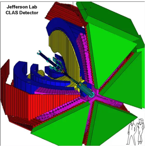
The CEBAF Large Acceptance Spectrometer (CLAS), described in detail in Ref. [11], was based on a six-coil toroidal superconducting magnet. Figure2 shows a cutaway view of the detector along the beam line. Charged particles are tracked through each of the six magnetic field regions (hereby labeled “sectors”) between its coils, with three layers of multiwire drift chambers (DC), numbered 1 to 3 consecutively from the target outward. [90].

Beyond the magnetic field region, charged particles were detected in a combination of gas Cherenkov counters, scintilla-tion counters, and total absorpscintilla-tion electromagnetic calorime-ters. There was one set of scintillation counters (SC) [91] for each of the six sectors. These were used for triggering and for time-of-flight (TOF) measurements, with a typical time resolution of 0.2–0.3 ns. In the forward region of the detector, the SC was preceded by gas-filled Cherenkov counters (CC)

FIG. 2. The CLAS spectrometer. Different colors represent dif-ferent components of the detector (from the central target outward): three layers of drift chambers (DCs) (blue) and the torus magnet (yellow), Cerenkov counters (CCs) (magenta), TOF counters (SCs) (red), and electromagnetic calorimeters (ECs) (green). The electron beam travels through the central axis from upper left to lower right.

[92] designed to distinguish electrons and pions. Finally, each sector included a total absorption sampling electromagnetic calorimeter (EC) [93] made of alternating layers of lead and plastic scintillator with a combined thickness of 15 r.l. The EC was used to measure the energy of the scattered electrons and to detect neutral particles.

Torus currents of 1500 A (at low beam energies) or 2250 A (at high beam energies) were employed in this experiment. For positive (negative) current, forward-going negative par-ticles were bent inward (outward) with respect to the beam line. The two conditions were referred to as “inbending” and “outbending,” respectively. Inbending allowed for larger acceptance of electrons at large scattering angles (high θ) and higher luminosity, whereas outbending allowed for larger acceptance at small scattering angles (lowθ). The reversibility of the magnet current also allowed systematic studies of charge-symmetric backgrounds.

E. Trigger and data acquisition

FIG. 3. Kinematic coverage inQ2_{vsxfor each of the 4 electron}

beam-energy groups in the EG1b experiment. The solid and dotted lines denote theW₌1.08 and 2.00 GeV thresholds, respectively.

(TS) generated busy gates and necessary resets, and directed all the signals to the data acquisition system (DAC). The DAC accepted event rates of 2 kHz and data rates of 25 MB/s [11]. The simple event builder (SEB), used for offline reconstruc-tion of an event, used geometric parameters and calibrareconstruc-tion constants to convert the TDC and ADC data into kinematic and particle identification data. The SEB cycled through particles in the event to search for a single trigger electron—a negatively charged particle that produced a shower in the EC. If more than one candidate was found, the one with the highest momentum was selected. This particle was traced along its geometric path back to its intersection in the target to determine the path length, which, with the assumption that its velocity v ₌c, determined the event start time. From this start time, the TOF of other particles could then be determined from the SC TDC values. The TDC values from the EC were used when SC values were not available for a given particle.

IV. DATA ANALYSIS

A. Data and calibrations

The EG1b data were collected over a 7-month period from 2000 to 2001. More than 1.5×109 _{triggers from the NH}

3 target were collected in 11 specific combinations (1.606₊, 1.606₋, 1.723₋, 2.286₊, 2.561₋, 4.238₊, 4.238₋, 5.616₊, 5.723+, 5.723−, and 5.743−) of beam energy (in GeV) and main torus polarity (+,₋), hereby referred to as “sets.” Sets with similar beam energies comprise four groups with nominal average energies of 1.6, 2.5, 4.2, and 5.7 GeV. The kinematic coverage for each of these four energy groups is shown in Fig.3.

Calibration of all detectors was completed offline according to standard CLAS procedures. These procedures use a subset of “sample” runs for each beam energy and torus polarity to determine calibration constants for all ADC and TDC channels. During analysis, these data were checked using

these constants, and additional calibrations were performed whenever necessary.

The calibration of the TOF system (needed for accurate time-based tracking) resulted in an overall timing resolution of <0.5 ns [91]. Minimization of the distance-of-closest-approach (DOCA) residuals in the DC led to typical values of 500μm for the largest cell sizes (in region 3) [90]. The EC provided a secondary timing measurement for forward-going particles, and played a role for the trigger and for particle identification [93]. The mean timing difference between the TOF and calorimeter signals was minimized, yielding an overall EC timing resolution of<0.5 ns.

After calibration, all raw data were converted into particle track information and stored (along with other essential run and event data) on data-summary tapes (DSTs).

B. Quality assessment

Quality checks were done to minimize potential bias introduced by malfunctioning detector components, changes in the target, and false asymmetries. DST data that did not meet the minimal requirements outlined in this section were eliminated from the analysis.

The electron count rate in each sector (normalized by the Faraday cup charge) was monitored throughout every run. DST files with count rates outside a prescribed range (_±5% and_±8% for beam energies <3 GeV and >3 GeV, respectively) were removed from the analysis in order to eliminate temporary problems, such as drift chamber trips, encountered during the experiment.

In order to minimize false asymmetries, the beam charge asymmetry (Q_↑−Q_↓)/(Q_↑+Q_↓) for ungated cumulative charges Q_↑(Q_↓) for positive (negative) helicities was mon-itored. A cut of±0.005 on this asymmetry ensured that the false physics asymmetry due to this effect was much smaller than 10−4_.

Electron helicities were picked pseudorandomly at 30 Hz, always in opposite helicity pairs to minimize nonphysical asymmetries. A synchronization clock bit with double the frequency identified missing bits due to detector dead time or other uncertainties, allowing ordering of the pairs (see Fig.4). All unpaired helicity states were removed from the analysis.

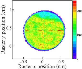
Plots of beam raster patterns were used to monitor target density and beam quality (see Fig. 5). Data obtained when raster patterns exhibited elevated count rates in regions where the beam was grazing the target cup were also excluded entirely from analysis.4

C. Event selection

As a starting point for the selection of events, particles with momentum p0.20Ebeam that fired both the CC and

4_{In one unique case where empty-target runs meeting our selection}

FIG. 4. Helicity signal logic. The clock signal (top) provided a rising edge every 30 ns. The helicity bit train (middle) was a pseudorandom stream of opposite bit pairs. The logic analyzed each helicity bit into four categories (bottom): 1, negative first bit followed by its complement; 4, positive second bit preceded by its complement; 2, positive first bit followed by its complement; and 3, negative second bit preceded by its complement. Buckets without a complementary partner were removed from the analysis.

EC triggers were treated as electron candidates. Additional criteria, discussed below, were then applied to minimize background from other particles, primarilyπ−.

1. Cherenkov counter cuts

The CCs use perfluorobutane (C4F10) gas, and have a threshold of ∼9 MeV/c for electrons and ∼2.8 GeV/c

for pions. Between these two momenta, the CC efficiently separated pions from electrons. A minimum of 2.0 detected photoelectrons (p.e.) in the CC PMTs was required for electron candidates with p <3.0 GeV/c. For particles with higher momentum, a minimum cut of 0.5 p.e. was used only to eliminate contributions from internal PMT noise.

Geometric and time matching requirements between CC signals and measured tracks were used to reduce background. These cuts on the correlation of the CC signal with the trigger-ing particle track removed the majority of the contamination

position (cm)

x

Raster

-0.5 0 0.5

position (cm)

y

Raster

0 0.5 1

0 100 200

FIG. 5. Raster pattern for a sample run, demonstrating some temporary settling of the target material. (The “crosshair” pattern is a nonphysical relic of the coordinate reconstruction.)

CC Photoelectron Signal (p.e.)

0 5 10 15 20 25 30

Counts

-3

10

0 50 100 150

200 _{before π}± _cuts

cuts

± π

after

FIG. 6. Cherenkov signal distributions before (red, solid line) and after (black, dotted line) requiring track matching.

dominating the lower part of the CC signal spectrum. The effect of these cuts is shown in Fig.6. Pion contamination at low signal heights was reduced substantially with little loss of good events.

The determination of dilution factors (see Sec. IV E 1) required a precise comparison of count rates for different targets. Therefore, detector acceptance and efficiency for runs on different targets had to remain constant. Inefficiencies in the CC were the main source of uncertainty in electron detection efficiency for CLAS. Therefore, tight fiducial cuts were developed to select the region where the CC was highly efficient. These cuts were used only for the dilution factor analysis.

The CC efficiency is defined by the integral of an assumed Poisson distribution yielding the percentage of electron tracks generating signals above the 2.0 p.e. threshold. It varied as a function of kinematics due to the CC mirror geometry. The mean value of the signal distribution was determined as a function of electron momentump and anglesθ andφusing

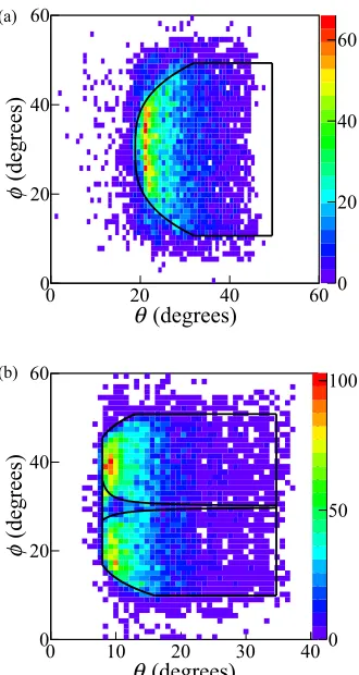
epelastic events from several CLAS runs at beam energies of 1.5–1.6 GeV. The deduced efficiency map has a plateau of high efficiency in the center of each sector, which rapidly drops off to zero at the sector edges. For the fiducial cut, we developed a function ofp,θ, andφto define a boundary enclosing events with more than 80% CC efficiency in each 0.5 GeV momentum interval (see Fig.7). Fiducial cuts were specific to each CLAS torus setting. Additional center-strip cuts in each sector were required to remove regions with inefficient detector elements.

2. Electromagnetic calorimeter cuts

Further suppression of pion backgrounds was provided by the EC, in which minimum ionizing particles (hadrons) deposited far less energy than showering electrons. A base cut was developed by observing the energyECtotdeposited in the entire EC and the energyECin deposited only in the first 5 of 13 layers (see Fig. 8). A loose cut of ECin<0.22 GeV (including the sampling fraction [93]) was used as a first step in separating pions from electrons in the calorimeter.

(degrees)

θ

0 20 40 60

(degrees)

φ

0 20 40 60

0 20 40 60

(degrees)

θ

0 10 20 30 40

(degrees)

φ

0 20 40 60

0 50 100

(b) (a)

FIG. 7. Sample fiducial cuts for (a) inbending and (b) outbending electrons, shown inφvsθfor one CLAS sector.

onECtot/pfurther reduced contributions from pions. Forp > 3 GeV, where the CC spectrum fails to differentiate pions and electrons, a strict cut ofECtot/p >0.89 was applied, while a looser cut ofECtot/p >0.74 is used atp <3 GeV. Figure9 shows these cuts for events plotted inECtot/pversus the CC photoelectron signal.

(GeV)

in

EC

0 1 2 3

(GeV)

tot

EC

0 1 2 3

0 50 100 150

FIG. 8. The total energyECtotdeposited in the EC vs the energy

ECindeposited in the inner (front) layer of the EC only for electron

candidates. The plot shows a clear separation of electrons from light hadrons (bottom left corner). A cut onECin(shown by the vertical

line) removes most of the hadron background.

CC signal (number of p.e.)

0 5 10 15 20

p

/

ECtot

E

0 0.5 1

0 200 400 600

FIG. 9. Scatter plot ofECtot/pvs CC signal, atp <3 GeV/c,

after fiducial cuts. Only events to the right and above the straight lines are kept as inclusive electrons.

3. Remainingπ−_{contamination}

The remaining pion contamination was determined as a function ofθ (5◦ bins) and p (0.3 GeV bins) as follows in eachp,θ bin: A modified, extrapolated Poisson distribution fit to our CC p.e. spectrum was subtracted from the pion “peak” seen at low p.e. values (see Fig.6) to get a low p.e. contamination estimate. Then, we analyzed only runs without the CC trigger in use, inverting all the electron selection cuts on the EC, resulting in a test sample composed nominally of pions. This sample was then normalized to the low p.e. contamination estimate at p.e.<2.0. The normalized nominal pion data provided an estimate of theπ−contamination present at p.e.>2.0, where the inclusive electrons lie. Dividing by the total number of inclusive electrons yielded the contamination fractionRp_(θ,p).

Plots of the pion contamination fractions as a function ofp

andθare shown in Fig.10. These were seldom more than 1% of the total electron count. An exponential function

R(θ,p)=ea+bθ+cp+dθp (44)

was then fit to these points. Pion contamination corrections could be made by adding

Araw=

R(θ,p)(Araw−Aπ)

1₋R(θ,p) (45)

to the raw asymmetry Araw. Since the effect is very small, and the inclusive pion asymmetryAπ is not well known, we

applied no correction and instead treatArawwithAπ =0 as

the systematic uncertainty.

4. Background subtraction of pair-symmetric electrons Dalitz decay of neutral pions [95] and Bethe-Heitler processes [96] can producee+e− pairs at or near the vertex, contaminating the inclusive e− spectrum. To determine this contamination, we assumed that the event reconstruction and detector acceptances for e+ production were identical to those for their paired e− when the main torus current was reversed, and that the overall cross section is small enough that small differences in beam energy (e.g. 2.286 vs 2.561 GeV) minimally affected the production rate.

ratio

/e

-π

3

10

50 100

o < 20

θ

< o 15

o < 25

θ

< o 20

o < 30

θ

< o 25

o < 35

θ

< o 30

o < 40

θ

< o 35

(GeV/c)

p

1

2

3

ratio

/e

-π

3

10

5 10

(a)

(b)

FIG. 10. Pion contamination fraction (a) before and (b) after track-matching cuts for the 5.7-GeV beam energies, as a function of polar angle and momentum. The increase beyondp=2.8 GeV/c

indicates the threshold beyond which pions start to produce a signal in the CC.

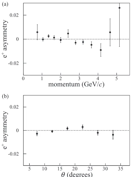
positron triggers were analyzed identically to those with electron triggers. The overall double-spin asymmetry fore+

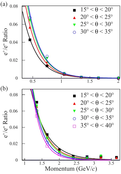
triggers was small (see Fig.11). The e+/e− contamination ratios Rp, which were largest at low momenta (Fig. 12), were fit with the parameterization of Eq. (44). Then, Eq. (45) (with Aπ →Ae+) was used to determine a multiplicative background correction factorCback≡(Araw+Araw)/Arawto convert the raw asymmetry to the background-free physics asymmetry. Here we assumed thatAe+=0, consistent with the average from our measurements (see Fig.11).

To estimate the systematic uncertainty from this back-ground, two changes were made toCbackin the reanalysis.Rp was changed by half the difference between two equivalent determinations: one using outbending electrons and inbending positrons, and the other using the opposite torus polarities for either particle. Also, Ae+ was set to a nonzero value equal to 3 times the statistical uncertainty of the averaged positron asymmetry.

5. Elastic ep→e′_{p event selection}

Both the momentum corrections (Sec. IV D 2) and the determination of beam polarization × target polarization (Sec.IV E 2) required identified elasticepscattering events. For this purpose, we selected two-particle events containing

)

c

momentum (GeV/

0 1 2 3 4 5

asymmetry

+

e

-0.02 0 0.02

(degrees)

θ

5 10 15 20 25 30 35

asymmetry

+

_e

-0.02 0 0.02

(a)

(b)

FIG. 11. Average positron asymmetries for the 5.7-GeV data set as a function of (a) momentum and (b) scattering angleθ.

an electron and one track of a positively charged particle. Electron PID cuts were relaxed to require only a minimum of 0.5 CC p.e. TheE/pEC cut thresholds were lowered to 0.56 forp <3 GeV/cand 0.74 forp >3 GeV/c. These relaxed cuts increased the statistics while the exclusivity cuts discussed below removed all pion background.

A beam-energy-dependent cut on |Mp−W| (where Mp

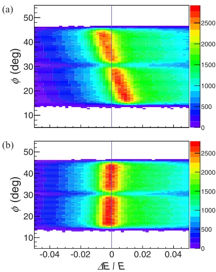
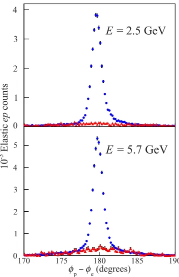
is the proton mass), which ranged from 30 MeV at 1.6 GeV to 50 MeV at 5.7 GeV, suppressed inelastic contributions. Further kinematic constraints were applied on deviations of the missing momentum p, the proton polar angle θ, and the difference between the azimuthal proton and electron angles φ, from those expected for elastic ep kinematics (see Fig.13). Final cuts ofp <0.15 GeV,θ < 1.5◦and

φ < 2.0◦identify elasticepevents, with typically less than 5% nuclear background (see Fig.22).

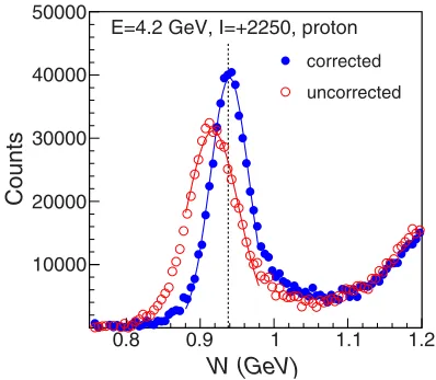
D. Event corrections

The reconstructed track parameters of each event were corrected for various distortions to extract the correct kine-matic variables at the vertex. These kinekine-matic corrections are explained in the following two subsections.

1. Phenomenological kinematics corrections

0.5 1 1.5 2

Ratio

/e

+

e

0 0.02 0.04 0.06 0.08

°

< 20

θ

<

°

15

°

< 25

θ

<

°

20

°

< 30

θ

<

°

25

°

< 35

θ

<

°

30

)

c

Momentum (GeV/

1 1.5 2 2.5 3 3.5

Ratio

/e

+

e

0 0.02 0.04 0.06

0.08

₁₅

_°

_<

_θ

_{< 20}

_°

°

< 25

θ

<

°

20

°

< 30

θ

<

°

25

°

< 35

θ

<

°

30

°

< 40

θ

<

°

35

(a)

(b)

FIG. 12. Ratios ofe+/e−as a function of electron momentump, at variousθangles, for the (a) 2.561−and (b) 5.727+data sets.

geometrical corrections to the reconstruction algorithm (for target rastering and stray magnetic fields).

Rastering varies thexyposition of the beam over the target in a spiral pattern with a radius of_∼0.5 cm (see Fig.5). The instantaneous beam position can be reliably extracted from the raster magnet current. The reconstructedz-vertex position (the

zaxis is along the beam line) and the “kick” inφwere corrected for this measured displacement of the interaction point from the nominal beam center [97], prior to the application of a nominal (₋58< vz<−52 cm) vertex cut (see Fig.14).

Collisional energy loss of both incident and scattered electrons within the target was accounted for by assuming a 2.8-MeV/(g/cm2_{) energy loss ratedE/dxfor electrons [98].} The calculation, incorporating the target mass thickness, vertex position, and polar scattering angleθ, yielded typical energy losses of∼2 MeV before and after the event vertex. The energy loss of scattered hadrons was similarly estimated using the Bethe-Bloch formula [99].

Determination of the effects of multiple scattering on kinematic reconstruction was more complex, and was studied with the GEANT CLAS simulation package GSIM [100].

For multiparticle events, an average vertex position was determined by calculating a weighted average of individual reconstructed particle vertices. Comparing each particle vertex with this average gives a best estimate for the effect of multiple scattering on that particle on its way to the first drift

) c (GeV/ elastic p

e

p

-1 -0.5 0 0.5 1

Counts

0 20 40 60

(degrees) elastic

θ

e

θ

-10 -5 0 5 10

Counts

0 20 40 60

(degrees) elastic

φ

e

φ

-10 -5 0 5 10

Counts

0 20 40 (a)

(b)

(c)

FIG. 13. Kinematic cuts on (a) the difference between measured and expected momentum, (b) polar angle, and (c) azimuthal angle of elasticepevents. Each of the distributions has the other two cuts applied.

chamber region. TheGSIMmodel was then used to generate an adjustmentdθ(θ,1/p) [101] to the measured scattering angle. TheGSIMpackage was also used to provide a leading-order correction due to magnetic field effects not incorporated into the main event reconstruction software. Particularly important is the extension of the target solenoid field into the inner layer

(cm)

z

v

-80 -70 -60 -50 -40 -30

Events

10

2

10

3

10

4

10