This is a repository copy of
The evolution of host defence to parasitism in fluctuating
environments
.
White Rose Research Online URL for this paper:
http://eprints.whiterose.ac.uk/124875/
Version: Accepted Version
Article:
Ferris, C. and Best, A. (2018) The evolution of host defence to parasitism in fluctuating
environments. Journal of Theoretical Biology, 440. pp. 58-65. ISSN 0022-5193
https://doi.org/10.1016/j.jtbi.2017.12.006
Article available under the terms of the CC-BY-NC-ND licence
(https://creativecommons.org/licenses/by-nc-nd/4.0/).
[email protected] https://eprints.whiterose.ac.uk/ Reuse
This article is distributed under the terms of the Creative Commons Attribution-NonCommercial-NoDerivs (CC BY-NC-ND) licence. This licence only allows you to download this work and share it with others as long as you credit the authors, but you can’t change the article in any way or use it commercially. More
information and the full terms of the licence here: https://creativecommons.org/licenses/
Takedown
If you consider content in White Rose Research Online to be in breach of UK law, please notify us by
Title: The Evolution of Host Defence To Parasitism in Fluctuating Environments. 1
Authors: Charlotte Ferris1, Alex Best1
2
1 School of Mathematics and Statistics, University of Sheffield, Sheffield, S3 7RH, UK
3
Corresponding Author: Charlotte Ferris, School of Mathematics and Statistics, University 4
of Sheffield, Sheffield, S3 7RH, UK. Email: [email protected] 5
Keywords: Adaptive dynamics, Host-parasite, Host evolution, Seasonality 6
Abstract: 7
Given rapidly changing environments, it is important for us to understand how the evolution of 8
host defence responds to fluctuating environments. Here we present the first theoretical study 9
of evolution of host resistance to parasitism in a classic epidemiological model where the host 10
birth rate varies seasonally. We show that this form of seasonality has clear qualitative and 11
quantitative impacts on the evolution of resistance. When the host can recover from infection, 12
it evolves a lower level of defence when the amplitude is high. However, when recovery is absent, 13
the host increases its defence for higher amplitudes. Between these different behaviours we find 14
a region of parameter space that allows evolutionary bistability. When this occurs, the level 15
of defence the host evolves depends on initial conditions, and in some cases a switch between 16
attractors can lead to different periods in the population dynamics at each of the evolutionary 17
stable strategies. Crucially, we find that evolutionary behaviour found in a constant environment 18
for this model doesn’t always hold for hosts with highly variable birth rates. Hence we argue 19
that seasonality must be taken into account if we want to make predictions about evolutionary 20
1. Introduction 22
Given the ubiquity of infectious diseases in natural systems there is strong selection pressure 23
on host organisms to evolve costly defence mechanisms. A wide range of theoretical work has 24
been developed to understand the evolution of host defence against parasitism, with much of 25
this work focused on the ecological/epidemiological feedbacks that drive selection of quantitative 26
host defence (van Baalen, 1998; Boots & Haraguchi, 1999; Boots & Bowers, 1999, 2004; Restif 27
& Koella, 2003; Miller et al., 2005, 2007; Bonds, 2006; Best et al., 2008, 2009; Carval & 28
Ferriere, 2010). These studies have explored how long-term, stable investment in host defence 29
varies with ecological/epidemiological parameters, as well as determining the conditions that 30
can lead to coexistence of strains through evolutionary branching. However, the vast majority 31
of these studies assume that the populations live in a temporally static environment. In reality, 32
almost all natural systems are subject to some degree of temporal environmental heterogeneity, 33
in particular fluctuations caused by seasonality. For example, many natural species exhibit 34
seasonal reproductive strategies driven by regular environmental fluctuations (Rowan, 1938; 35
Stawski et al., 2014; Ketterson et al., 2015; Furness, 2016). It is therefore essential that we 36
consider the impact of fluctuating environmental conditions on the evolution of host defences. 37
It is well established that variable climates affect ecological systems (Ewing et al., 2016), in-38
cluding the spread and impact of diseases (Fine & Clarkson, 1982; Finkenst¨adt & Grenfell, 39
2000; Altizer et al., 2006). Many theoretical studies have considered the effects of seasonality 40
in purely epidemiological models (i.e., non-evolutionary), often through a periodic transmission 41
rate (Schwartz & Smith, 1983; Aron & Schwartz, 1984; Olsen & Schaffer, 1990). Increasing the 42
amplitude of the transmission rate can generate sub-harmonic oscillations or cause the popula-43
tion dynamics to move through a series of period-doubling bifurcations, eventually leading to 44
chaotic dynamics (Grossman, 1980; Schwartz & Smith, 1983; Greenman et al., 2004; Grassly 45
& Fraser, 2006; Childs & Boots, 2010). Small perturbations in these seasonal models can also 46
trigger the system to switch between distinct attractors, often due to resonance, potentially 47
leading to significant changes in the population dynamics and different patterns of outbreaks 48
(Smith, 1983; Schwartz, 1985; Keeling et al., 2001; Kamo & Sasaki, 2002; Greenman et al., 49
2004). These complex dynamics have been found to exist less frequently when seasonality is 50
assumed to occur in the host birth rate rather than transmission (White et al., 1996; Begon et 51
the impact of a disease are likely to be more accurate when either of these types of seasonality 53
are included in the model (White et al., 1996; Kamo & Sasaki, 2002). 54
There is an increasing appreciation of the importance of temporal heterogeneity in host-enemy 55
interactions within the experimental evolution literature (Blanford et al., 2003; Friman & Laakso, 56
2011; Hiltunen et al., 2012; Harrison et al., 2013), for example showing that rapidly fluctuat-57
ing environments constrain co-evolutionary arms races in a bacteria-phage system (Harrison et 58
al., 2013). Theoretically, however, evolution and seasonality have rarely been studied together 59
in a host-parasite context. The few studies that do exist have either investigated evolution 60
of only the parasite (Koelle et al., 2005; Sorrell et al., 2009; Donnelly et al., 2013), or used 61
a genetic-based, rather than ecology-driven, model for evolution of the host (Nuismer et al., 62
2003; Mostowy & Engelst¨adter, 2011; but see Poisot et al., 2012). Seasonality in the host’s 63
birth rate does not affect the evolution of the parasite’s transmission/virulence strategy un-64
less a density-dependence is applied to virulence (parasite-induced mortality) (Donnelly et al., 65
2013). This occurs because the average susceptible density, and therefore the parasite fitness, 66
doesn’t depend on the seasonal parameters unless this density-dependence is included. Else-67
where, step-wise environmental variation implemented through a dynamic resource was found 68
to change the coevolutionary outcomes in a gene-for-gene based host-parasite system (Poisot et 69
al., 2012). In particular, they found that both the host and parasite invest more in resistance 70
and infectivity respectively for higher amplitudes in the seasonality. However, we currently have 71
no theory specifically addressing the impact that seasonality has on the evolution of host defence 72
to parasitism. 73
Here we investigate the impact of a continuous seasonal birth rate on the evolution of quantitative 74
host avoidance through small mutation steps using an evolutionary invasion (adaptive dynamics) 75
method. We use a classic SIS (Susceptible-Infected-Susceptible) model, and focus on how the 76
amplitude and period of the implemented seasonality impacts the ecological/epidemiological 77
dynamics, and therefore the evolution of the host. 78
2. Methods 79
The population is modelled using an SIS (susceptible-infected-susceptible) framework with the 80
dS
dt =a(1−qN)S−bS−βSI+γI, (1)
82
dI
dt =βSI−(b+α+γ)I, (2)
whereS and I are the susceptible and infected population sizes respectively, and N =S+I is 83
the total population size (Anderson & May, 1981). All offspring are born susceptible at ratea, 84
and only susceptible hosts are able to reproduce, i.e. the parasite renders the host (temporarily) 85
sterile. The births are limited by density with crowding coefficient q, so that birth rate is low 86
when competition is high. All hosts die at baseline mortality rateb, with an additional infected 87
death rate α. The parasite is transmitted to susceptible hosts at rate βI due to contact with 88
infected individuals. Hosts recover from the parasite at rate γ and return to the susceptible 89
class with no acquired immunity. Default parameter values are given in table 1. 90
We assume that seasonality occurs on the ecological timescale, so to incorporate this we let the 91
birth rate depend periodically on timet: 92
a=a(t) =a0(1 +δsin(2πt/ǫ)), (3)
where a0 is the average birth rate, δ ∈ [0,1] is the amplitude and ǫ > 0 is the period of the
93
forcing. Periodic birth rates have been observed in a large number of species (Rowan, 1938; 94
Ketterson et al., 2015), and this type of function has been used many times to model a time-95
varying birth rate (He & Earn, 2007; Donnelly et al., 2013; Dor´elien et al., 2013) or transmission 96
rate (Schwartz & Smith, 1983; Grassly & Fraser, 2006; Childs & Boots, 2010). For our default 97
Parameter Definition Default Value
ˆ
a0 Trade-off coefficient in the average birth rate 108
p Trade-off coefficient in the average birth rate 103.75
c Trade-off coefficient in the average birth rate 1.5
β Transmission coefficient Varies
βmin Minimum transmission coefficient 0.5
βmax Maximum transmission coefficient 10
δ Amplitude of the birth rate forcing Varies
ǫ Period of the birth rate forcing 1
q Crowding coefficient acting on births 0.1
b Baseline mortality rate 1
γ Recovery Rate Varies
α Virulence/additional death rate due to parasite 1
parameter values, the periodǫis the same as the average lifespanb(1 year), but see section 3.4 98
for varyingǫor Appendix F for alternativeb. 99
We assume that the host evolves defence through the transmission coefficient (avoidance)β. We 100
let the average birth rate depend on this as a trade-off so that there is a cost to resisting the 101
parasite, as there is experimental support for such a relation to exist (Boots & Begon, 1993). 102
We use the following trade-off function based on that used by White et al. (2006): 103
a0=a0(β) = ˆa0−p
(1 + β−βmin
βmax−βmin) (1 +c β−βmin
βmax−βmin)
, (4)
where ˆa0 > 0, 0 < p < aˆ0, c > 1 and β ∈ [βmin, βmax]. a0(β) has minimum ˆa0 −p, and
104
parameters p, c determine the gradient and curvature of the trade-off, which needs to have 105
positive gradient: as the host invests in defence against the parasite (β decreases), less can be 106
invested in reproduction (a0(β) decreases) (Boots & Haraguchi, 1999; Geritz et al., 2007). The
107
constraints on the trade-off parameters give accelerating costs of defence, so that it is more costly 108
to invest in resistance when defence is already highd 2
a0(β)
dβ2 <0
, see figure A.1 in Appendix 109
A. Accelerating trade-offs generally lead to evolutionary attractors (Hoyle et al., 2008), which 110
will be our focus here. 111
We use the adaptive dynamics method to study evolution of the host in the transmission coef-112
ficient β. The method involves adding a rare mutant with susceptible and infected population 113
sizesSm,Imand transmission coefficientβmvery close to the resident transmission coefficientβ.
114
We assume that mutants occur infrequently so that the resident population reaches the dynamic 115
attractor of the population dynamics (generally a limit cycle here) before the next mutant is 116
introduced (Geritz et al., 1998). When a new mutant arises, it is rare compared to the current 117
population, so we assume that the resident remains at its limit cycle as long as the mutant 118
population is small (Geritz et al., 1998). To analyse how the host evolves, we consider the mu-119
tant’s fitness, defined to be the long-term exponential growth rate of the mutant in the current 120
environment (Metz et al., 1992). 121
In the case where γ = 0, the fitness is relatively simple to find. We no longer have infected 122
mutants (they are absorbed intoI), and we can read off the time-varying growth rater(t) of the 123
mutant host from the linearisation of the equation for the susceptible mutant (dSm/dt=r(t)Sm,
124
of this over one period to find the mutant fitness: 126
r= 1
T
Z P1
P0
r(t)dt= a0(βm)
T
Z P1
P0
1 +δsin
2πt ǫ
[1−qN(t)]
dt−b−βm T
Z P1
P0
I(t)dt , (5)
where T is the period of the system, P0 is an arbitrary time after the resident dynamics have
127
reached a limit cycle, andP1 =P0+T.
128
Unfortunately we cannot use this averaging method whenγ >0. Instead, we have to find the 129
Lyapunov exponents or Floquet multipliers numerically (Metz et al., 1992; Klausmeier, 2008). 130
We do this by letting the linearly independent solutions of the linearised mutant equations be 131
of the form Xi(t) =eµitpi(t) fori∈1,2 (Grimshaw, 1990), and then take the largestµi as the
132
mutant fitness. A full discussion of the method is given in Appendix B. We also ran stochastic 133
simulations which relax the separation of timescales assumption, and these confirm our key 134
results, for examples see figure 2 and Appendix D. 135
3. Results 136
3.1. Population dynamics
137
To explore how the population dynamics shape selection, we first consider the nature of the 138
attractors of equations (1) - (2). For most parameter sets, the period of the population dynamics 139
is equal to that of the forcing in the birth rate, i.e.T =ǫ. However, there are parameter regions 140
where the population undergoes a period-doubling bifurcation with resulting cycles of period 141
T = λǫ for some positive integer λ. We can also find cases of multiple attractors, often with 142
different periods. After finding this period, we can write down the average size of each class as 143
follows (method in Appendix C): 144
ˆ
S = 1
T
Z P1
P0
S(t)dt= α+b+γ
β (6)
145
ˆ
I = 1
T
Z P1
P0
I(t)dt= β (α+b+γ)T
Z P1
P0
SIdt . (7)
Immediately we can see that the average susceptible population ˆS does not depend on either of 146
which we have to evaluate numerically for δ > 0. For the default parameter values in table 1, 148
we find that ˆI increases with the amplitude of seasonality δ, and hence the average prevalence 149
1
T
RP1
P0
I(t)
N(t)dt
of the parasite also increases. When we vary the period ǫ, ˆI increases to a peak 150
atǫ≈1.5 due to resonance with the unforced system, then decreases asǫcontinues to increase.
151
This is discussed further in section 3.4. Considering the fitness expression in (5), it is clear that 152
the effect of seasonality on these population averages will have crucial impacts on host evolution 153
for all recovery values, unlike with parasite evolution (Donnelly et al., 2013). We can therefore 154
use these averages to explain how the host evolves in response to changes in parameters. 155
3.2. Evolution for γ = 0 156
When we setγ = 0, we revert back to the simpler SI model. As stated in section 2, we can write 157
down the fitness of the host in this case for all δ∈[0,1] in equation (5). Here we only consider
158
continuously stable strategies (CSSs) unless stated otherwise, i.e. singular points that are both 159
evolutionarily stable (ES) and convergence stable (CS) as defined by Geritz et al. (1998) which 160
lead to long-term evolutionary attractors. This behaviour was confirmed using pairwise-invasion 161
plots (PIPs) and simulations over a range of parameters, for an example see Appendix D. 162
Whenδ is increased from 0, we find that the average infected population increases and so does 163
the investment in defence (i.e.β∗ decreases & higher defence), see figure 1(a),(b). This is what
164
we would naively expect: as the average infected population increases, the host has to invest 165
more in resistance against the parasite to reduce the proportion of infected individuals (Boots 166
& Haraguchi, 1999; Boots et al., 2009). 167
In section 3.1 we mentioned that for particular parameter sets, period-doubling bifurcations and 168
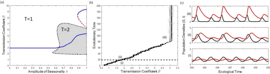
bistability between different attractors in the population dynamics can occur. Figure 1(c),(d) 169
shows an example of this phenomenon together with host selection. As we increase δ, there 170
is a point at which the 1-year solution undergoes a period-doubling bifurcation. The resulting 171
2-year solution then goes through two folds, after which a stable solution exists, see Appendix E. 172
Bistability between different solutions for δ ∈(0.57,0.63) causes overlap of the singular points
173
given by each cycle, giving a discrete change in the CSS resistance β∗ and average infected
174
population, figure 1(c),(d). Note that due to the basins of attraction for each CSS within 175
the bistability region, the host can only evolve towards the T = 2 singular point for initial 176
transmission coefficientβ0 greater than the lower bound of the bistablility region, see Appendix
Figure 1: Change in (a),(c) the singular pointβ∗ and (b),(d) the average infected population forβ=β∗as the
amplitude of seasonalityδvaries forγ= 0. Default parameters were used in (a),(b), with ˆa0= 104 in (c),(d). In
(c),(d), on the left only the 1-year solution is stable, and on the right only the 2-year solution. In the centre there is bistability between the 1 and 2-year cycles or between the two different 2-year cycles. Blue - periodT= 1; Red - periodT = 2.
E. This jump in the average infected population and singular point occurs whenever a period-178
doubling bifurcation and bistability between attractors exists forγ = 0. 179
Overall the impact of the amplitude of seasonalityδ on the singular point forγ = 0 is weak for 180
a wide range of parameters as seen in figure 1. Seasonality has a much stronger effect for higher 181
recovery rates, as discussed below. 182
3.3. Evolution for γ >0 183
Unlike in the SI model above, when γ > 0 we use a numerical approximation to find the 184
host fitness. When γ is relatively close to zero, we find one singular point which decreases as 185
δ increases, as seen in section 3.2. However for positive but small values of γ, this behaviour 186
changes direction. We start to see both the singular pointβ∗ and the average infected population
187
increasing, in contrast toγ = 0 where the trends go in opposite directions. As recovery increases, 188
selection for defence is weakened, and so at this small recovery maintaining a large population 189
in evolutionary direction. 191
Figure 2: (a) Change in the singular points asδ varies for ˆa0 = 104, γ = 0.005. Blue lines indicate the CSS
points, red dashed lines the repeller point and black dotted lines the switch between attractors. The period of the population dynamics is 2 in the shaded region and 1 (ǫ) elsewhere. (b) Simulation example corresponding to (a) with initial transmission coefficientβ0 = 0.7 andδ= 0.9, which evolves towards the lowest CSSβ∗L= 5.067.
Darker squares indicate a higher proportion of the population with the corresponding transmission coefficientβ, and the dashed line marks the point where evolution drives the population to switch to an attractor with period T = 2. (i)-(iii) correspond to sample population dynamics of the resident strain shown in (c), with black for S and red forIat evolutionary times (i) 10, (ii) 20 and (iii) 100.
As we continue to increase the recovery rate, we reach a region ofγ values where three singular 192
points exist, two CSSs with a repeller between them, for an example see figure 2(a). Here we 193
have evolutionary bistability between two CSSs, and for certain parameter sets the CSSs have 194
different cycle lengths due to the stability of the attractors in the population dynamics, as in 195
the example shown. In this case the host could start in a 1-year cycle, but evolution would 196
drive it into a 2-year regime, i.e. evolution can drive changes in the population dynamics, see 197
figure 2(b),(c). We can also have the situation where all three singular points give period two 198
population dynamics (not shown). Figure 3 shows two-dimensional contour plots for two CSS 199
points in the parameter regions where they occur. Both CSS points increase withδ, as argued 200
above, but they go in opposite directions as γ increases. This occurs because at high levels of 201
defence (low β∗, figure 3(a)), selection for even higher defence weakens as recovery increases,
202
and so the host decreases its resistance. However, when the host has a low level of defence (high 203
β∗, figure 3(b)), the susceptible hosts become infected more quickly and an increase in recovery
204
raises the infected population further, hence there is strong selection for defence and the host 205
invests more in resistance. Recovery therefore has a much more complicated effect on evolution 206
when seasonality is included in the model, since most of these bistability regions occur for large 207
amplitudes. 208
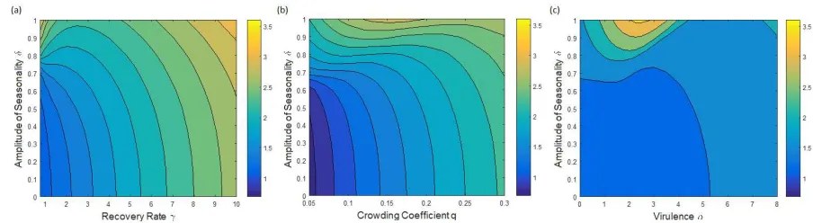
If we increaseγ further, the size of the interval ofδ values where bistability occurs decreases to 209
zero. For allγ values above this point, we find only one singular point β∗ that increases with δ,
[image:10.612.70.513.98.219.2]Figure 3: Two-dimensional contour plots showing the change in the two CSS points that occur asγandδvary for default parameters. (a)β∗
L, the smallest CSS point; (b)β∗H, the highest CSS point. White areas indicate where
each singular point does not exist.
figure 4(a), for the same reasons as explained above. 211
Figure 4(a) shows a two-dimensional contour plot for the singular point β∗ as δ and γ vary
212
in the region where one singular point exists. For the majority of amplitudes, the average 213
infected population decreases with increasing recovery, and hence the host invests less in defence. 214
However, we have slightly more complicated behaviour for highδ. Initially we find that the host 215
increases defence (decreasesβ∗), then at an intermediate recovery the trend turns and the host
216
decreases its defence (increases β∗). This behaviour is due to changes in the average infected
217
population, which peaks for intermediateγ since initially the increase in susceptible individuals 218
available to be infected outweighs the loss from recovery. 219
Figure 4: Two-dimensional contour plots showing the value of the singular pointβ∗ as amplitude of seasonality
δand (a) recovery rateγ, (b) crowding factorqand (c) virulenceαvary. Other parameters were fixed at default values from table 1 withγ= 1.
Alterations to other model parameters also causes variation in the host’s evolution. Figure 4(b) 220
shows the change in the singular point β∗ as δ and the crowding coefficient q are varied. As
221
above, we see thatβ∗ increases withδfor all values ofq. As we increaseqfor fixedδ, the infected
222
[image:11.612.46.526.287.625.2] [image:11.612.65.517.488.612.2]i.e. β∗ to increase, which is exactly what we find for most values of δ. However, for very high
224
amplitudes we find that the level of defence has a more complicated relationship with q, and 225
in particular that defence is minimal (β∗ maximum) for intermediate and very high values of
226
q. For low q, the average infected population decreases as q increases, hence the host invests 227
less in defence as for lowerδ. However, there comes a point where the susceptible population is 228
relatively low due to the decreased resistance, and so the host invests more in defence rather than 229
births to increase the average susceptible population. As q continues to increase, the average 230
infected population becomes small enough that selection for defence is weakened, and so the 231
host returns to its previous behaviour and invests less in defence (β∗ increases) for very high q.
232
We find similar results when the virulence α varies, figure 4(c). As α increases, the average 233
infected population decreases and the host can afford to invest less in defence, which is exactly 234
what we find for δ up to intermediate values. However, as for varying q, the trend becomes 235
more complicated for highly seasonal birth rates. In this region, we now have a large peak inβ∗
236
for an intermediate value ofα, followed by a trough and a small increase inβ∗ for high α. For
237
small and very largeα, this behaviour is due to the average infected population decreasing and 238
therefore the host can afford to invest less in defence. However, the initial behaviour causes the 239
total population to decrease, and there is a region of α values where the host needs to evolve 240
in such a way that the population size increases. Therefore the host has to balance changes in 241
the infected and total population sizes, giving the more complicated evolutionary behaviour for 242
high amplitudes. 243
The results discussed above are for a parameter set where the host lifespan is equal to the period 244
of forcing (one year). The effects seen are dampened for longer lived hosts (smallerb), and there 245
can be no difference in the evolutionary behaviour with γ, q orα for different amplitudes (see 246
Appendix F). Hence the effect of the amplitude on the host’s evolutionary behaviour with other 247
parameters depends on context, and in particular we cannot rely on the behaviour remaining 248
the same as the amplitude of the birth rate increases for short-lived hosts. 249
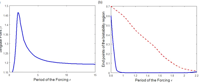
3.4. Varying the Period of the Forcingǫ
250
The population dynamics have period determined by that of the forcing ǫ, as discussed in 251
section 3.1. We can investigate how changing this period over a wide range of values affects the 252
Figure 5: (a) Change in the CSS singular pointβ∗as ǫvaries for default parameters withδ= 0.5 &γ = 1. (b)
Change in the size of the bistability region in recovery rateγ asǫvaries. Blue: γvalue where bistability starts; Red dashed: γvalue where bistability ends.
most appropriate). We found that there is a large peak in both the average infected population 254
and the singular point β∗ caused by resonance with the natural timescale of the model, after
255
which they decrease slowly as ǫ is increased further. Hence for rapidly changing environments 256
(ǫlow), any alteration to the period would have a significant impact on the host’s evolution. In 257
comparison, for slowly varying environments any change in the period barely alters the host’s 258
evolution. This behaviour with ǫ stays roughly the same for all parameters tested. Similarly, 259
when both the period and other parameters are varied simultaneously, the period doesn’t affect 260
the evolutionary behaviour we find as other parameters change and vice versa. 261
The bistability region studied in section 3.3 changes in size for varying period ǫ. Figure 5(b) 262
shows this, indicating that the bistability region is largest (in γ) for ǫ≈1, slightly lower than
263
the peak seen in figure 5(a). Above and below this value the bistability region decreases in size 264
and quickly disappears. The period of the seasonality therefore has a large impact on whether 265
or not these bistability regions occur. 266
4. Discussion 267
We have shown that seasonality in the ecological dynamics, specifically the birth rate, has a 268
clear quantitative and qualitative effect on the evolution of host resistance against a parasite 269
in our model. The relative size and nature of the impact depends crucially on the underlying 270
epidemiological model, and particularly on the potential for recovery from infection. We found 271
regions of parameter space where there is bistability between two distinct evolutionary strategies 272
[image:13.612.123.473.74.221.2]In these regions, evolution could drive the population to a different attractor, fundamentally 274
altering the population dynamics the host experiences. Crucially, we also found that well known 275
patterns for the host’s evolutionary strategy in a constant environment don’t necessarily hold 276
for variable birth rates, particularly when the amplitude of fluctuations is high. 277
We found that the amplitude of the seasonality and the recovery rate are key processes affecting 278
the evolution of the host’s defence for a seasonal birth rate in our model. When recovery is 279
absent, the host invests more in defence as the amplitude of seasonality increases as this leads 280
to an increase in the average infected population and thus selection for increased defence. The 281
trends observed were weak, but are consistent with existing theory on the evolution of avoidance 282
in the absence of recovery (Boots & Haraguchi, 1999; Donnelly et al., 2015). When the host 283
can recover from the parasite, the evolutionary dynamics become more complicated. The trend 284
of host investment with the amplitude of seasonality switches direction at a low recovery rate, 285
above which the host decreases its defence as the amplitude increases, since the host is now 286
balancing reduced transmission against the increased contribution to fitness made by infected 287
hosts through recovery. These results emphasise the importance of recovery in host-parasite 288
infections as they prevent the parasite from being a ’functional predator’ (Boots, 2004; Donnelly 289
et al., 2015; Best et al., 2017). We also note that our results with recovery for host evolution are 290
similar to the findings of Donnelly et al. (2013) for parasite evolution, where the parasite invests 291
more in infectivity as the amplitude of seasonality increases. This suggests a robust result that 292
in many systems increased seasonal amplitude will lead to higher transmission, though a full 293
coevolutionary study that includes recovery would be needed to confirm this. 294
There has been a lack of attention to how seasonality might affect host evolution in theoretical 295
studies, even though it has been shown that epidemiological dynamics can be greatly impacted 296
by a variable environment (Altizer et al., 2006; Grassly & Fraser, 2006). In addition, it is well 297
known that a wide range of species reproduce seasonally due to environmental fluctuations, for 298
example in bats (Stawski et al., 2014), killifish (Furness, 2016) and birds (Ketterson et al., 2015). 299
The theorectical studies that do consider seasonality are generally co-evolutionary with a gene-300
for-gene based infection interaction (Nuismer et al., 2003; Mostowy & Engelst¨adter, 2011; Poisot 301
et al., 2012). Of particular relevance to our study, Poisot et al. (2012) include explicit ecological 302
dynamics in their model, using an additional resource variable with discrete fluctuations to 303
different underlying assumptions, they too find that the host invests more in defence when the 305
amplitude of the seasonality is high and there is no recovery. Moreover, in an experimental study, 306
Blanford et al. (2003) showed that pea aphids,Acyrthosiphon pisum, evolved higher resistance 307
against a fungal pathogen,Erynia neoaphidis, when periodically exposed to higher temperatures. 308
Since the fecundity of aphids varies with temperature (Ramalho et al., 2015) and aphids lack 309
many of the genes associated with immune response to microbes (Gerardo et al., 2010), these 310
results agree with the theoretical results found here and by Poisot et al. (2012), that increased 311
seasonality leads to increased resistance in the absence of recovery. 312
Interestingly, we found that evolutionary bistability can exist between two convergence stable 313
strategies for small recovery rates. When the amplitude of the birth rate is high, the host may 314
evolve towards either of two levels of defence depending on initial conditions. This bistability 315
only occurs for a finite range of amplitudes, meaning that a small change in the amplitude could 316
lead to a large change in the level of defence the host evolves. Furthermore, the bistability 317
can occur in conjunction with a switch between attractors with different cycle lengths, with the 318
higher level of defence (lower transmission) giving a regime of two-year cycles in the population 319
dynamics, whereas the lower defence (higher transmission) is in a one-year regime, meaning that 320
evolution can in fact drive the population dynamics into a cycle with a different period. This 321
effect of evolution moving host-parasite systems into regions of qualitatively different population 322
dynamics has also been shown in systems which assume a constant environment but population 323
cycles occur naturally (Hoyle et al., 2011; Best et al., 2013). These results emphasize that 324
ecology/epidemiology and evolution are involved in a two-way feedback, as not only does ecology 325
drive selection, but evolution can determine the nature of the population dynamics. 326
There have been many studies considering the evolution of host defence against parasites that 327
did not include seasonality (van Baalen, 1998; Boots & Bowers, 1999; Boots & Haraguchi, 1999). 328
We have shown here that many classic results are likely to be true in a weakly seasonal system, 329
but may not hold for an increasingly variable birth rate. For example, as virulence varies, 330
investment in resistance decreases as found previously (Boots & Haraguchi, 1999; Best et al. 331
2017) for low amplitudes of seasonality, but at high amplitudes is maximized at either minimum 332
or relatively high virulence. We see similar behaviour for varying crowding factor, in that our 333
results agree with those found by Boots & Haraguchi (1999) for low amplitudes, but disagree for 334
population sizes and selection which alter the costs/benefits of resistance and births. However, 336
we have shown that this effect is dampened for hosts with longer lifespans, returning to the 337
behaviours seen in previous work for all amplitudes of the seasonality (see Appendix F). It is 338
clear that while many results found for constant environments remain true when the birth rate 339
is variable in time, this may not be the case when the amplitude is particularly high, especially 340
for short-lived hosts. 341
We also investigated the impact of changing the period of the forcing on the evolution of the 342
host’s defence. We found that changing the period induces a peak in the infected density, caused 343
by resonance in the population dynamics with the unforced system. Naively we would expect 344
this to lead to a maximum level of investment in defence, however, as with varying amplitude 345
in the presence of recovery, the host evolves towards a minimum level of defence in order to 346
maintain a large overall population size through increased birth rate. Near the peak, small 347
alterations in the period will lead to relatively large changes in the evolutionary investment in 348
defence. Away from the peak, the curve is almost flat and so the host’s evolution is barely 349
affected by changes in the period when it is already large. In an experimental study, Harrison 350
et al. (2013) found that resistance of P. fluorescens SBW25 to a phage was constrained most 351
strongly in rapidly fluctuating environments, while Duncan et al. (2017) showed that resistance 352
of the same bacteria evolved more quickly in rapidly fluctuating environments. It is unclear to 353
what extent our results agree with these experimental studies, in part due to these systems being 354
co-evolutionary with genetic specificity, and in part because it is difficult to ascertain which side 355
of the resonance peak these studies may be focusing on. It is clear, though, that the time-frame 356
of the fluctuations has important consequence to the evolutionary outcome. 357
Temporal heterogeneity, including seasonal fluctuations, are a fundamental aspect of all natural 358
ecological systems. However, both experimental and theoretical studies have rarely investigated 359
the impact of fluctuating environments on evolutionary patterns. Here we have shown that a 360
seasonal birth rate has a significant qualitative impact on the evolution of host defence in an 361
SIS model, which is highly dependent on the presence and size of recovery. It is clear that 362
key features of evolutionary dynamics may be missed by assuming a constant environment, and 363
therefore important for us to consider how seasonality may impact host-parasite evolution more 364
widely. There is clearly scope for further theoretical and experimental work to explore the 365
AcknowledgementsWe thank Mike Brockhurst and Dylan Childs for comments on an earlier 367
version of the manuscript. This work was funded by The Leverhulme Trust. 368
[1] S. Altizer, A. Dobson, P. Hosseini, P. Hudson, M. Pascual, and P. Rohani. Seasonality and 369
the dynamics of infectious diseases. J. Anim. Ecol., 9:467–484, 2006. doi: 10.1111/j.1461-370
0248.2005.00879.x. 371
[2] R.M. Anderson and R.M. May. The population dynamics of microparasites and their in-372
vertebrate hosts. Phil. Trans. R. Soc. B., 291:451–524, 1981. doi: 10.1098/rstb.1981.0005. 373
[3] J.L. Aron and I.B. Schwartz. Seasonality and period-doubling bifurcations in an epidemic 374
model. J. Theor. Biol., 110:665–679, 1984. doi: 10.1016/S0022-5193(84)80150-2. 375
[4] M. Begon, S. Telfer, M.J. Smith, S. Burthe, S. Paterson, and X. Lambin. Seasonal host 376
dynamics drive the timing of recurrent epidemics in a wildlife population. Proc. R. Soc.
377
B., 276:1603–1610, 2009. doi: 10.1098/rspb.2008.1732. 378
[5] A. Best, H. Tidbury, A. White, and M. Boots. The evolutionary dynamics of within-379
generation immune priming in invertebrate hosts. J. R. Soc. Interface, 10:20120887, 2013. 380
doi: 10.1098/rsif.2012.0887. 381
[6] A. Best, A. White, and M. Boots. Maintenance of host variation in tolerance 382
to pathogens and parasites. Proc. Natl. Acad. Sci., 105:20786–20791, 2008. doi: 383
10.1073/pnas.0809558105. 384
[7] A. Best, A. White, and M. Boots. The implications of coevolutionary dynamics to host-385
parasite interactions. Am. Nat., 173:779–791, 2009. doi: 10.1086/598494. 386
[8] A. Best, A. White, and M. Boots. The evolution of host defence when parasites impact 387
reproduction. EER, 18:393–409, 2017. 388
[9] S. Blanford, M.B. Thomas, C. Pugh, and J.K. Pell. Temperature checks the red queen? 389
Resistance and virulence in a fluctuating environment. Ecology Letters, 6:2–5, 2003. doi: 390
10.1046/j.1461-0248.2003.00387.x. 391
[10] M. Boots and M. Begon. Trade-offs with resistance to a granulosis virus in the indian meal 392
moth, examined by a laboratory evolution experiment.Functional Ecology, 7:528–534, 1993. 393
[11] M. Boots, A. Best, M.R. Miller, and A. White. The role of ecological feedbacks in the 395
evolution of host defence: what does the theory tell us? Phil. Trans. R. Soc. B., 364:27–36, 396
2009. doi: 10.1098/rstb.2008.0160. 397
[12] M. Boots and R.G. Bowers. Three mechanisms of host resistance to microparasites - avoid-398
ance, recovery and tolerance - show different evolutionary dynamics.J. Theor. Biol., 201:13– 399
23, 1999. doi: 10.1006/jtbi.1999.1009. 400
[13] M. Boots and R.G. Bowers. The evolution of resistance through costly acquired immunity. 401
Proc. R. Soc. Lond. B., 271:715–723, 2004. doi: 10.1098/rspb.2003.2655. 402
[14] M. Boots and Y. Haraguchi. The evolution of costly resistance in host-parasite systems. 403
Am. Nat., 153:359–370, 1999. doi:10.1086/303181. 404
[15] D. Carval and R. Ferriere. A unified model for the coevolution of resistance, tolerance and 405
virulence. Evolution, 64:2988–3009, 2010. doi: 10.1111/j.1558-5646.2010.01035.x. 406
[16] D.Z. Childs and M. Boots. The interaction of seasonal forcing and immunity and 407
the resonance dynamics of malaria. J. R. Soc. Interface, 7:309–319, 2010. doi: 408
10.1098/rsif.2009.0178. 409
[17] R. Donnelly, A. Best, A. White, and M. Boots. Seasonality selects for more acutely virulent 410
parasites when virulence is density dependent. Proc. R. Soc. B., 280:20122464, 2013. doi: 411
10.1098/rspb.2012.2464. 412
[18] R. Donnelly, A. White, and M. Boots. The epidemiological feedbacks critical to the evolution 413
of host immunity. J. Evol. Biol., 28:2042–2053, 2015. doi: 10.1111/jeb.12719. 414
[19] A.M. Dor´elien, S. Ballesteros, and B.T. Grenfell. Impact of birth seasonality on dynamics 415
of acute immunizing infections in sub-saharan africa. PLoS ONE, 8:e75806, 2013. doi: 416
10.1371/journal.pone.0075806. 417
[20] S.M. Duke-Sylvester, L. Bolzoni, and L.A. Real. Strong seasonality produces spatial asyn-418
chrony in the outbreak of infectious diseases. J. R. Soc. Interface, 8:817–825, 2011. doi: 419
10.1098/rsif.2010.0475. 420
become cold spots: coevolution in variable temperature environments.J. Evol. Biol., 30:55– 422
65, 2017. doi: 10.1111/jeb.12985. 423
[22] D.A. Ewing, C.A. Cobbold, B.V. Purse, M.A. Nunn, and S.M. White. Modelling the effect 424
of temperature on the seasonal population dynamics of temperate mosquitoes. J. Theor.
425
Biol., 400:65–79, 2016. doi: 10.1016/j.jtbi.2016.04.008. 426
[23] P.E.M. Fine and J.A. Clarkson. Measles in england and walesi: an analysis of factors 427
underlying seasonal patterns. Int. J. Epidemiol., 11:5–14, 1982. doi: 10.1093/ije/11.1.15. 428
[24] B.F. Finkenst¨adt and B.T. Grenfell. Time series modelling of childhood diseases: a dynam-429
ical systems approach. Appl. Stat., 49:182–205, 2000. doi: 10.1111/1467-9876.00187. 430
[25] V-P. Friman and J. Laakso. Pulsed-resource dynamics constrain the evolution of predator-431
prey interactions. Am. Nat., 177:334–345, 2011. doi: 10.1086/658364. 432
[26] A.I. Furness. The evolution of an annual life cycle in killifish: adaptation to ephemeral 433
aquatic environments through embryonic diapause. Biol. Rev., 91:796–812, 2016. doi: 434
10.1111/brv.12194. 435
[27] N.M. Gerardo et al. Immunity and other defenses in pea aphids, acyrthosiphon pisum. 436
Genome Biology, 11:R21, 2010. doi: 10.1186/gb-2010-11-2-r21. 437
[28] S.A.H. Geritz, E. Kisdi, G. Mesz´ena, and J.A.J. Metz. Evolutionarily singular strategies 438
and the adaptive growth and branching of the evolutionary tree. Evol. Ecol., 12:35–57, 439
1998. doi: 10.1023/A:1006554906681. 440
[29] S.A.H. Geritz, E. Kisdi, and P. Yan. Evolutionary branching and long-term coexistence 441
of cycling predators: critical function analysis. Theor. Pop. Biol., 71:424–435, 2007. doi: 442
10.1016/j.tpb.2007.03.006. 443
[30] N.C. Grassly and C. Fraser. Seasonal infectious disease epidemiology. Proc. R. Soc. B., 444
273:2541–2550, 2006. doi: 10.1098/rspb.2006.3604. 445
[31] J. Greenman, M. Kamo, and M. Boots. External forcing of ecological and epi-446
demiological systems: a resonance approach. Physica D., 190:136–151, 2004. doi: 447
[32] R. Grimshaw.Nonlinear Ordinary Differential Equations.Blackwell Scientific Publications, 449
1990. ISBN 0-632-02708-8. 450
[33] Z. Grossman. Oscillatory phenomena in a model of infectious diseases. Theor. Population
451
Biol., 18:204–243, 1980. 452
[34] E. Harrison, A-L. Laine, M. Hietala, and M.A. Brockhurst. Rapidly fluctuating environ-453
ments constrain coevolutionary arms races by impeding selective sweeps. Proc. R. Soc. B., 454
280:20130937, 2013. doi: 10.1098/rspb.2013.0937. 455
[35] D. He and D.J.D. Earn. Epidemiological effects of seasonal oscillations in birth rates.Theor.
456
Pop. Biol., 72:274–291, 2007. doi: 10.1016/j.tpb.2007.04.004. 457
[36] T. Hiltunen, V-P. Friman, V. Kaitala, J. Mappes, and J. Laakso. Predation and resource 458
fluctuations drive eco-evolutionary dynamics of a bacterial community. Acta Oecol., 38:77– 459
83, 2012. doi: 10.1016/J.Actao.2011.09.010. 460
[37] A. Hoyle, R.G. Bowers, and A. White. Evolutionary behaviour, trade-offs and cyclic and 461
chaotic population dynamics. Bull. Math. Biol., 73:1154–1169, 2011. doi: 10.1007/s11538-462
010-9567-7. 463
[38] A. Hoyle, R.G. Bowers, A. White, and M. Boots. The influence of trade-off shape on 464
evolutionary behaviour in classical ecological scenarios. J. Theor. Biol., 250:498–511, 2008. 465
doi: 10.1016/j.jtbi.2007.10.009. 466
[39] M. Kamo and A. Sasaki. The effect of cross-immunity and seasonal forcing in a multi-strain 467
epidemic model. Physica D., 165:228–241, 2002. doi: 10.1016/S0167-2789(02)00389-5. 468
[40] M.J. Keeling, P. Rohani, and B.T. Grenfell. Seasonally forced disease dynamics explored 469
as switching between attractors. Physica D., 148:317–335, 2001. doi: 10.1016/S0167-470
2789(00)00187-1. 471
[41] E.D. Ketterson, A.M. Fudickar, J.W. Atwell, and T.J. Greives. Seasonal timing and popula-472
tion divergence: when to breed, when to migrate. Current Opinion in Behavioral Sciences, 473
6:50–58, 2015. doi: 10.1016/j.cobeha.2015.09.001. 474
[42] C.A. Klausmeier. Floquet theory: a useful tool for understanding nonequilibrium dynamics. 475
[43] K. Koelle, M. Pascual, and M. Yunus. Pathogen adaptation to seasonal forcing and climate 477
change. Proc. R. Soc. B., 272:971–977, 2005. doi: 10.1098/rspb.2004.3043. 478
[44] Boots M. Modelling insect diseases as functional predators. Physiological Entomology, 479
29:237–239, 2004. doi: 10.1111/j.0307-6962.2004.00403.x. 480
[45] J.A.J. Metz, R.M. Nisbet, and S.A.H. Geritz. How should we define ’fitness’ for general 481
ecological scenarios? TREE, 7:198–202, 1992. doi: 10.1016/0169-5347(92)90073-K. 482
[46] Bonds M.H. Host life-history strategy explains pathogen-induced sterility. Am. Nat., 483
168:281–293, 2006. doi: 10.1086/506922. 484
[47] M.R. Miller, A. White, and M. Boots. The evolution of host resistance: Toler-485
ance and control as distinct strategies. J. Theor. Biol., 236:198–207, 2005. doi: 486
10.1016/j.jtbi.2005.03.005. 487
[48] M.R. Miller, A. White, and M. Boots. Host life span and the evolution of resistance 488
characteristics. Evolution, 61:2–14, 2007. doi: 10.1111/j.1558-5646.2007.00001.x. 489
[49] R. Mostowy and J. Engelst¨adter. The impact of environmental change on host-parasite co-490
evolutionary dynamics.Proc. R. Soc. B., 278:2283–2292, 2011. doi: 10.1098/rspb.2010.2359. 491
[50] S.L. Nuismer, R. Gomulkiewicz, and M.T. Morgan. Coevolution in temporally variable 492
environments. Am. Nat., 162:195–204, 2003. doi: 10.1086/376582. 493
[51] L.F. Olsen and W.M. Schaffer. Chaos versus noisy periodicity: alternative hypotheses for 494
childhood epidemics. Science, 249:499–504, 1990. doi: 10.1126/science.2382131. 495
[52] A.J. Peel, J.R.C. Pulliam, A.D. Luis, R.K. Plowright, T.J. OShea, D.T.S. Hayman, J.L.N. 496
Wood, C.T. Webb, and O. Restif. The effect of seasonal birth pulses on pathogen 497
persistence in wild mammal populations. Proc. R. Soc. B., 281:20132962, 2014. doi: 498
10.1098/rspb.2013.2962. 499
[53] T. Poisot, P.H. Thrall, and M.E. Hochberg. Trophic network structure emerges through 500
antagonistic coevolution in temporally varying environments. Proc. R. Soc. B., 279:299– 501
308, 2012. doi: 10.1098/rspb.2011.0826. 502
[54] F.S. Ramalho, J.B. Malaquias, A.C.S. Lira, F.Q. Oliveira, J.C. Zanuncio, and F.S. Fernan-503
(passerini) (hemiptera: Aphididae). PLoS ONE, 10:e0122490, 2015. doi: 10.1371/jour-505
nal.pone.0122490. 506
[55] O. Restif and J.C. Koella. Shared control of epidemiological traits in a coevolutionary 507
model of host-parasite interactions. Am. Nat., 161:827–836, 2003. doi: 10.1086/375171. 508
[56] W. Rowan. Light and seasonal reproduction in animals. Biol. Rev., 13:374–401, 1938. doi: 509
10.1111/j.1469-185X.1938.tb00523.x. 510
[57] I.B. Schwartz. Multiple stable recurrent outbreaks and predictability in seasonally forced 511
nonlinear epidemic models. J. Math. Biol., 21:347–361, 1985. doi: 10.1007/BF00276232. 512
[58] I.B. Schwartz and H.L. Smith. Infinite subharmonic bifurcation in an seir epidemic model. 513
J. Math. Biol., 18:233–253, 1983. doi: 10.1007/BF00276090. 514
[59] H.L. Smith. Multiple stable subharmonics for a periodic epidemic model. J. Math. Biol., 515
17:179–190, 1983. doi: 10.1007/BF00305758. 516
[60] I. Sorrell, A. White, A.B. Pedersen, R.S. Hails, and M. Boots. The evolution of covert, 517
silent infection as a parasite strategy. Proc. R. Soc. B., 276:2217–2226, 2009. doi: 518
10.1098/rspb.2008.1915. 519
[61] C. Stawski, C.K.R. Willis, and F. Geiser. The importance of temporal heterothermy in 520
bats. J. Zool., 292:86–100, 2014. doi: 10.1111/jzo.12105. 521
[62] M. van Baalen. Coevolution of recovery ability and virulence. Proc. R. Soc. Lond. B., 522
265:317–325, 1998. doi: 10.1098/rspb.1998.0298. 523
[63] A. White, J.V. Greenman, T.G. Benton, and M. Boots. Evolutionary behaviour in ecological 524
systems with trade-offs and non-equilibrium population dynamics. EER, 8:387–398, 2006. 525
[64] K.A.J. White, B.T. Grenfell, R.J. Hendry, O. Lejeune, and J.D. Murray. Effect of seasonal 526
host reproduction on hostmacroparasite dynamics. Math. Biosci., 137:79–99, 1996. doi: 527