A computational model of the integration of
landmarks and motion in the insect central
complex
Alex J. Cope1,2*, Chelsea Sabo1,2, Eleni Vasilaki1,2, Andrew B. Barron3, James A. R. Marshall1,2
1 Department of Computer Science, University of Sheffield, Sheffield, South Yorkshire, United Kingdom, 2 Sheffield Robotics, Sheffield, South Yorkshire, United Kingdom, 3 Macquarie University, Sydney, Australia
Abstract
The insect central complex (CX) is an enigmatic structure whose computational function has evaded inquiry, but has been implicated in a wide range of behaviours. Recent experi-mental evidence from the fruit fly (Drosophila melanogaster) and the cockroach (Blaberus
discoidalis) has demonstrated the existence of neural activity corresponding to the animal’s
orientation within a virtual arena (a neural ‘compass’), and this provides an insight into one component of the CX structure. There are two key features of the compass activity: an offset between the angle represented by the compass and the true angular position of visual fea-tures in the arena, and the remapping of the 270˚ visual arena onto an entire circle of neu-rons in the compass. Here we present a computational model which can reproduce this experimental evidence in detail, and predicts the computational mechanisms that underlie the data. We predict that both the offset and remapping of the fly’s orientation onto the neu-ral compass can be explained by plasticity in the synaptic weights between segments of the visual field and the neurons representing orientation. Furthermore, we predict that this learn-ing is reliant on the existence of neural pathways that detect rotational motion across the whole visual field and uses this rotation signal to drive the rotation of activity in a neural ring attractor. Our model also reproduces the ‘transitioning’ between visual landmarks seen when rotationally symmetric landmarks are presented. This model can provide the basis for further investigation into the role of the central complex, which promises to be a key struc-ture for understanding insect behaviour, as well as suggesting approaches towards creating fully autonomous robotic agents.
Introduction
The central complex (CX) lies at the centre of the insect brain as well as that of other
arthro-pods. It is highly conserved across insect species [1,2] and is the target of sensory convergence
[3]. Furthermore, it has been implicated in many insect behaviours including locomotion [4,
5], courtship [2], visual pattern memory [6], visual place learning [7], and polarisation
a1111111111 a1111111111 a1111111111 a1111111111 a1111111111 OPEN ACCESS
Citation: Cope AJ, Sabo C, Vasilaki E, Barron AB, Marshall JAR (2017) A computational model of the integration of landmarks and motion in the insect central complex. PLoS ONE 12(2): e0172325. doi:10.1371/journal.pone.0172325
Editor: Paul Graham, University of Sussex, UNITED KINGDOM
Received: October 26, 2016
Accepted: February 2, 2017
Published: February 27, 2017
Copyright:©2017 Cope et al. This is an open access article distributed under the terms of the Creative Commons Attribution License, which permits unrestricted use, distribution, and reproduction in any medium, provided the original author and source are credited.
Data Availability Statement: he model, data, and instructions on how to install and run the required software can be found online athttps://github.com/ BrainsOnBoard/CX_neural_compass_paper, or at http://greenbrain.group.shef.ac.uk/downloads/.
detection for the celestial compass [8,9]. It is therefore surprising that little is known about the computational function of this structure. Recent work has begun to open the door on this enig-matic region of the the insect brain, and here we aim to structure what is known about the function of one set of neurons in CX into a well constrained computational model. This model can then provide a foundation for exploration of the entire CX. As well as understanding brain function, knowledge of the role of this structure could have importance in the development of truly autonomous robotic agents exhibiting the type of visual place learning attributed to the CX [7].
Neurons that represent an organism’s orientation within the world (a ‘neural compass’) are
well established in vertebrates, such as the rat [10]. Recent work has shown that similar cells
can also be found in the CX of the considerably simpler fruit fly,Drosophila melanogaster[11],
and the cockroachBlaberus discoidalis[12]. Such cells are likely to exist across many insect
and arthropod species given the high degree of conservation of the central complex neuropils. These cells could allow an insect to represent their current heading, and form the basis of a variety of complex behaviours including learned orientations and navigation. The mechanisms behind the activity of these heading cells are currently unknown, and understanding them
would provide insight into the role of the central complex in guiding behaviour [13], as well as
insights into how neural compasses are involved in generating behaviour in vertebrates. Here
we will focus on the evidence fromDrosophilarather than the cockroach, as it is arguably the
more detailed evidence base.
The recent findings inDrosophilawere made in restrained flies walking on a rotating
air-supported ball in a virtual arena. Seelig and Jayaraman [11] demonstrated that the activity of
one class of neurons (EBw.s, using the notation from [11])) in the toroidal ellipsoid body (EB)
of the CX formed a bump, which tracked the location of a landmark (a vertical bar) over the course of over two minutes. Furthermore this bump moved to track the rotational motion of the insect when in complete darkness, albeit with growing inaccuracy. These experiments therefore demonstrate that the location of the bump can be driven by accurate, likely land-mark-based, positional processes or less accurate motion-based processes, with the positional process dominating.
The experiments of Seelig and Jayaraman also indicate that the mapping of the landmarks’ receptive fields (RFs) onto the EBw.s. neurons are plastic rather than fixed. Firstly, in the ani-mals tested experimentally there was an offset between the orientation of the landmark relative to the heading of the fly, and the orientation of the neural compass relative to the heading of the fly. This offset persists for long periods of time (i.e. minutes (personal communication, Turner-Evans, March 21st 2016)), but can shift between experiments, and each fly has a differ-ent offset. This offset implies that the landmarks are not bound to the EB ring by static connec-tions. More experimental evidence for learned landmark mappings arises from the nature of the stimuli Seelig and Jayaraman presented to their flies. The stimulus LED array covered 270˚
of the visual field ofDrosophila, yet when a stimulus rotated to the rear of the array it
transi-tioned the 90˚ gap instantaneously. This gave theDrosophilaa visual world that wrapped to
270˚ but which was then mapped onto the full 360˚ of the EB ring. Combined these results show that landmarks can be remapped both in offset and spacing onto the EB ring, however the mechanisms and pathways underlying this plasticity are completely unknown.
There is also neuroanatomical evidence that supports the plasticity of the landmark RF. The most likely landmark input cells are the R4 neurons which project from the lateral triangular regions (LTR, lateral accessory lobe) to the EB, and have been shown to have receptive fields
that cover specific regions of the visual field [14]. The arborisations of the R4 neurons
perme-ate large regions of the EB ring, rather than specific regions corresponding to the positions of their RFs in the fly’s visual field. Interestingly, most R-type neurons stain strongly for GABA,
Fellowship Grant no 140100452. The funders had no role in study design, data collection and analysis, decision to publish, or preparation of the manuscript.
implying an inhibitory effect, with fewer staining for excitatory neurotransmitters. We will show that this distribution of neurotransmitters can serve an important computational role.
These experiments with walkingDrosophilafollow from a lineage of behavioural
experi-ments using restrained flyingDrosophila[15–18]. Of these the most relevant involves training
flies to respond to stimuli (green and blue global illumination) by fixed angular rotations [17].
The flies are trained in an environment consisting of a regular grating and therefore contain-ing no positional landmarks. Notably, recent data have shown that such behaviours also
require a functioning CX to operate [18]. These experiments require that the fly is able to
inte-grate its angular motion using visual information, and can use this information to guide ori-enting behaviour.
This behavioural evidence for angular motion integration in the CX requires a suitable wide-field motion signal, which must be monotonically proportional to the speed of move-ment (or an efference copy or proprioceptive signal calibrated by a visual motion signal). For this we have two candidates: the optomotor response and the angular velocity response. It has been well established in most insects that there exists a motion detection response formed by simple correlation detectors and tuned to the temporal frequency of contrast edges passing the
detector. This is termed the optomotor response [15,19]. This pathway is unsuitable for
driv-ing angular motion integration as the response depends upon the spatial frequency of the envi-ronment, and thus will be inconsistent in the magnitude of response to a given rotation. The
second response is less well established however significant evidence exists in both bees [20–
22] and behaviourally inDrosophila[23] for its existence. This response reports the angular
velocity (AV) of motion independent of spatial frequency and contrast, and as such is suitable for driving angular motion integration. Our recent model proposes a neural circuit for this
response [24] which we will use in the subsequent modelling work. We assume a pathway
from the optic neuropils to the CX for this information based on the behavioural evidence and the existence of anatomical evidence for a visual pathway to CX via the lateral accessory lobe (LAL) [25].
We are therefore interested in how these two bodies of evidence, angular motion integra-tion from vision and a neural compass in the CX, converge. If the learned angular rotaintegra-tions are performed using the CX ellipsoid body bump activity and can be driven by angular motion integration then how do positional cues and motion information interact? What are the computational advantages of having two systems for tracking orientation visually? Finally, how can landmarks be associated with compass positions on the EB ring?
Model and methods
Modelling tools
The model was created and simulated using the SpineML toolchain [26] and the SpineCreator
graphical user interface [27]. These tools are open source and installation and usage
informa-tion can be found on the SpineML website athttp://spineml.github.io/. Visual input is
pro-vided using our raytracer ‘Beeworld’, described in more detail in the Supporting Information of Cope et al [24].
Model variants
the model where we introduce plasticity to the weights governing the positional input to the neural compass. This allows the model to learn weights that remap the visual field onto the neural compass and can therefore reproduce the experimental findings of Seelig and
Jayara-man [11]. This variant is described as ‘plastic weight’.
Motion detection
The motion detection circuit used in this model comprises our earlier model [24] adapted
with an ommatidial pattern with similar ommatidia numbers and density to that found in
wild-typeDrosophila[28]. This pattern consists of 24 horizontal by 32 vertical ommatidia per
eye in a grid. This ommatidial grid covers different fields of view for the initial experiments where the behaviour of the model without plasticity is tested (fixed weight model, Experiments 1 & 2) and the experiments where plasticity between the visual RF and the CX is present (plas-tic weight model, Experiment 3). For the fixed weight experiments the field of view is 360˚ hor-izontally by 180˚ vertically. The full 360˚ field of view is used in the fixed weight experiments so that the accuracy is not affected by the 90˚ blind spot. For the plastic weight experiments the field of view is 270˚ horizontally by 180˚ vertically. For the plastic weight experiments, in
keep-ing with the experimental paradigm of Seelig and Jayaraman [11], the stimuli transit the 90˚
blind spot instantaneously. For each adjacent pair of ommatidial locations in the horizontal direction there are correlation detectors with two time constants, and in addition there are two of these pairs of detectors per pair of ommatidial locations, one preferring progressive motion (i.e. forward flight) and one preferring regressive motion (i.e. backward flight). This gives four correlation detectors per ommatidial pair in total. The outputs of these correlation detectors
are summed across each of the left and right eyes and combined as inFig 1to produce angular
velocity detectors (AVDU) for progressive and regressive motion, and an optomotor response detector. The optomotor response detector heavily inhibits the AVDUs in their non-preferred directions providing strong direction sensitivity. The motion detector array responds to
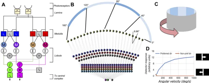
Fig 1. The motion detection section of the model for one eye. A shows the structure of a detector unit spanning two neighbouring
ommatidia, with purple and green outputs responding to angular velocity (AV) in the progressive and regressive directions respectively. M denotes multiplication, / denotes division, the∑denotes summation over the entire eye. Theτare the time constants of leaky integrators. B shows the horizontal layout of the units and connections for a single eye, and the mapping from visual space to the model photoreceptors, with 0˚ representing directly in front of the modelled fly. C shows a diagram of the visual environment, which can be rotated. D shows the response of the angular velocity detector to a single 11.5˚ bar moving across the field of view at different angular velocities. The parameters of the model are (full details can be found in [24]):τ1= 5ms,τ2= 15ms,τb= 1ms,τS= 10ms, and control the range and nature of the angular
increasing AV with a log-linear response as is found in electrophysiological recordings from
the honeybee [21,24]. This motion detector provides the input to the ring attractor both using
the output of the AVDUs to drive changes based on the motion of the environment, but also by summation over smaller regions of the visual field to provide landmark responses.
Ellipsoid body ring attractor network
Recent work has shown that the population activity of the EBw.s neurons in the ellipsoid body
show dynamics and behaviour suggestive of a ring attractor network [11,13]. A ring attractor
is a form of linear attractor network where the connections loop across the two open ends to
form a closed loop. Input due to the all-to-all inhibitory connectivity (Ir) and input due to the
local approximately Gaussian distributed excitatory connectivity (Er
i) ensure a single bump of
activity in the network. We chose a value for the Gaussian excitatory connectivity to match
the bump full value half width (FVHW) measured by Seelig and Jayaraman [11]. The FVHW
measured over 120s of simulation for our model are as follows (experimental values from [11]
in brackets): single bar stimulus 82.7˚±10.7˚ (82.3˚±11.5˚), panorama stimulus 85.8˚±9.5˚ (84.9˚±12.6˚).
The ellipsoid body inDrosophilaconsists of a ring divided radially into 16 regions described
aswedges, and we model each wedge as containing a single neuron of the ring attractor. This
results in connectivity as shown inFig 2.
The activity of this model is driven in two ways, as described in previous work using ring attractors to model vertebrate direction cells (e.g. [29–33]). The first is positional with an input corresponding to a region of the visual field for each wedge. The second is by the time derivative of position: the motion of the visual scene. For the former we only require input directly into the ring attractor however for the latter we must include additional neural cir-cuitry. For the attractor to respond to motion we need two additional neuron types at each wedge location; one for clockwise rotations and one for anticlockwise rotations. These neurons take input from one wedge then output to the neighbouring wedge in the required motion direction. If these neurons have their activity gated multiplicatively by a global driver signal then the bump of activity on the ring will move in each direction in proportion to the strength of the driver signal for that direction. We describe the activity of neurons in the ring, clockwise rotation circuit, and anticlockwise rotation circuit asri,ciandairespectively for each wedgei
up toimax. The positional inputs to the ring arepi(See Eqs (3) and (4) for the static and plastic
versions of this input) weighted by a global factorwp, and the clockwise and anticlockwise
driver signals aredcandda. This gives the dynamics of the ring as:
dri
dt ¼
riþEriþIrþwppiþci 1þaiþ1
tr ð1Þ
Er
i ¼0:6riþ0:35ðrðiþ1Þmodimaxþrði 1ÞmodimaxÞ þ0:225ðrðiþ2Þmodimaxþrði 2ÞmodimaxÞ ð2Þ
Ir¼ 0:1X
imax
0 ri
ai ¼dari
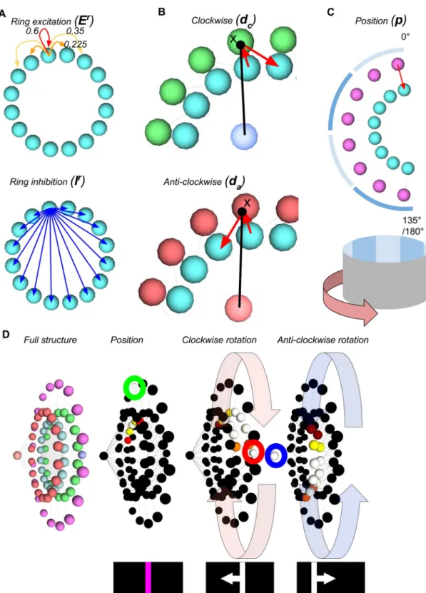
Fig 2. The ring attractor circuit. The components are as follows: Cyan: ring attractor neurons; Green: clockwise
motion rotational neuron (with dark blue driver neuron); Red: anti-clockwise rotational neurons (with pale red driver neuron); Pink: Positional inputs. A shows the connectivity within the ring attractor for a single wedge, with local excitatory connections that decrease with distance, and uniform inhibitory connections. B shows the neural circuits for rotating the bump of activity around the ring clockwise and anti-clockwise for a single pair of wedges. The activity is gated by a single driver neuron (centre of the ring) which multiplies the ring activity to produce the output to the next wedge. C shows the positional input to one half of the ring for one neuron, and the angular mapping to the environment.
The speed with which activity in the ring responds to the driver signals is determined by
the time constant of the ring neurons,τr, which is chosen as 1ms. The numbers in the
equa-tion forEr
i(Eq (2)) describe the weights of the approximate Gaussian distributed excitatory
connections.
Connections between motion detector and ring attractor
The ring attractor is driven by activity from the motion detector in two ways. First motion is
summed across the entire field of view and forms clockwise and anti-clockwise drivers (dcand
da) of the ring attractor. These drivers combine the AVDU outputs in the progressive and
regressive directions across both eyes (pgR,rgR,pgLandrgL) to form signals for leftward and
rightward rotational motion. The driver signals are then multiplicatively (for mechanism see
Nezis et al 2011 [34]) combined with the neighbouring ring attractor activity in a leaky
integra-tor with time constantτy= 0.1mssuch that:
ddc
dt ¼
dcþpgRþrgL
ty
dda dt ¼
daþpgLþrgR
ty
Secondly, the ring attractor is driven by positional information. This information is derived from wide receptive fields evenly spaced across the horizontal field of view. These are designed
to mimic the scale of receptive fields known to exist inDrosophilaCX R4d ring neurons [14].
We use receptive fields, symmetric across the eyes, defined for each eye (Left andRight) by
horizontal neuron ranges (with implicit summation down vertical columns)xkand fixed
weights, which divide the eye into a vertical set of stripes each with a three ommatidia width:
RFjfL;Rg¼
X3kþ2
k¼3k
xk:j¼0 : 7
These receptive fields are connected to the ring attractor retinotopically for the fixed weight
experiments, as shown inFig 2, with a global weighting factorwpvia positional cells. We fix
the weights for the initial experiments to investigate the interactions of the motion and posi-tional signals as well as the behaviour of the neural compass with each individually. These experiments provide context for the plastic weight experiments. They are governed by the
fol-lowing equation with time constantτp= 10ms:
dpi
dt ¼
ð piþRFLiÞ=tp :i<imax=2
ð piþRFRimax=2 iÞ=tp :iimax=2
ð3Þ
8 <
:
Fixed RFs provide a suitable method for driving the compass however they do not agree
with the experimental data of Seelig and Jayaraman [11]. Here we present a model
hypothesis-ing that RFs can be mapped onto compass positions in the EB rhypothesis-ing attractor via plasticity. We
then will test this model with the stimuli presented to the realDrosophila, where the accuracy
the clockwise driver neuron (red) rotating the bump around the ring; the anti-clockwise driver neuron (blue) rotating the bump back to the initial location.
of the neural compass differed depending on the nature of the stimuli, to see if our model pres-ents the same deficits as the real flies do.
To match the proportions of inhibitory and excitatory neurotransmitters in the neurons projecting to the EB, where there are many neurons that are stained for the presence of GABA but fewer for excitatory neurotransmitters, we propose a ‘winner-takes-all’ structure to the input landmark fields. In this each landmark provides inhibitory connections to the other landmarks and excitatory plastic connections to all the EB.ws ring attractor neurons. The
out-puts of the excitatory landmark neuronspiare therefore modelled as follows, where the action
of the inhibitory neurons is subsumed as a summed inhibitory input applied in the EB ring and neuron activation is always positive.
dpl
dt ¼
ð plþRFlL 10
P
m2½m6¼lpmÞ=tp :l<lmax=2 ð plþRFR
lmax=2 l 10 P
m2½m6¼lpmÞ=tp :llmax=2
ð4Þ
(
A Hebbian learning rule with rapid presynaptic weight normalisation [35] is used to learn a
mapping between the landmarks and the ring neurons. The learning rule is also driven by a ‘consolidation’ process where the difference between the sum of the presynaptic weights
(which is normalised to a constant,θ) and the individual weight drives learning alongside the
Hebbian learning by setting the threshold between term depression (LTD) and long-term potentiation (LTP) regimes. This consolidation is required as we seek to bind the marks to activity in the ring attractor that is not initially generated by the output of the
land-mark neurons, and standard Hebbian rules fail in these conditions [36,37]. We will investigate
two boundary conditions of this rule: one where the rate of the consolidation process is twice the rate of the Hebbian process and one where it is half.
These excitatory landmark neurons are then connected to the EB.ws neurons by plastic
weightswliwhich vary according to the rule:
y¼ X m¼imax
m¼0
wml ¼1:0
dwil
dt ¼
0 :wil0
aplðri bðy gwilÞÞ :wil>0
(
whereiis the postsynaptic index,lis the presynaptic index,α= 0.002 is the global learning
rate,β= [0.5, 2] is the consolidation learning factor,γ= 1.1 is the stability of learned weights,
andβ(θ−γwil) sets the LTP/LTD threshold. These weights are then multiplied by the global
landmark weightwp= 0.02.
Methods
Basic attractor responses (Experiments 1 & 2). To test the basic response of the ring
attractor we investigate the behaviour when driven by motion, position, and a combination of the two. This allows us to look at the accuracy of the individual systems, and the accuracy when they are combined. In addition, we can look at the accuracy that different numbers of positional RFs provide, which will provide context when investigating the accuracy of the model in Experiment 3, where plasticity is involved in the positional pathway.
For the initial experiments we use theRFreceptive fields withwp= 0.1 for position only,
andwp= 0.01 for position and motion, as in the absence of a motion signal a greater positional
Since our model will not generate its own turning movements for this set of experiments
we drive the movement of the model using a temporally smoothed (time constantτϕ= 100ms)
summed Gaussian, random, processN(x¼0,σ2= 10), where the change in absolute
horizon-tal rotation (yaw, or azimuthal rotation), of the model,ϕis given by:
dN
dt ¼Nð0;10Þ
d
dt ¼
þN
tAz
To compare the model ring attractor representation of azimuthal rotation with the simu-lated azimuthal rotation we take a vector average of the activity of the ring attractor. We weight
the vector formed from the centre of the ring to each neuron’s location in the ring (vi) by that
neuron’s activity (ri) and sum the vectors to give a resultant direction vsum. We then take the
estimated azimuth angle,ϕest, from this vector to the initial forward direction vinitand account
for prior complete rotations by counting the transitions past 180˚ (Ntrans).
vsum¼
Ximax
i¼0 rivi
est ¼ arccosð^vsumv^initÞ þ2pNtrans
We present a black environment with a single grey bar. The bar subtends 11.5˚ of visual angle in the horizontal direction, has infinite extent in the vertical direction, and has a lumi-nance of 0.8 out of a maximum of 1.0. The model controls the azimuthal rotation of a virtual insect within this environment with fixed location. This mimics the environment presented to
restrained behavingDrosophilain experiments [11]. The field of view of the model insect is
described in the section ‘Motion detection’.
We process the data to compute the circular mean and standard deviation of the difference between the estimated and simulated azimuthal rotations using the Matlab Circular Statistics
Toolbox [38]. As there is a processing delay in the ring attractor responding to changes in the
azimuth of the simulated insect we calculate the standard deviation using offsets in the data from 0 to 60ms in 1ms increments, and use the offset with the minimum standard deviation.
Learned landmark attractor responses (Experiment 3). This experiment investigates
the way in which the motion and position pathways interact when the positional information must be learned. This motivation for this version of the model arises from the experimental
evidence in Seelig and Jayaraman [11] that the activity in EB.w.s neurons has an angular offset
to the position of the landmarks on the visual field which can change over long time periods for a single fly. This evidence indicates that the positional RFs do not map linearly onto the ring attractor but that the mapping may be plastic. We choose two parameterisations of the learning rule, and these affect the speed of the consolidation part of the learning rule (see Sec-tionLandmark learning) but not the Hebbian learning part of the rule. One parameterisation reduces the speed of the consolidation process and thus is closer to a pure Hebbian rule where the weights can change their mapping more easily. The other parameterisation increases the speed of consolidation which produces more stable weight mappings that require significant contradictory activity to change.
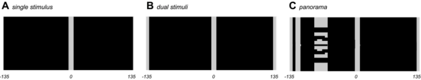
Three stimulus environments were used for this experiment: single bar, dual bar and
pano-rama. These are shown inFig 3. These environments are chosen to replicate the environments
used by Seelig and Jayaraman [11] with only the dual bar experiment exhibiting rotational
symmetry. The ‘models as animals’ protocol is used for this experiment, where identical naïve models are presented with one of the stimulus environments, and the difference in the random walk taken determines the learning that occurs. For Experiment 3 simulations are 60s long, with 10s given for learning to occur, and performance analysis being presented for the follow-ing 50s. The simulation timestep is 0.1ms.
Statistical analyses. Correlation: Correlation analyses were performed using Pearson’s
test, as used in Seelig and Jayaraman’s analysis [11] in GNU Octave using thecorr()
com-mand [39].
Non-parametric multi-sample test: non-parametric multi-sample test analyses were
per-formed using the Matlab Circular Statistics Toolbox [38] functioncirc_cmtest(). For
comparing between two simulation runs in Experiment 1 the difference between the actual azi-muth and the ring attractor aziazi-muth was calculated for each time point, and time points were sampled at 100ms intervals to provide independent samples for analysis. For analysis between stimuli in Experiment 3 the set of standard deviations of all simulation runs for a stimulus were taken as the independent variable sets.
Clustering: The distribution of the weights from the RFs to the ring attractor were analysed using clustering. The weights from each RF to the ring attractor neurons were taken as vectors with direction denoted by the target ring attractor neuron and magnitude denoted by the weight. These vectors for each RF were then averaged to give the resultant preferred direction for that RF. The direction of each RF was then subtracted from the direction that RF would map to if the RFs were arranged in an even retinotopic mapping: thus RF directions corre-sponding to a single retinotopic mapping would now have similar directions after subtraction. All RF vectors were then next set to unit length, and decomposed into cosine and sine compo-nents. These components were then clustered using 2D clustering via the DBSCAN algorithm
implementation from Scikit-learn [40] with= 0.25.
Results
Experiment 1: The activity in the ring attractor tracks rotation of a single
moving bar with greater accuracy if position and motion are combined
We ran the model for 120s (at 0.1ms timesteps) of simulation time for three conditions:
motion input to the ring attractor only; position input usingRFreceptive fields to the ring
attractor only; combined motion and position input, with the position input reduced tenfold so it does not dominate.
Fig 3. Stimuli for the model. A Single stimulus. B Dual stimuli. C Panorama of stimuli. These stimuli are based on the angular dimensions
Fig 4shows the azimuthal rotation estimated by the model ring attractor and the actual azi-muthal rotation of the virtual insect, for each of these conditions. In addition the mean and standard error of the difference between the two azimuth values is shown. The Pearson’s
corre-lation between the two azimuthal rotation measures is high (R>0.97) in all conditions. There
is a clear improvement in the correspondence between the two azimuth values when position cues are used, and even greater improvement when position and motion are combined. It should be noted, however, that the improvement of motion and position over position alone is small. A non-parametric multi-sample test (see Methods for details) shows that all differences in the distributions of the difference between the ring attractor azimuth and actual azimuth
between conditions are statistically significant (allp0.01 except position: motion and
posi-tion (p<0.05)).
Experiment 2: More positional receptive fields provide more accurate
tracking of the bar location
To test the influence that the number of receptive fields have on the performance of the track-ing accuracy of the rtrack-ing attractor we ran the model with differtrack-ing numbers of receptive fields. This was performed by removing an evenly spaced proportion of the receptive fields, by halv-ing the number of fields, by providhalv-ing one eighth the number of fields, or in the final case by only providing one receptive field. The paradigm otherwise remained identical to that in
Experiment 1.Fig 5shows the results of these experiments. It can be seen that there is a
decrease in accuracy as the number of receptive fields decreases however even one receptive field provides much greater accuracy than when no receptive fields (i.e. motion input only) are used. A non-parametric multi-sample test (see Methods for details) shows that all differences
are highly statistically significant due to the size of the data set (p0.01). The Pearson’s
correlation between the two azimuthal rotation measures is high (R>0.99) in all conditions.
Fig 4. Ring attractor azimuth estimate accuracy. A shows the simulated (blue) and estimated (grey) azimuthal rotations when the ring
attractor is driven only by the motion of the bar. There is overall good tracking for much of the simulation however there are time periods where the estimate drifts away from the simulated value. B show the same rotations when positional cues drive the ring attractor. There is better tracking, however D shows that the width of the receptive fields leads to a stepped profile for the ring attractor estimate as movement of the bar within a receptive field cannot be detected. C shows the same rotations with combined position and motion driving the ring attractor. There is good tracking, and E shows that the motion signal can compensate for the insensitivity of the motion system within a receptive field. F summarises the results showing that the circular mean and standard deviation (calculated using the Matlab Circular Statistics Toolbox [38]) of the difference between the simulated and estimated rotations is largest with motion only driving the ring attractor and smallest with combined motion and position.
Experiment 3: A Hebbian rule allows learning of the mapping of
landmarks to the ring attractor
We next tested the ability of our Hebbian based learning rule to associate the position of land-marks in the visual world with positions on the neural compass with two parameter variants,
chosen by a limited exploration of the parameter space for the rate of weight consolidation,β.
The two parameterisations show two distinct modes of learning for the model, one that creates
a retinotopic mapping that can change once established (β= 0.5) and one which creates a fixed
retinotopic mapping (β= 2.0). These values are chosen as examples as more extreme values of
βfail to create retinotopic mappings and match the experimental data. The stimuli used to test
the model were replications of those used by Seelig and Jayaraman [11], consisting of a single
bright vertical bar on a dark background, two bars separated by 135˚ horizontally (thus dis-playing 2-fold rotational symmetry in the 270˚ visual world), and a panorama of four bars with
no rotational symmetry, as shown inFig 3.
Figs6&7shows the results for all these three cases for each parameterisation, with
exam-ples showing the time evolution of the landmark weights, and the circular mean and standard deviation for the final 50s of the 60s simulation. Interestingly, despite the marked differences in the evolution of the weights, a non-parametric multi-sample test (see methods for details)
shows low or no significance in the difference (p>0.07, except dual bar (p0.1)) between
the distributions of standard deviations for the two values ofβ. There are, however, significant
differences between the distributions of standard deviations for the different stimuli in both
cases (allp0.01). The Pearson’s correlation between the two azimuthal rotation measures is
high (R>0.99) in all conditions. In keeping with the results from Experiment 2, Pearson’s
cor-relation analysis of change in tracking error and the absolute azimuthal position showed no significant correlation between these data for any simulation run.
Parameter variant 1:β= 0.5. With a purer Hebbian form of learning we see that only in
the case of the single bar stimulus set does the model maintain weight mapping, and there is variation even in this mapping over time. With the panorama stimuli the model changes between mappings throughout the trial (evidenced by the opposing green and purple at fixed radial distances). The model does maintain a fixed offset between the ring attractor direction and the world rotation in almost all cases, but this is driven by the changing weight mappings.
Fig 5. Receptive field number correlates with tracking accuracy in the ring attractor. A Greater numbers of receptive fields provide a
reduction in the circular standard deviation (calculated using the Matlab Circular Statistics Toolbox [38]) of the error between the actual azimuth and the estimate from the ring attractor. B The correlation between the change in the tracking error and the change in azimuth shows significant positive correlation, which is significantly different for larger RF numbers than for smaller RF numbers. C The correlation between the change in tracking error and the absolute azimuth shows no significant correlation (see main text for details of the test). D An example of the correlation between the change in tracking error and the change in azimuth (for 16 RF, data sampled every 1000 iterations, using the temporal offset calculated to find the mean azimuthal offset). The colour of each point indicates the absolute azimuth, showing no correlation to error change. One example is used as it is representative of all such plots.
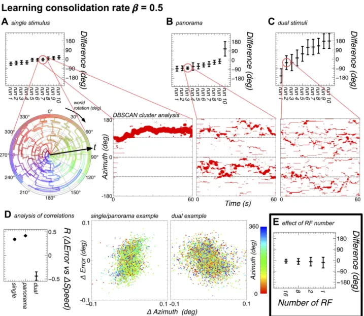
Fig 6. The model can learn to map landmarks to positions on the ring attractor with slow consolidation (β= 0.5) of the plastic weights. In addition the evolved offsets when the ring attractor is seeded to one position are shown. A The model performance (see E for comparison with the results from Experiment 2) in terms of mean and circular standard deviation (calculated using the Matlab Circular
Statistics Toolbox [38]) of the ring attractor direction from the world direction (corresponding to the location of the single stimulus, and remapped from 270˚ to 360˚) is shown at the top, and shows that the model is able to track the motion of the world well in all cases, with an offset to the position of the stimulus on the visual field. Additionally, a polar plot contains an example of the evolution of the weights over the course of the simulation (with time increasing from the centre to the outside) for a single stimulus. In the polar plot each receptive field (RF) is given a colour, with the key around the outside of the ring, and the angular position of each line denotes the position on the ring attractor that each RF maps to. An ordered mapping, with no offset, should therefore be shown by each line lying in the circular segment under the corresponding key item. Instead, we see that the weights remap the 260˚ world onto approximately 360˚ of the ring attractor, and the learning is established early in the simulation, although the weights do show changes in the mapping over the course of the simulation. A second Cartesian plot shows the clustering of the RFs into retinotopic maps (see Methods for details), with the size of the marker denoting the number of RFs in a cluster. For the single stimulus it can be seen that a single map evolves, but changes offset over time. B As A, but with the panorama. The polar plots are not helpful for the panorama as there are multiple retinotopic mappings developed. Here there is once again a good performance in tracking the world in most cases, albeit with one run where tracking performance is poor. The example showing the weight clustering shows that multiple retinotopic mappings are developed, however these mappings change over the course of the simulation. C As A, but with dual stimuli. In this case the model exhibits poor performance tracking the world, and the weights remain largely changeable throughout the simulation. D This panel shows the correlations between the changes in azimuthal position and the changes in the offset between the actual azimuth and the azimuth represented on the ring attractor. The single and panorama simulations show a similar correlation to that found with fixed RFs, however the dual stimuli simulations show a negative correlation between the change in position and the change in error.
In the case of the dual stimuli the model forms a rough and extremely variable mapping, and the neural compass ‘transitioning’ between the stimuli degrades the performance.
Parameter variant 2:β= 2.0. This variant of the learning rule forms more stable weight
mappings, and this is clear from the polar weight plots. In all cases for the single bar and pano-rama stimuli sets it is clear that the model is able to learn stable weight mappings, albeit with a fixed offset between the neural compass and the visual stimuli. There is a notable difference
Fig 7. The model can learn to map landmarks to positions on the ring attractor with fast consolidation (β= 2.0) of the plastic weights. In addition the evolved offsets when the ring attractor is seeded randomly are shown. A AsFig 6: A except withβ= 2.0. Here the weights finish evolving early on in the simulation and remain fixed after that point. There is only one retinotopic mapping developed.
B AsFig 6: B except withβ= 2.0. The weights form three retinotopic mappings, which persist for the rest of the simulation. C AsFig 6: C except withβ= 2.0. The weights form many weak mappings, with few RFs belonging to any one mapping. D This panel shows ‘transitioning’ between stimuli as found in the experimental data of Seelig and Jayaraman [11]. E This panel shows the correlations between the changes in azimuthal position and the changes in the offset between the actual azimuth and the azimuth represented on the ring attractor. The single and panorama simulations show a similar correlation to that found with fixed RFs, however the dual stimuli simulations show a negative correlation between the change in position and the change in error.
between the mapping learned in the single stimulus case and that learned from the panorama stimuli. The single stimulus rapidly produces a clear mapping, which does not alter after the first few seconds. The panorama stimuli show less specificity, with some RFs mapping to dif-ferent offsets of the panorama relative to the model head direction.
In the case of the two bar stimuli, there is weaker tracking, and an analysis of the individual trials shows that this is in part due to the neural compass ‘transitioning’ between tracking each of the two bars in the environment. This is consistent with the behaviour found by Seelig and
Jayaraman [11]. The cluster weight plot shows a very non-topographic global mapping, due to
many different mappings being laid over each other. These mappings are, however, fixed for most of the simulation and therefore the source of the ‘transitioning’ is not due to changes in weights. The angular distance between the mappings indicates that one source of the transi-tions could be the bump activity transitioning between being driven by each of two different mappings, however it should also be noted that transitioning can also be caused by a given mapping moving from tracking one stimulus to tracking the other stimulus. Analysis of the distribution of the offset between the actual azimuth and ring attractor azimuth does not resolve this ambiguity.
Discussion
The central complex in insects is an intriguing structure, which is only beginning to be
under-stood. Centrally positioned, ancient [41] and the source of massive sensory convergence, it is
well placed to perform a range of tasks. It is therefore not surprising that it has been implicated
as having a role in locomotion [4], courtship [2], visual pattern memory [6] and polarisation
detection [8]. We present a model here that frames what we do know about the central
com-plex, that it is the site of activity that tracks the heading of the insect, and we investigate the computational mechanisms behind this activity and provide mechanistic explanations for fea-tures of the experimental data that were previously not understood. While this study does not provide a conclusive summary of the role of the central complex, it provides the basis for more elaborate models.
Previous modelling work investigating head position cells in vertebrates, notably the rat, has mainly focused on the self organisation of ring attractor networks based on associative learning rules (e.g. [30–33]), which is not a concern in the insect as there is a well established
morphology that contains the connections required for a ring attractor [42]. Learning of
land-marks is mentioned, but not computationally evaluated [29]. We therefore present a model
that does not focus on the dynamics of the ring attractor, but instead on the signals that drive it and their association with landmarks in the visual world.
It is notable that the performance of the model in the single stimulus trials is equivalent to the performance of the fixed RF model with 16 RFs for both learning rule parameterisations. This shows that fixed RFs provide less flexibility for equivalent performance.
Another key point is that there is still a spread of offsets between the neural compass and the real world landmarks found in the model behaviour when the ring attractor is seeded with activity at a fixed position: demonstrating that there is no implicit fixed bias to the offset induced by the starting state of the ring attractor.
The two parameterisations of the learning rule show similar behaviour of the neural com-pass but very different outcomes in the evolution of the plastic weights over the simulation.
This shows that there are a range of parameter values forβ, the consolidation speed, that can
reproduce the experimental findings. To separate the likelihood of these two values ofβbeing
[7] then the weights must be resistant to change, so for such a role we favour the hypothesis
that the real mechanism will be closer to the model withβ= 2.0.
Finally, and most importantly, the role of the motion signal becomes clear when landmark learning is considered. Previously we have seen that the motion signal provides a poor substi-tute for positional information, accumulating errors rapidly. In addition the motion signal provides little increase in accuracy over a purely positional system. The model therefore pre-dicts that these are not the reasons for a motion signal in the CX. The model instead prepre-dicts that the motion signal provides a required training signal when the landmarks are being learned, allowing neighbouring landmarks to trigger neighbouring neurons in the neural com-pass, as the activity in the ring attractor is driven initially by motion only. This explains the existence of the two systems, as motion cannot represent direction without drift, but absolute direction cannot be learned without the motion signal.
In summary, our model makes the following predictions of several features found in the experimental data.
1. Few receptive fields (RF) are required for accurate tracking of rotation, and the number of RFs required for good rotation tracking aligns with the numbers of visual neurons converg-ing on the central complex in the fly [14,43].
2. As found in the data, dual stimuli will result in poor performance, and that ‘transitioning’ will occur between tracking each of the stimuli.
3. There will be a range of offsets between the location of the stimuli on the visual field and the neural compass, and that the 270˚ arena is mapped onto the full ring attractor.
4. Finally, our model predicts that rotational, non-positional information is present in the central complex because it is an essential part of the process of learning how to associate RFs with compass directions. It is not to provide a backup form of rotation tracking (as it accumulates errors rapidly), or to improve tracking with a learned positional mapping (as the improvement it provides is small).
We acknowledge that the current study has limitations. One is that, in the absence of motion activity, the activity in the ring attractor is drawn to stable states centred on the neurons in the ring attractor circle. Since there are only 16 neurons in our attractor, this means that inaccuracies can accrue rapidly. When driven with a random Gaussian process these inaccuracies average out over the course of the simulation, however when driven by more purposeful behaviour they can significantly affect the behaviour of our model. It is possible that a more complex ring attractor could be devised that does not suffer from these stable states. Additionally some aspects of model behaviour are difficult to compare to the experimental data. For example, Seelig and Jayaraman compute the correlation between the angle indicated in the central complex and the heading of the fly, and find that there is a variability in correlation between runs. In our model the correlation is always extremely
high (R>0.99), and it is uncertain whether this difference is due to noise introduced by
the recording mechanism used by Seelig and Jayaraman, or differences between the model and the biological system. A similar argument also applies where we do not find more than one activity bump on the ring attractor at any point, while Seelig and Jayaraman occasion-ally do.
Does the central complex contain a compass or not? The model indicates that it is necessary with the simple learning shown here to bind direction to the angular position of a single
signif-icant feature in the environment. This means that as thein silicoanimal moves around, the
‘compass’ is not a compass in the sense we mean but more akin to a magnetic compass near the poles: it points to a single significant feature in the current environment. This is a change in the role of the ring attractor, but for simple environmental associative learning does not remove the usefulness of the system. For example, so long as the ring attractor is consistent in direction for a given environment, and given an additional means of determining location based on multiple sensory features, a mechanism driving behaviour towards a rewarded head-ing will still be useful. Such a mechanism allows that the ‘compass’ is local but requires a posi-tional system (or place memory) to work in combination with.
The absence of a global compass does constrain certain behaviours found in insects, notably long range scouting and navigation, which require a form of path integration. It is therefore interesting to note that honeybees only forage at previously visited locations close to home
under cloudy skies [44] when absolute direction information from UV light polarisation is not
available to them. Such behaviour does suggest that a local compass, as found here, may be
suf-ficient for place-based navigation as is found inDrosophilaand provides an avenue for better
understanding such behaviours.
The existence of the compass, and the understanding of how it is implemented, provided a first step in understanding the central complex, and this work adds to complementary studies that unearth the possible computational mechanisms at play in the central complex (path inte-gration [3,45], the celestial compass [9], and place finding [7] for example).
The possibilities unleashed by understanding the CX far exceed an understanding of brain function in insects. Such understanding may also ultimately lead to the development of algo-rithms for advanced robotic autonomy: giving robots the ability to rapidly orient themselves within a new environment and associate headings relative to landmarks with behavioural out-comes. This ability would permit goal directed behaviour with greater autonomy than is
cur-rently possible and, given the abilities of more advanced insects (notablyHymenoptera) to
navigate over long distances, would provide the basis for the development of more advanced navigation.
Author Contributions
Conceptualization: AC AB.
Data curation: AC.
Formal analysis: AC.
Funding acquisition: JM AB.
Investigation: AC.
Methodology: AC EV.
Project administration: JM.
Software: AC.
Supervision: JM AB.
Visualization: AC.
Writing – original draft: AC.
References
1. Utting M, Agricola H, Sandeman R, Sandeman D. Central complex in the brain of crayfish and its possi-ble homology with that of insects. J Comp Neurol. 2000; 416(2):245–61. doi:10.1002/(SICI)1096-9861 (20000110)416:2%3C245::AID-CNE9%3E3.3.CO;2-1PMID:10581469
2. Homberg U. Evolution of the central complex in the arthropod brain with respect to the visual system. Arthropod Struct Dev. 2008; 37(5):347–62. doi:10.1016/j.asd.2008.01.008PMID:18502176
3. Wessnitzer J, Webb B. Multimodal sensory integration in insects—towards insect brain control architec-tures. Bioinspir Biomim. 2006; 1(3):63–75. PMID:17671308
4. Strauss R. The central complex and the genetic dissection of locomotor behaviour. Curr Opin Neurobiol. 2002; 12(6):633–638. doi:10.1016/S0959-4388(02)00385-9PMID:12490252
5. Kathman ND, Kesavan M, Ritzmann RE. Encoding wide-field motion and direction in the central com-plex of the cockroach Blaberus discoidalis. J Exp Biol. 2014; 217(22). doi:10.1242/jeb.112391PMID: 25278467
6. Wang Z, Pan Y, Li W, Jiang H, Chatzimanolis L, Chang J, et al. Visual pattern memory requires foraging function in the central complex of Drosophila. Learn Mem. 2008; 15(3):133–42. doi:10.1101/lm.873008 PMID:18310460
7. Ofstad TA, Zuker CS, Reiser MB. Visual place learning in Drosophila melanogaster. Nature. 2011; 474 (7350):204–7. doi:10.1038/nature10131PMID:21654803
8. Labhart T, Meyer EP. Neural mechanisms in insect navigation: polarization compass and odometer. Curr Opin Neurobiol. 2002; 12(6):707–714. doi:10.1016/S0959-4388(02)00384-7PMID:12490263
9. Homberg U, Heinze S, Pfeiffer K, Kinoshita M, el Jundi B. Central neural coding of sky polarization in insects. Philos Trans R Soc London B Biol Sci. 2011; 366 (1565). doi:10.1098/rstb.2010.0199PMID: 21282171
10. Taube J, Muller R, Ranck J JB. Head-direction cells recorded from the postsubiculum in freely moving rats. I. Description and quantitative analysis. J Neurosci. 1990; 10(2):420–435. PMID:2303851
11. Seelig JD, Jayaraman V. Neural dynamics for landmark orientation and angular path integration. Nature. 2015; 521(7551):186–191. doi:10.1038/nature14446PMID:25971509
12. Varga AG, Ritzmann RE, Taube JS, Muller RU, Ranck JB, Taube JS, et al. Cellular Basis of Head Direc-tion and Contextual Cues in the Insect Brain. Curr Biol. 2016; 26(14):1816–28. doi:10.1016/j.cub.2016. 05.037PMID:27397888
13. Turner-Evans DB, Jayaraman V, elAˆ Jundi B, Warrant EJ, Byrne MJ, Khaldy L, et al. The insect central complex. Curr Biol. 2016; 26(11):R453–7. doi:10.1016/j.cub.2016.04.006PMID:27269718
14. Seelig JD, Jayaraman V. Feature detection and orientation tuning in the Drosophila central complex. Nature. 2013; 503(7475):262–6. doi:10.1038/nature12601PMID:24107996
15. Wolf R, Heisenberg M. Visual control of straight flight in Drosophila melanogaster. J Comp Physiol A. 1990; 167(2):269–83. doi:10.1007/BF00188119PMID:2120434
16. Dill M, Wolf R, Heisenberg M. Behavioral analysis of Drosophila landmark learning in the flight simula-tor. Learn Mem. 1995; 2(3–4):152–60. doi:10.1101/lm.2.3-4.152PMID:10467572
17. Wolf R, Heisenberg M. Visual space from visual motion: turn integration in tethered flying Drosophila. Learn Mem. 1997; 4(4):318–27. doi:10.1101/lm.4.4.318PMID:10706369
18. Guo C, Du Y, Yuan D, Li M, Gong H, Gong Z, et al. A conditioned visual orientation requires the ellipsoid body in Drosophila. Learn Mem. 2014; 22(1):56–63. doi:10.1101/lm.036863.114PMID:25512578
19. McCann GD, MacGinitie GF. Optomotor Response Studies of Insect Vision. Proc R Soc B Biol Sci. 1965; 163(992):369–401. doi:10.1098/rspb.1965.0074
20. Kirchner WH, Srinivasan MV. Freely flying honeybees use image motion to estimate object distance. Naturwissenschaften. 1989; 76(6):281–282. doi:10.1007/BF00368643
21. Ibbotson MR. Evidence for velocity-tuned motion-sensitive descending neurons in the honeybee. Proc R Soc L [Biol]. 2001; 268(1482):2195–201. doi:10.1098/rspb.2001.1770
22. Barron A, Srinivasan MV. Visual regulation of ground speed and headwind compensation in freely flying honey bees (Apis mellifera L.). J Exp Biol. 2006; 209(Pt 5):978–84. doi:10.1242/jeb.02085PMID: 16481586
23. Fry SN, Rohrseitz N, Straw AD, Dickinson MH. Visual control of flight speed in Drosophila melanoga-ster. J Exp Biol. 2009; 212(Pt 8):1120–30. doi:10.1242/jeb.020768PMID:19329746
25. Pfeiffer K, Homberg U. Organization and functional roles of the central complex in the insect brain. Annu Rev Entomol. 2014; 59:165–84. doi:10.1146/annurev-ento-011613-162031PMID:24160424
26. Richmond P, Cope A, Gurney K, Allerton DJ. From model specification to simulation of biologically con-strained networks of spiking neurons. Neuroinformatics. 2013; 12(2):307–23. doi: 10.1007/s12021-013-9208-z
27. Cope AJ, Richmond P, James SS, Gurney K, Allerton DJ. SpineCreator: A graphical user interface for the creation of layered neural models. In-press. 2015;
28. Power ME. The effect of reduction in numbers of ommatidia upon the brain of Drosophila melanogaster. J Exp Zool. 1943; 94(1):33–71. doi:10.1002/jez.1400940103
29. Skaggs WE, Knierim JJ, Kudrimoti HS, McNaughton BL. A Model of the Neural Basis of the Rat\text-quotesingle s Sense of Direction. In: Tesauro G, Touretzky DS, Leen TK, editors. Adv. Neural Inf. Pro-cess. Syst. 7. MIT Press; 1995. p. 173–180. Available from: http://papers.nips.cc/paper/890-a-model-of-the-neural-basis-of-the-rats-sense-of-direction.pdf.
30. Xie X, Hahnloser RHR, Seung HS. Double-ring network model of the head-direction system. Phys Rev E. 2002; 66(4):041902. doi:10.1103/PhysRevE.66.041902
31. Stringer SM, Trappenberg TP, Rolls ET. Self-organizing continuous attractor networks and path integra-tion: one-dimensional models of head direction cells. Comput Neural Syst. 2002; 13:217–242.
32. Stringer SM, Rolls ET, Trappenberg TP. Self-organizing continuous attractor network models of hippo-campal spatial view cells. Neurobiol Learn Mem. 2005; 83(1):79–92. doi:10.1016/j.nlm.2004.08.003 PMID:15607692
33. Knierim JJ, Zhang K. Attractor Dynamics of Spatially Correlated Neural Activity in the Limbic System HD: head direction. Annu Rev Neurosci. 2012; 35:267–85. doi: 10.1146/annurev-neuro-062111-150351
34. Nezis P, van Rossum MCW. Accurate multiplication with noisy spiking neurons. J Neural Eng. 2011; 8 (3):034005. PMID:21572218
35. Zenke F, Gerstner W. Cooperation across timescales between and Hebbian and homeostatic plasticity. Philos Trans R Soc London, Ser B Biol Sci. 2016; (preprint).
36. Vasilaki E, Fre´maux N, Urbanczik R, Senn W, Gerstner W. Spike-Based Reinforcement Learning in Continuous State and Action Space: When Policy Gradient Methods Fail. PLoS Comput Biol. 2009; 5 (12):e1000586. doi:10.1371/journal.pcbi.1000586PMID:19997492
37. Richmond P, Buesing L, Giugliano M, Vasilaki E. Democratic Population Decisions Result in Robust Policy-Gradient Learning: A Parametric Study with GPU Simulations. PLoS One. 2011; 6(5):e18539. doi:10.1371/journal.pone.0018539PMID:21572529
38. Berens P. CircStat: A MATLAB Toolbox for Circular Statistics; 2009. Available from:http://www. jstatsoft.org/v31/i10/.
39. John W Eaton David Bateman SH, Wehbring R. {GNU Octave} version 4.0.0 manual: a high-level inter-active language for numerical computations; 2015. Available from:http://www.gnu.org/software/octave/ doc/interpreter.
40. Pedregosa F, Varoquaux G, Gramfort A, Michel V, Thirion B, Grisel O, et al. Scikit-learn: Machine Learning in {P}ython. J Mach Learn Res. 2011; 12:2825–2830.
41. Strausfeld NJ, Hirth F. Deep Homology of Arthropod Central Complex and Vertebrate Basal Ganglia. Science (80-). 2013; 340 (6129). doi:10.1126/science.1231828
42. Wolff T, Iyer NA, Rubin GM. Neuroarchitecture and neuroanatomy of the Drosophila central complex: A GAL4-based dissection of protocerebral bridge neurons and circuits. J Comp Neurol. 2015; 523 (7):997–1037. doi:10.1002/cne.23705PMID:25380328
43. Dewar ADM, Wystrach A, Graham P, Philippides A. Navigation-specific neural coding in the visual sys-tem of Drosophila. Biosyssys-tems. 2015; 136:120–7. doi:10.1016/j.biosystems.2015.07.008PMID: 26310914
44. Dyer FC, Gould JL. Honey bee orientation: a backup system for cloudy days. Science. 1981; 214 (4524):1041–2. doi:10.1126/science.214.4524.1041PMID:17808669