This is a repository copy of
Diffusion Wavelet Embedding: a Multi-resolution Approach for
Graph Embedding in Vector Space
.
White Rose Research Online URL for this paper:
http://eprints.whiterose.ac.uk/121724/
Version: Accepted Version
Article:
Bahonar, Hoda, Mirzaei, Abdolreza and Wilson, Richard Charles
orcid.org/0000-0001-7265-3033 (2017) Diffusion Wavelet Embedding: a Multi-resolution
Approach for Graph Embedding in Vector Space. Pattern Recognition. pp. 1-37. ISSN
0031-3203
https://doi.org/10.1016/j.patcog.2017.09.030
[email protected] Reuse
This article is distributed under the terms of the Creative Commons Attribution-NonCommercial-NoDerivs (CC BY-NC-ND) licence. This licence only allows you to download this work and share it with others as long as you credit the authors, but you can’t change the article in any way or use it commercially. More
information and the full terms of the licence here: https://creativecommons.org/licenses/
Takedown
If you consider content in White Rose Research Online to be in breach of UK law, please notify us by
Diffusion Wavelet Embedding: a Multi-resolution
Approach for Graph Embedding in Vector Space
Hoda Bahonara,∗, Abdolreza Mirzaeia, Richard C. Wilsonb
aDept. of Electrical and Computer Engineering, Isfahan University of Technology, Iran b
Dept. of Computer Science, University of York, UK
Abstract
In this article, we propose a multiscale method of embedding a graph into a
vec-tor space using diffusion wavelets. At each scale, we extract a detail subspace
and a corresponding lower-scale approximation subspace to represent the graph.
Representative features are then extracted at each scale to provide a scale-space
description of the graph. The lower-scale is constructed using a super-node
merging strategy based on nearest neighbor or maximum participation and the
new adjacency matrix is generated using vertex identification. This approach
allows the comparison of graphs where the important structural differences may
be present at varying scales. Additionally, this method can improve the
differen-tiating power of the embedded vectors and this property reduces the possibility
of cospectrality typical in spectral methods, substantially. The experimental
re-sults show that augmenting the features of abstract levels to the graph features
increases the graph classification accuracies in different datasets.
Keywords: Spectral graph embedding, diffusion wavelet, multi-resolution
analysis, graph summarization, scale space
1. Introduction
The graph data structure improves the expressiveness of vectors by
describ-ing objects in terms of the relationships between parts. This expressiveness in
∗
Corresponding author
Email addresses: [email protected](Hoda Bahonar),[email protected]
addition to the simplicity of presentation makes them so popular and there is
a rapidly growing interest in representation of different objects by graphs in
5
different fields of science. The graph of covalence relation between chemical
molecules [1], the network of tertiary structure of proteins [2], and the skeleton
of objects in images and videos [3] are some examples of objects represented by
graphs.
The graph structure is determined by an unordered set of edges between
10
an unordered set of nodes. This flexibility is a double-edged sword. On the
one hand, it causes the simplicity of object representation and this simplicity
results in better understanding of the internal relations of the objects. On
the other hand, it makes the procedure of graph handling so time consuming.
Different node permutations result in identical (or isomorphic) graphs, but the
15
checking of this relationship between two graphs is an NP-complete problem [4].
There are some other problems in handling graphs, mentioned in [5, 6, 7, 8],
which motivate researchers to embed graphs in vector space during the last two
decades. Graph embedding in vector space tries to extract the differentiating
graph features and insert them into vectors. These vectors can be processed
20
subsequently through the numerous statistical pattern analysis methods in order
to recognize patterns in corresponding graphs.
Of course some information is lost due to embed the flexible graph structure
into a relatively limited vector structure, but the advantage of the embedded
vectors is that we can utilize the full power of numerous statistical pattern
25
recognition and machine learning techniques. It is crucial therefore that the
embedding method captures as much of the rich graph structure as possible.
Multi-resolution approaches have proved very effective in many areas of pattern
recognition, particularly in image analysis and computer vision, where the
multi-scale representation can pull out important features even when they appear at
30
varying scales. This is the motivation for this paper, where we generate a
multi-resolution embedding of a graph based on the graph diffusion wavelet concept [9].
We anticipate that such a representation will be richer and improve comparison
A scale-based representation is already implicit in a number of graph
em-35
bedding methods, particularly those based on the graph eigendecomposition,
where the eigenvalue, in some sense, reflects the scale of the feature. Several
works in the literature establishes connection between the structural properties
of graphs and the spectral features of their representation matrices [10]. These
attempts are grouped in the field of spectral graph theory and they are used
40
as the feature extraction approach in spectral graph embedding in vector space
[5, 11, 12]. The mentioned spectral features are obtained in polynomial time [13]
from the eigendecomposition of graph, which is stated as follows: A= ΦΛΦ∗,
whereA, Φ and Λ are the representation matrix, the matrix with eigenvectors
on its columns and the diagonal matrix of the eigenvalues, respectively. None
45
of these generate an explicit scale-space representation or can control the scale
of the representation.
The graph spectrum (i.e. the vector of graph eigenvalues) is invariant to
different node permutations and has proved to be a useful graph embedding
method [14]. Unfortunately the problem of cospectrality, i.e. different graphs
50
having the same spectrum, and lack of distinctiveness limits this approach.
Al-most all trees have cospectral mate [15] and there are works to produce
cospec-tral non-isomorphic graphs [16, 17]. This problem can be alleviated by using
eigenvectors [18] but in this approach there is no direct connection to the
struc-tural aspects of the graph.
55
In this article, we try to create a rich graph embedding through a
multi-resolution approach. Structural properties of graphs exist at different scales
within the graph. Two graphs may be similar at one scale while they are
dif-ferent at another scale. For example, consider the comparison of two social
networks. The networks may be different or similar in the communication
be-60
tween individuals (small scale), the structure of the constitutive communities
(intermediate scale), and the overall structure of the network and connections
between communities (large scale). The point at which scales convey the useful
information about the differences/similarities depends on the application. So,
mere extracting features from the initial graph, as it was done in previous works,
does not seem reasonable enough for all the applications.
For multi-resolution embedding proposed in this article, the spectrum of
different levels of approximation and detail are encapsulated into a feature
vec-tor. The mapping of graph into the approximation and detail subspaces is done
through the diffusion wavelet [9]. The summary graph of each level is extracted
70
using this wavelet and some heuristics. This abstract graph1 is utilized as the
input of the diffusion wavelet for the next level. To the best of our
knowl-edge, there is not any application of multi-resolution signal processing methods
into graph embedding. The experimental results show that this approach can
improve the classification accuracy in different applications.
75
In Section 2, some related works are presented. After declaring some basic
concepts in Section 3, the proposed method is described in Section 4. The
experimental results are displayed in Section 5 and finally Section 6 presents
some conclusion remarks and future works.
2. Related work
80
The graph embedding methods can be divided into three groups:
probing-based, prototype-based and spectral methods. In probing-based methods [6, 7],
the frequent features are extracted from the graphs and their frequencies are
embedded into the fixed sized vectors. In prototype-based methods [8, 21], some
special prototypes are selected or made from training graphs and the differences
85
of other graphs to these graphs are encoded into their feature vectors.
The spectral graph embedding is a prominent group of graph embedding
methods, whose process can be divided into two steps. In the first step, the
graph is coded into a matrix representing the binary relations between its
ver-tices. In the second step, the invariants are extracted from the representation
90
matrix and inserted into feature vector such that they can differentiate different
graphs and assign similar vectors to similar graphs [18].
1The graph abstraction is used as a synonym for graph summarization in the literature
Diverse concepts are used for defining the representation matrix. Adjacency
matrix [5, 22], adjacency of oriented line graph [11], Laplacian matrix [23, 24],
heat kernel [12, 25], and transition matrix of quantum random walk [26] are some
95
instances of the introduced representation matrices. There are three approaches
in the invariant extraction step. The first approach is to use the elements of
representation matrix directly, such asβ-complexity which uses the coefficients
of decomposition of representation matrix into other matrices [27]. The second
approach is to apply functions on the eigenvalues, e.g. min and max [5, 23, 26],
100
sum [22], product [11, 12], and product of inverse [12] of the eigenvalues. The
last approach is to augment feature vectors by the functions on the eigenvectors.
The eigenvector related to the more important eigenvalue [28], the power series
coefficients of heat kernel content [12], and the symmetric polynomials [18] are
some instances of this approach. As it is noted in the introduction, here we
105
use a different approach which utilizes the information contained both in the
eigenvalues and the eigenvectors.
Motivated from the extensive and successful application of wavelet
trans-form in the signal processing domain [29, 30, 31], during the last decade, the
researchers tried to transfer this concept to the graph domain. A graph signal
110
is a signal with the number of samples equated to the graph order (i.e. the
number of graph vertices), each sample is assigned to a single vertex [32]. The
time and frequency domains in classical signals correspond to the vertex and
spectral domains in graph signals, respectively. Accordingly, the graph wavelets
are divided into two categories: the vertex domain wavelets [33, 34, 35] and the
115
spectral domain wavelets [9, 36].
Random transforms [35], shortest path wavelet [33], and lifting-based wavelet
[34] are some examples of vertex domain wavelet designs. In random transforms
two groups of bases are defined for each graph, the first group is defined based
on the weighted average of graph signal samples in the neighborhood and the
120
second group is defined based on the weighted difference of them. In shortest
path wavelet, for each vertex, the weighted averages of graph signal samples on
Lifting-based wavelet design divides the vertices into two sets and defines the
wavelet coefficients of each set based on their neighbors in the other set.
125
Spectral graph wavelet [36] and diffusion wavelet [9] are some examples of
spectral domain wavelets. The spectral graph wavelet is introduced
accord-ing to the eigendecomposition of the Laplacian matrix. The mother wavelet is
defined by utilizing the eigenvectors and applying a specially designed kernel
function on the eigenvalues. Scaling of the mother wavelet is defined by
mul-130
tiplying in the spectral domain and its translation to a special vertex is done
by applying the spectral graph wavelet on a pulse located on that vertex. The
diffusion wavelet is a successful wavelet design in the spectral domain in which
the approximation and detail subspaces are computed based on the orthonormal
bases of these subspaces. These subspaces offer a multi-resolution analysis for
135
the graph domain.
Diffusion wavelet is applied to some applications successfully. Gudivada [37]
constructed a fully connected similarity graph of data points using a Gaussian
kernel function. Afterwards, he calculated the data points coordinates in the
reduced dimension space of a special scale using the extended scaling functions
140
of the diffusion wavelet. He used the extended scaling functions of the covariance
matrix as the eigenfaces in face recognition application. He also used this idea
in optical flow estimation by comparing the scaling functions of each block of
a frame against the scaling functions of the blocks of the search window in
the previous frame. Wang and Mahadevan [35] utilized the extended scaling
145
functions of the diffusion wavelet to identify the topic hierarchy contained in a
document corpora and inferred the correlation of the documents to the topic
hierarchy.
All of the works related to the graph signal processing is applied on a single
graph or multiple graphs with identical node sets, because the graph signal
150
processing is conceptually node order variant. Unlike the other works, in this
article, the information gathered from diffusion wavelet is used for comparing
different graphs with different vertex and edge sets. The extended scaling and
in every processed graph. A base embedding method is then employed on top
155
of this information and makes the graph feature vector more informative. This
claim is assessed using different experiments.
3. Basic concepts
Let G = (V, E) ∈ G be an undirected and unlabeled graph with V as its
vertex set andE⊆V ×V as its edge set.
160
The adjacency matrix A of the undirected and unlabeled graphGis a
sym-metric|V| × |V|square matrix, which is defined as:
A= [
aij=
{
1 if{i, j} ∈E
0 otherwise ]
. (1)
The Laplacian matrixL for graphG is derived through equationL=D−A,
whereD is the diagonal matrix of the vertex degrees. The transition matrixT
represents the possibility of transition between the pair of vertices in a single
time-step of a random walk and here it is derived from the adjacency matrix
through the equation
165
T =D−1/2AD−1/2. (2)
This can be considered as a diffusion operator on the graph [9]. Thetthpower of
this matrix, i.e. Tt, represents transitions between pairs of vertices aftert
time-steps. This property is a motivation for defining a multi-resolution analysis for
graphs in [9], where the dyadic powers of the transition matrix T are used. The
lthresolution level is found aftertl= 2ltime-steps and the transition matrix at
170
this resolution level isTl=T2
l
.
The graphG\ {vi, vj}is the vertex identification on graphGfor the vertices
vi, vj, such that in the new graph, two verticesvi andvj are gathered into one
single vertexv{i,j} incident to all the edges which have either of two verticesvi
andvj as one of their ends. The edge{vi, vj} (if exists) is converted to a loop
175
The key utility of diffusion wavelets is that, as T is a diffusion operator,
the detail present in any function on the graph reduces at each time-step, and
so can be represented more compactly. The graph can therefore be reduced
to an approximation subspace, representing a lower resolution graph, and a
detail subspace, representing the detail removed at the current level. IfSlis the
approximation subspace at levell, then the detail subspaceWlis the orthogonal
complement:
Sl=Sl+1⊕Wl. (3)
As the decomposition progresses, we expect the approximation subspaceSl to
get smaller, although not necessarily at every step as it may remain the same
size.
We now introduce some key terms relating to the wavelet decomposition and
180
graph representation.
• Approximation subspace: The subspace which contains the approximate
wavelet representation at the current resolution level. This reduces in size
as the resolution decreases.
• Detail subspace: The subspace which contains the detailed wavelet
rep-185
resentation at the current resolution level, representing the information
discarded at this level.
• Summary graph, summary features: A graph representing the
reduced-resolution graph at the current level, the graph embedding features of this
graph2.
190
• Detail graph, detail features: Similarly, a graph representing the detail
lost from the original graph at the current level and the graph embedding
features of this graph.
2For consistency with wavelet and graph summarization literature, in this article, the word
The key to the graph wavelet decomposition is to define a basis for the
approximation subspace. This basis is used for representing the approximation
195
subspace at the next level, reducing the size of the subspace. Here we follow
[9] and seek a basis set which is localized and can ϵ-approximate the diffusion
operator at the next levell+ 1.
At the resolution levell, the approximation subspaceSl is represented in a
level specific basis set Φl (scaling functions), denoted by [Sl]Φl. This basis set
200
is represented in the basis from the previous level, Φl−1. So there is a
transfor-mation from the previous basis to the current one, expressed as [Φl]Φl−1. The detail subspace [Wl]Ψl is represented in the basis of Ψl(the wavelet functions).
This basis is represented in the current basis as [Ψl]Φland represents the details
removed in the current resolution level.
205
In almost all the applications, there is need to express these functions in the
initial space V0 on some initial basis Φ0 (usually the standard basis). These
extended bases are
[Φl]Φ0 = [Φl]Φl−1[Φl−1]Φl−2. . .[Φ2]Φ1[Φ1]Φ0. (4)
[Ψl]Φ0 = [Ψl]Φl[Φl]Φl
−1[Φl−1]Φl−2. . .[Φ2]Φ1[Φ1]Φ0. (5)
Following the methods of Coifman and Maggioni [9], the scaling functions are
obtained by a QR-decomposition of the levelldiffusion operator, represented in
Φl on the domain and Φl+1 on the range, i.e. [T2 l
]Φl+1
Φl . Similarly, the wavelet
function is obtained through decomposition of I −[Φl+1]Φl[Φl+1]
T
Φl. In this
process, the columns of the input matrix are considered as the vectors of the
210
underlying space and the basis is derived through orthogonalization of these
vectors. {ϕl,k}k∈Jl and {ψl,k}k∈Kl are the bases of extended scaling functions
and extended wavelet functions, respectively, where Jl and Kl are the index
sets of the selected columns for these bases by orthogonalization process. This
process is explained in detail in Section 4.3.
(1) Abstract level Extraction
(3) Graph Summarization
(2) Feature Extraction
[ (!)] " (!) [#(!)] " (!) Super-node Construction Base Embedding Method Adjacency Matrix Generation Base Embedding Method
$(!%&) $'
(!) $* (!) + $(!) ,' (!) ,* (!)
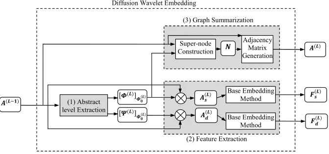
[image:11.612.138.474.134.291.2]Diffusion Wavelet Embedding
Figure 1: The flowchart of one level of DWE. Three basic sub-routines are determined in bold face, each of which is described in its corresponding paragraph.
4. Proposed method
A multi-resolution approach for graph comparison needs to extract different
abstract levels3 of graphs and be able to compare the corresponding abstract
levels with each other. The proposed multi-resolution method called diffusion
wavelet embedding (DWE) method, relies on diffusion wavelet decomposition
220
for extracting these abstract levels. Subsequently, a graph feature extraction
method is used to enable efficient comparison between the graphs extracted at
different levels. The flowchart of one level of DWE is drawn in Fig. 1.
As it can be seen, DWE consists of three sub-routines: 1) Abstract level
extraction, 2) Feature extraction, and 3) Graph summarization. In the first
225
sub-routineA(L−1), the adjacency matrix of the previous abstract level, is
pro-cessed through the diffusion wavelet and [Φ(L)]
Φ(0L) and [Ψ
(L)]
Φ(0L), the bases of
approximation and detail subspaces of Lth abstract level, are returned. Note
thatL, the abstract level, is not the same as the resolution levell. The summary
and detail features of this level,Fs(L)andFd(L), are extracted in the second
sub-230
3One abstract level is identified with multiple resolution levels in the diffusion wavelet
decomposition. As it will be described, each abstract level encapsulates the diffusion wavelet
computations for one or more resolution levels. In this article, the superscript(L)indicates
theLthabstract level, while the subscript
routine through applying a base feature extraction method onA(sL) and A(dL),
the symmetric matrices obtained from the mappings of the input graph to the
approximation and detail subspaces. Finally, the next abstract graph, A(L),
is built through graph summarization sub-routine and transmitted to the next
level for further processing. This sub-routine is performed in two steps. In the
235
first step, the set of super-nodes,N, are constructed usingA(L−1)and [Φ(L)] Φ(L)
0 and in the second step, the adjacency matrix of the abstract graph is generated
fromA(L−1) andN.
4.1. Abstract level extraction
The objective here is to extract the next abstract level from the input graph
through application of the diffusion wavelet. We begin with the input graphG
with adjacencyA0. This matrix can be written as
A= [u1, u2, . . . , u|V|], (6)
where ui is the ith column of the adjacency matrix. The jth element of ui,
240
Ai,j, represents the power of connection between the vertices vi and vj. The
strategy is to apply the diffusion wavelet decomposition on diffusion operator
T to reduce the dimension of the approximation subspace. At each application
of the wavelet decomposition the level of detail is reduced, but not necessarily
enough to allow us to represent the approximation space in a lower dimension.
245
As a result, we may need to apply the decomposition multiple times before we
can reduce the dimensionality of the subspace. Each dimensionality reduction
is anabstract level and contains one or moreresolution levels.
LetS0 be the approximation subspace in which the abstract graph of level
L−1, G(L−1), and its adjacency matrix, A(L−1), are defined. Assume that
at abstract level L, a dimension reduction occurs after m(L) diffusion wavelet
such that
S0=S1=· · ·=Sm(L)−1⊃Sm(L), (7)
whereSlis the approximation subspace obtained from applying diffusion wavelet
decompositionltimes. In the intermediate subspaces the number of dimensions
250
is equal to the number of dimensions of S0, so each vertex is described with
the same number of coordinates as the vertices inG(L−1). On the other hand,
the dimension reduction inSm(L) means that every vertex can be represented
by fewer coordinates and the number of vertices describing the graph can be
reduced.
255
4.2. Feature extraction
At the current level, [Φ(mL()L)]Φ(L)
0 and [Ψ
(L)
m(L)]
Φ(0L) are the bases of the
approx-imation and the detail subspaces, which are derived through eq. 4 and eq. 5,
respectively. We need to mapA(L−1)into these subspaces in order to find the
graph representation at levelL. The vertex coordinates are mapped into these
subspaces by projection onto the bases:
X(L)=A(L−1)×[Φ(mL()L)]
Φ(0L), (8)
Y(L)=A(L−1)×[Ψm(L()L)]Φ(L)
0 , (9)
whereX(L) represents the summary embedding andY(L)represents the detail
embedding. The resultingX(L)andY(L)matrices are not square because of the
reduction in dimensionality. For example,X(L) is a|S
0| × |Sm(L)|matrix. For yielding real-valued eigenvalues and eigenvectors (which are the raw materials
of almost all the spectral embedding methods), the processed matrix needs to
be square and symmetric. This task is done through the following equation:
There is a similar equation for the detail space. The resultingA(sL) and A(dL)
have the same dimensions as A(L−1), i.e. |S0| × |S0|, but they possess less
information. This kind of representation allows us to identify the original graph
vertices with the reduced resolution version. In fact the mappings of the input
260
graph to the approximation and detail subspaces should have the dimensions
of|Sm(L)| × |Sm(L)| and (|S0| − |Sm(L)|)×(|S0| − |Sm(L)|), respectively. But it
should be noted that the resulting matrices A(sL) and A(dL), are not used as a
lower resolution representations. These matrices are used as the inputs of some
base graph feature methodf(G) to extract the graph features in the next step.
265
The proposed diffusion wavelet embedding method for this purpose is defined
as follows:
Definition 1. Diffusion Wavelet Embedding (DWE):Given the set of abstract
subgraphs A = {A} ∪ {A(sL)|L = 1. . . ρ} ∪ {A(dL)|L = 1. . . ρ} for reference
graph G∈ G and the base embedding method f : G → Rm, diffusion wavelet
embeddingF is:
Ff,A:G →Rm×(2ρ+1)
Ff,A(G) = [f(A), f(A(1)s ), f(A(2)s ), . . . , f(A(sρ)),
f(A(1)d ), f(Ad(2)), . . . , f(A(dρ))].
(11)
4.3. Graph Summarization
To proceed with the DWE at the next abstract level, a graph summarization
method is needed. Here a diffusion wavelet-based method is proposed which
de-270
rives the abstract graph,A(L), from the input graph,A(L−1), through applying
the basis of the summary space [Φm(L)]Φ0 to it. This procedure consists of two
steps: 1) super-node construction and 2) adjacency matrix generation. In the
first step, the vertices of the input graph should be partitioned into super-nodes
which play the role of the vertices of the graph at the next level. For this
pur-275
pose, V(G(L−1)) is divided into two groups: the participant and the deleted
vertices. These two classes of vertex are defined during the wavelet
Aas the first basis. The next basis is formed through orthogonalization of the
vector with greater difference to its image on the basis constructed so far. This
280
process is repeated until the difference is lower than a pre-specified threshold.
The columns which participate in basis construction through orthogonalization
indicate participant vertices (with the indices included inJm(L)) and the vertices
which are discarded up to desired threshold are called deleted vertices.
Each participant vertex is considered as the representative of a super-node.
285
So there exist |Jm(L)| super-nodes, N = {n1, n2, . . . , n|J
m(L)|}. Now it is time
to assign the deleted vertices to the super-nodes. Two approaches are
pro-posed here for this purpose: Nearest Neighbor (NN) and Maximum
Participa-tion (MP).
In NN approach, the deleted vertices are assigned to their nearest super-node
290
in the target space. For this purpose, a 1NN classifier is used while the columns
of X(L) corresponding to the participant vertices are the training points and
the columns of X(L) corresponding to the deleted vertices are the test points.
X(L)is computed through eq. 8.
Motivated from [38], in the MP approach, thejthentry of the extended
scal-ing function correspondscal-ing to the super-nodenk, is considered to be the amount
of participation ofvj in constructing this super-node. Thus, each deleted vertex
vj is assigned to the super-node nk which has more participation in making
this super-node relative to the others. In other words,vj shows more tendency
to make nk rather than other super-nodes. This heuristic is expressed in the
following equation:
S(vj) = argmax k,k∈Jm(L)
ϕ(mL()L),k(j), (12)
whereS(vj) is the super-node which the deleted vertex vj is assigned to.
295
After assigning all the deleted vertices to the super-nodes, partitioning the
members of V(G(L−1)) into super-nodes, N = V(G(L)), is completed. The
next step is to insert edges between these vertices and formE(G(L)) through
:
:
0 1 1 0 0 0 1 0 1 0 0 0 1 1 1 1 1 1 0 0 0 1 0 1 0 0 0 1 1 0
0 1 1 0 0 1 0 1 0 0 1 1 2 1 1 0 0 1 0 1 0 0 1 1 0 0 1 1 0 0 0
1 0 1 0 0 0 1 1 0 1 0 0 0 0 1 0 1 1 0 0 0 1 0 1 0 0 0 1 1 0
1 2 3 4 5 6
1 2 3 4 5 6
1 2 {3,4}
5 6
1 2 3 4 5 6
1 2 {3,4}
5 6
[image:16.612.143.470.120.309.2]1 2 {3,4} 5 6
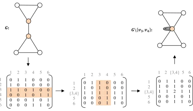
Figure 2: An example for vertex identification on the vertices of the super-nodes.
is used, and an example of this operation is shown in Fig. 2. Two vertices
300
{v3, v4} are merged in the natural way by including any edges external to the
pair. Internal edges become self-loops. The resulting graphG\{v3, v4}is shown
at the top-right of Fig. 2.
4.4. The Algorithm
The algorithm of the proposed method is shown in Algorithm 1. The inputs
305
of this algorithm are the graph adjacency matrix A, the number of abstract
levelsρ, the diffusion wavelet threshold ε, the super-node construction method
θ, and the base embedding methodf :G →Rm. The output is them×(2ρ+ 1)
dimensional feature matrix F. At first, the embedded vector of the reference
graph, f(A), is considered as the first column of the feature matrix F. The
310
main body of the algorithm is repeatedρtimes. In each iteration, the operation
corresponding to a single abstract level is performed. In step (i), each time,
one level of diffusion wavelet is applied on the transition matrix T through
the functionDiffusion Wavelet. If the dimension of the approximation
sub-space is reduced, this subsub-space is considered as the approximation subsub-space of
315
on the projection of T on the scaling functions. The inputs of the function
Diffusion Waveletare the transition matrixT, the extended scaling functions
of the previous resolution level [Φl−1]Φ0, the basis of the initial space Φ0, and
the threshold ε. Its outputs are the mapping of transition matrix T on the
320
approximation subspace of the current resolution level, the extended scaling
and wavelet functions of this level ([Φl]Φ0,[Ψl]Φ0), and the indicesJl, Klof the
dimensions involved in the summary and detail spaces of T, respectively. In
step (ii), The vertex coordinates in the previous abstract level is mapped to the
approximation and wavelet subspaces, the resulting matrices are converted to
325
the square symmetric ones, and their embedded vectors are inserted into
fea-ture matrix F. In step (iii), every participant node initiates a super-node as
its representative. The super node of every deleted node is either set to be its
nearest representative in the mapped coordinates or selected according to eq.
12, depending on the choice of methodθ being NN or MP. For the first case,
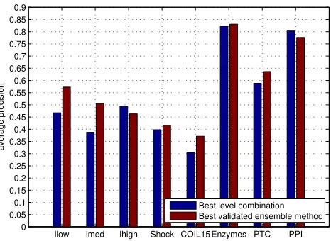
330
determining the 1-nearest neighbor is equivalent to finding the nearest point
in terms of Euclidean distance (or any other distance metric) and the mapped
coordinates is fetched from matrixX. In step (iv), the adjacency matrix of the
new abstract graph is computed through applying function vertex identify
each time on the members of one super-node. This function takes the adjacency
335
matrixAand the super-nodesN(i) as input and identifies the members ofN(i)
in the output adjacency matrix. Finally, the transition matrix and its space are
updated for the next iteration.
The time complexity of the algorithm is principally dependent on either the
base embedding method or the diffusion wavelet decomposition process. The
340
diffusion wavelet decomposition relies on QR decomposition of a matrix which is
typicallyO(|V|3), with the usual speed-up for sparse graphs. This process must
be repeated for each wavelet level, but in the experiments here, the number of
levels required is small (1 in half of the cases and less than 7 in 93 percent of
the cases). We use the Laplacian spectrum embedding method, which is again
345
O(|V|3) and the overall complexity is O(l|V|3) where l is the total number of
Algorithm 1The algorithm of diffusion wavelet embedding method.
Inputs: A: adjacency Matrix
ρ: Number of abstract levels
ε: Diffusion wavelet precision
θ: the super-node construction method (NN or MP)
f: the base embedding method
Output: F: the feature matrix
1: Addf(A) as a column of matrixF
2: T ←Transition Matrix(A)
3: S←S0
4: forL= 1, . . . ,ρdo
◃(i). Abstract level extraction
5: Φ0←an orthonormal basis whichε-spansS
6: J0← {1. . .col(T)}
7: l←1
8: whileJl−1=Jldo
9: [[Φl]Φ0,[Ψl]Φ0,(Jl, Kl), T]←Diffusion Wavelet(T,[Φl−1]Φ0,Φ0, ε)
10: l←l+ 1
11: end while
◃(ii). Feature extraction
12: X←A×[Φl]Φ0
13: As←XXT
14: Ad←(A×[Ψl]
Φ0)(A×[Ψl]Φ0)T
15: Addf(As) andf(Ad) as two columns of matrixF
◃(iii). Graph Summarization: Super-node construction
16: for every participant nodei, additoS(i)
17: for every deleted nodei, additoS
(
argmin
k,k∈Jl
∥X(Jl(k))−X(i)∥2 ifθis NN
argmax
k,k∈Jl
Φl(i, k) ifθis MP
)
◃(iv). Graph Summarization: Adjacency matrix generation
18: for everyS(i),A←vertex identify(A,members ofS(i))
19: T ←Transition Matrix(A)
20: S← ⟨{ϕl,k}k∈Jl⟩
As it can be seen, unlike the previous embedding methods which return a
feature vector for each graph, the output of DWE is a feature matrix.
5. Experiments
350
In this section, we report the results of experiments to show the effectiveness
of the summarization and the embedding method. To begin, we examine the
properties of the graph summarization; in section 5.1 we use a toy example
to illustrate how the graph reduces in resolution whilst maintaining the key
structures. In section 5.2 we evaluate the accuracy of the summarization using
355
synthetic data with varying structure.
In section 5.3 we evaluate the performance of multi-scale representation with
respect to edit distance, which is considered the gold-standard measure of graph
dissimilarity. Finally, in section 5.4 we explore whether real data has the
multi-scale properties which make our approach useful and compare the performance
360
of the method with other state-of-the-art algorithms on real datasets.
In these experiments, three abstract levels are used in addition to the base
level. So the feature vector set is{f(A), f(A(1)s ), f(A(2)s ), f(A(3)s ), f(A(1)d ), f(A(2)d )
, f(A(3)d )}. The base embedding method is Laplacian spectrum, which is simple
and powerful. The classification accuracies are estimated using 5NN classifier.
365
The reported values are the averages of 10 separate runs of 5-fold cross
valida-tion.
5.1. Toy example for summarization
In this section, the summaries of a sample graph are represented for
compar-ison between NN and MP approaches in super-nodes construction. This graph,
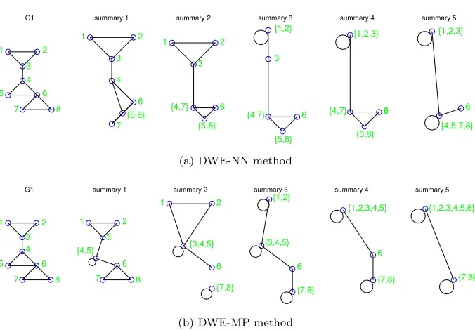
370
G, illustrated in Fig. 3a has three triangle structures composed of three node
sets {1,2,3}, {4,5,6}, and {6,7,8}. The second and the third triangles are
closer to each other and they are separated from the first triangle by means
of the edge{3,4}. It is expected for an appropriate summarization method to
encapsulate the vertices of each triangle into a separate super-node in initial
ab-375
G1 summary 1 summary 2 summary 3 summary 4 summary 5 1 2 3 4 5 6 7 8 1 2 3 4 {5,8} 6 7 1 2 3 {4,7} {5,8} 6 {1,2} 3 {4,7} {5,8} 6 {1,2,3} {4,7} {5,8} 6 6 {1,2,3} {4,5,7,8} 6
(a) DWE-NN method
G1 summary 1 summary 2 summary 3 summary 4 summary 5
1 2 3 4 5 6 7 8 1 2 3 {4,5} 6 7 8 1 2 {3,4,5} 6 {7,8} {1,2} {3,4,5} 6 {7,8} {1,2,3,4,5} 6 {7,8} {1,2,3,4,5,6} {7,8}
[image:20.612.138.476.122.357.2](b) DWE-MP method
Figure 3: The example for different super-node construction approaches in proposed graph summarization.
in further iterations. As shown in Fig. 3a, NN approach which clusters nodes
with similar relations in every step, could not differentiate between the second
and the third triangles which are located close to each other, but it could specify
the coarser node clusters in further steps. As Fig. 3b exhibits, MP approach
380
met the first expectation by constructing a node cluster for each triangle up
to the third summary level (however the super-node members are not as we
expect), but the coarser node clusters could not be established in further steps
using this approach, as the separating structure of edge {3,4} disappeared in
initial summarization steps. It can be concluded that using NN approach offers
385
more hope for constructing suitable medium and large size super-nodes, but
the impact of imprecise small super-nodes on overall summarization accuracy
5.2. Accuracy of summarization on random graphs
The previous section exhibited some behaviors of NN and MP approaches
390
in super-node construction. In order to judge between these two approaches,
they should be applied on a set of graphs with known multi-scale structures.
We prefer to use a synthetic graph set rather than a real one. The reason is
twofold. First, there is not a straightforward method to realize the inherent node
clusters in a real dataset, while in a synthetic dataset, the composition of the
395
inherent node clusters is under control. Second, although the overall accuracy of
DWE method using either of these two super-node construction approaches can
be estimated on real datasets (as in section 5.4), we cannot conclude from the
overall accuracy that the differences are merely due to the difference between
the selected super-node construction methods, because the final results affect by
400
the subsequent steps as well. The behaviors of these steps may vary in applying
on different structured graphs resulted from NN and MP approaches.
In the synthetic graph set, we composed some inherent node clusters called
communities such that they have many within-cluster relations but a few
between-cluster relations. The members of these communities are recorded for estimating
405
the accuracies of NN and MP approaches, in the following. We use a synthetic
graph set composed of 100 random graphs in this experiment. The number of
communities and the number of vertices included in each community are picked
randomly from the sets{2,3,4} and {6,7,8}, respectively. These numbers are
chosen as a compromise between providing a test for the graph summarization
410
algorithm, and the computational complexity of testing on large sets of large
graphs. Every vertex has 4 to 8 adjacent vertices within the community and
every community has 1 to 4 adjacent communities. The adjacent vertices which
connect the communities are picked randomly and every two graph
communi-ties are connected through at most 1 edge. The graphs are connected. Some of
415
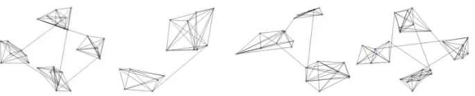
the synthesized graphs are drawn in Fig. 4. These graphs have a community
structure which varies in size and number.
To estimate the node clustering accuracy, the last level super-nodes with
Figure 4: Some of the random graphs synthesized for comparing NN and MP approaches against each other.
Table 1: The estimation of node clustering accuracy for NN and MP approach.
Method #homos #heteros #all %SN Cprecision
NN 3266 655 3921 83.2951
MP 2318 917 3235 71.6538
subsets of their vertices are checked for being in the same community. We call
the relation of being in the same community as homogeneity and that of being
in different communities as heterogeneity. The number of homogeneities and
heterogeneities in every graph is computed and the results are summed over all
graphs to obtain the values #homosand #heteros, respectively. The precision
of every super-node construction method is estimated as follows:
SN Cprecision= #homos
#all , (13)
where #all= #homos+ #heterosis the total number of two subsets checked
for all graphs. The results are tabulated in Table 1. As it can be seen from the
#all column, NN approach can cluster more nodes and obtain more abstract
420
graphs, additionally its #homosand #heteros are greater and less than their
counterparts in MP approach, respectively. Thus we use NN approach in
super-node construction from now, as its estimation of super-node clustering accuracy is
better than MP approach.
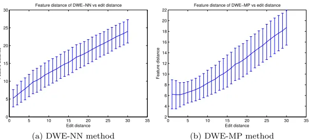
5.3. Following the edit distance
425
Graph edit distance between two graphs is defined as the minimum cost
edit operations (e.g. edge deletion) needed for transforming first graph into
of two graphs. The feature distance of an appropriate embedding method is
expected to follow the graph edit distance (which is accurate but expensive to
430
compute). In our case, if two graphs have a small edit distance from each other,
the distance of their DWE feature vector should be small as well and vice versa.
Our experiment for studying this requirement is as follows.
A seed Delaunay triangulation graph, shown in Fig. 5, is generated with 100
vertices, the (x, y) coordinates of which are the real numbers picked randomly
435
from the range [1−100]. We then delete successive random edges from the graph
to yield a sequence of graphs with increasing edit distance from the original.
In this way, we produce a set of graphs with known edit distance from 1 to
30. The long vector of DWE feature matrix of each graph in the sequence is
extracted and its Euclidean distance from the feature vector of the seed graph is
440
considered. This process is repeated 1000 times and the average feature distance
of graphs with each value of edit distance is computed. Fig. 6 shows this average
values in contrast to their corresponding edit distances. NN and MP approaches
are used as the super-node construction approach in DWE-NN and DWE-MP,
respectively. It can be seen that the feature distances follow the trend of the
445
edit distances, especially in DWE-NN method. However the deviation from the
mean value is considerable.
In these experiments, we use the Laplacian spectrum as the base embedding
method. It is well known that this embedding suffers from the problem of
cospectrality, which means that two graphs have the same spectrum and hence
450
the same embedding [14, 26]. As a result, the embedded distance is zero, but
the edit distance is non-zero. The diffusion wavelet embedding can alleviate this
problem because it explores multiple scales where the cospectrality problem may
not exist.
We examined a number of cospectral graph sets from [26]. Three sets of
455
Strongly Regular Graphs (SRGs) and two sets of Balanced Incomplete Block
Designs (BIBDs) are used. The DWE successfully distinguishes the cospectral
sets SRG(25,12,5,6), SRG(26,10,3,4) and BIBD(15,3,1) but not SRG(36,15,6,6)
Figure 5: The random Delauney triangulation seed graph.
0 5 10 15 20 25 30 35
0 5 10 15 20 25 30
Feature distance of DWE−NN vs edit distance
Edit distance
Feature distance
(a) DWE-NN method
0 5 10 15 20 25 30 35
2 4 6 8 10 12 14 16 18 20 22
Feature distance of DWE−MP vs edit distance
Edit distance
Feature distance
(b) DWE-MP method
[image:24.612.157.458.474.611.2]cospectrality but improves the performance of the base embedding method.
460
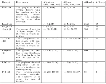
5.4. Classification accuracy of DWE on real datasets
In our final experiment, we examine the performance of DWE of real-world
data in classification problems. We use eight different graph datasets which
are common in the graph classification literature, the properties of which are
tabulated in Table 2. The first five datasets consist of object detection graphs
465
which are extracted from images; however the method of the graph extraction,
the graph sizes and their other properties are different. Among them, The
COIL15 dataset is of 15 classes of COIL-DEL dataset of [40] with the relatively
large graphs. The final three datasets are bio- and chemo-informatics datasets.
Enzymes contains graphs describing the teriary structures of protein molecules.
470
PTC is a chemical structure dataset with graphs representing atoms and bonds.
PPI is a protein-protein interaction dataset.
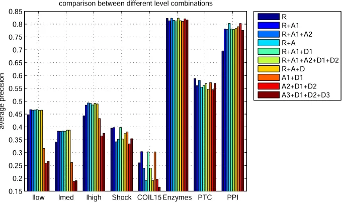
The key motivation for our method, diffusion wavelet embedding, is that
the important structures in graph datasets can occur at different scales, and
we need a scale-space representation. To explore whether this is true with real
475
data, we begin by looking at the discriminating power of the different wavelet
levels. We use three wavelet levels, and each level has an approximation and
detail feature sets. There is also a feature set for the original reference graph,
giving 7 feature sets in total. We denote these by{R, A1, A2, A3, D1, D2, D3}
where the letter refers to the type of representation, and the number to the
480
level. AandDrefer to all the approximation features and all the detail features
respectively. In the first set of experiments, we combine the chosen features
na¨ıvely, by concatenating them into a single long-vector representation. Fig. 7
shows the accuracy of some level combinations for different datasets.
It can be seen that the accuracies of different level combinations differ from
485
one dataset to another. It can be concluded that, for different datasets, the
important structural information is laid in different abstract levels. For example,
PPI consists of the relatively large graphs and the results of its two last wavelet
Table 2: The description of the tested real datasets.
Dataset Description #Vertices (min, max, ave)
#Edges (min, max, ave)
#Graphs #Classes
Llow [40] The graphs of hand-writing letters with low, medium and high distortions, respec-tively. The objective is the letter class detection.
(1, 8, 4.68) (0, 6, 3.13) 2250 15
Lmed [40] (1, 9,4.67) (0, 7, 3.21) 2250 15
Lhigh [40] (1,9,4.67) (0, 9, 4.5) 2250 15
Shock [3] The graphs of skeleton of object images. The objective is object de-tection.
(4, 33, 13.17) (6, 64, 24.33) 150 10
COIL15 [40]
The triangulation ob-ject graphs with cor-ners as vertices. The objective is object de-tection.
(18, 77, 42.73) (45, 222, 116.49) 585 15
Enzymes [2]
The graphs of pro-tein tertiary structures. The objective is to de-tect the type of en-zyme.
(2, 126, 32.63) (1, 149, 62.14) 600 2
PTC [41] The graphs of chemical compounds. The ob-jective is to detect the carcinogenicity.
(2, 109, 25.56) (2, 216, 51.92) 344 2
PPI [42] The protein-protein interaction networks. The objective is to detect the type of bacteria.
(3, 232, 109.60) (4, 3006, 864.37) 86 2
informative than its small scale interactions. This property is not observed in the
490
COIL15 dataset, even though its graphs are relatively large. The COIL15 graphs
are the object structure graphs and the reference graph consists of the subtle
structures is so important, accordingly removing this level is a big mistake.
It is clear from Fig. 7 that the chosen features have a big impact and
this varies between datasets. This supports our contention that different scales
495
are important in different datasets. Generating the long vector of the level
combinations makes the implicit assumption of the same importance for all
levels of detail and the results of Fig. 7 show that it is not an effective strategy.
Instead we need to learn which levels are important for the data. To this end,
we now use ensemble learning.
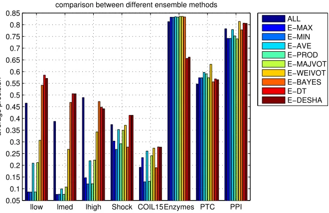
500
In ensemble learning methods, a single classifier is learned based on each
llow lmed lhigh Shock COIL15Enzymes PTC PPI 0.150.2
0.250.3 0.35 0.4 0.450.5 0.550.6 0.650.7 0.750.8 0.85
average precision
comparison between different level combinations
R R+A1 R+A1+A2 R+A R+A1+D1 R+A1+A2+D1+D2 R+A+D
[image:27.612.137.478.130.333.2]A1+D1 A2+D1+D2 A3+D1+D2+D3
Figure 7: Accuracies of applying 5NN classifier on some different level combinations’ long vectors in the tested datasets.
single classifiers [43]. Here, seven 5NN classifiers Di, i = 1, . . . ,7 are learned
for the feature vectors of the base level, each of the approximation levels and
each of the detail levels, separately. DPx(i, j) = ˆPi(Cj|x), is the probability
505
of being samplexin classj estimated by classifieri. In our case, this value is
defined as the fraction of the five nearest neighbors of samplex which are in
classj. For example, in a two class problem, if classifiericonfronted with three
neighbors of the first class and two neighbors of the second class for sample
x, we have DPx(i, .) = [0.6,0.4]. Different ensemble learning methods apply
510
different combination strategies to combine these values estimated by different
classifiers to conclude about the probability of beingxin each classj, ˆP(Cj|x).
Of course the class of the given sample x, ˆF(x), is the class with the bigger
probability value.
We explore a number of different ensemble combination methods. Max, min,
515
average, and product methods simply combine the valuesDPx(i, j), i= 1. . .7
by max, min, average, and product operators, respectively. In the majority
it. Weighted vote is similar to majority vote except that the vote of classifier
i for classj is equal to DPx(i, j). The Bayes ensemble method uses values of
520
confusion matrices of different classifiers to estimate ˆP(Cj|x). In the decision
template method, the responses of different classifiers to the training samples of
each class are structured in the decision template of that class. ˆF(x) is the class
with maximum similarity of its decision template toDPx. In Dempster-Shafer
method, the belief degree of each classifier about samplexbeing in each class
525
enter to the computations. For detailed information, please refer to [43].
Fig. 8 plots the average classification accuracies of different ensemble
meth-ods for different datasets, compared with theallstrategy which is the
classifica-tion of the long vector of all features (R+A+D in the previous section). The
results show that for different datasets, the best performing ensemble method is
530
different, but it can be selected through a validation step. For this purpose, in
each run, the accuracies of all ensemble learning methods are estimated using
4-fold cross validation and the most accurate one is selected for applying on the
test data. Fig. 9 compares the best-validated ensemble method for each dataset
against its best-performing level combination. In six out of eight cases, the
535
best-validated ensemble learning method outperforms the best-performing level
combination. Furthermore, using ensemble methods is more statistically
reason-able. Finally, the classification accuracies of DWE-NN are compared with other
embedding methods in Table 3. We chose the best-validated ensemble learning
method (best-ens) as the combination strategy for DWE-NN. The results
us-540
ing theall strategy are also inserted in order to have a fair comparison. The
other embedding methods include Laplacian spectrum (Lspec), BackTrackless
Walk [44] (BTW), Ihara Zeta Function [45] (IZF), sorted HKSs [46] (HKSsort),
histogram of HKSs [46] (HKShist), heat kernel Trace [12] (HIT), and the
coeffi-cients of heat content power series [12] (HIP). It can be observed that in half of
545
the datasets, DWE-NN using theall strategy, which simply uses the long vector
of features of all abstract levels, demonstrated better classification accuracy in
comparison with the other tested methods. However DWE-NN using the best
llow lmed lhigh Shock COIL15Enzymes PTC PPI 0.05
0.1 0.15 0.2 0.25 0.3 0.35 0.4 0.45 0.5 0.55 0.6 0.65 0.7 0.75 0.8 0.85
average precision
comparison between different ensemble methods
[image:29.612.143.473.129.343.2]ALL E−MAX E−MIN E−AVE E−PROD E−MAJVOT E−WEIVOT E−BAYES E−DT E−DESHA
Figure 8: The classification accuracies of applying different ensemble learning methods on different datasets. The base classifier is 5NN.
accuracies in comparison with the other tested embedding methods, for
classi-550
fication of the graphs in all tested datasets. The average classification accuracy
improvement for DWE in comparison with the best of the other accuracies in
the tested datasets is 6.25%.
Table 3: The classification accuracies of DWE-NN against other embedding methods for all datasets. The best classification accuracy for every dataset is indicated by * symbol. The accuracies of DWE-NN variants which are better than other tested embedding methods are demonstrated in bold face.
Llow lmed lhigh Shock coil15 Enzymes PTC PPI
Lspec 44.764 34.413 44.364 40.733 26.346 82.283 59.955 70.569 BTW 32.12 24.813 27.022 35.333 27.358 81.05 53.669 66.373
IZF 6.667 6.733 17.871 10 6.788 81.717 44.16 46.536
HKSsort 43.867 35.711 44.48 38.467 22.983 79.517 55.087 71.608
HKShist 6.782 6.667 6.72 8.8 5.798 82.167 45.375 57.105
HIT 12.382 11.742 10.68 7.4 7.605 82.583 49.818 43.673
HIP 13.076 13.356 10.769 16.267 7.604 81.083 51.324 48.333 DWE-NN
(best-ens)
57.271* 50.547* 46.276* 41.667* 37.103* 83.05* 63.629* 77.634*
DWE-NN (all)
[image:29.612.135.514.514.624.2]llow lmed lhigh Shock COIL15 Enzymes PTC PPI 0
0.05 0.1 0.15 0.2 0.25 0.3 0.35 0.4 0.45 0.5 0.55 0.6 0.65 0.7 0.75 0.8 0.85 0.9
average precision
[image:30.612.190.423.123.293.2]Best level combination Best validated ensemble method
Figure 9: The average classification accuracies of the best-performing level combination and the selected ensemble learning for all datasets.
6. Conclusion
In this article, Diffusion Wavelet Embedding (DWE) is proposed which is
555
a multi-resolution embedding method using diffusion wavelet. This method
maps the reference graph to the approximation and detail subspaces of different
abstract levels and embeds each of these mappings into vector space using a
base embedding method. The abstract graphs of different levels are constructed
by applying a diffusion wavelet based summarization method on the abstract
560
graph of the previous level.
The graph summarization using diffusion wavelet is a good option for
dis-covering the inherent node clusters within the graphs. The nearest neighbor
approach for super-node construction and the vertex identification for adjacency
matrix generation are appropriate operators for graph summarization.
565
DWE can decrease the cospectrality effects by adding the features of different
levels to the base feature set. This method removed the cospectrality effect in
three out of five tested sets. DWE uses the information of eigenvectors for
mapping the graph into the approximation and detail subspaces at one hand
and the eigenvalues to extract the information from these mappings at the other
570
sufficient for reconstructing the graph uniquely, this method has a good quality
for cospectrality reduction.
DWE can improve the classification accuracy in the wide range of
applica-tions, using the advantages of diffusion wavelet as a powerful tool for
discov-575
ering the small and large scale structures within the graph. Five image object
detection datasets with different graph extraction methods and three chemical
datasets with different graph structures are tested and DWE enhanced their
classification accuracies.
The scale of the most informative structures of the graphs differs from one
580
dataset to another. So, different level combinations have different performances
on different datasets. Utilizing the ensemble learning methods for combining the
information gathered from different levels is a suitable strategy, provided that
the more appropriate ensemble method for the special application is applied.
The experimental results suggest that the multi-resolution graph embedding
585
is a promising approach provided that the large scale descriptions of the graphs
are extracted precisely. For future work a validation phase for exploring the most
informative combination of the abstraction levels can be applied. A validation
method should be adopted to set the number of the abstraction levels and the
threshold of the diffusion wavelet. The roles of the class number, the graphs
590
[1] A. K. Debnath, R. L. Lopez de Compadre, G. Debnath, A. J. Shusterman,
C. Hansch, Structure-activity relationship of mutagenic aromatic and
het-eroaromatic nitro compounds. correlation with molecular orbital energies
and hydrophobicity, Journal of medicinal chemistry 34 (2) (1991) 786–797.
[2] L. Bai, E. R. Hancock, Depth-based complexity traces of graphs, Pattern
Recognition 47 (3) (2014) 1172–1186.
[3] L. Bai, L. Rossi, A. Torsello, E. R. Hancock, A quantum Jensen–Shannon
graph kernel for unattributed graphs, Pattern Recognition 48 (2) (2015)
344–355.
[4] A. Lubiw, Some NP-complete problems similar to graph isomorphism,
SIAM Journal on Computing 10 (1) (1981) 11–21.
[5] B. Luo, R. C. Wilson, E. R. Hancock, Spectral embedding of graphs,
Pat-tern recognition 36 (10) (2003) 2213–2230.
[6] M. M. Luqman, J.-Y. Ramel, J. Llad´os, T. Brouard, Fuzzy multilevel graph
embedding, Pattern Recognition 46 (2) (2013) 551–565.
[7] J. Gibert, E. Valveny, H. Bunke, Graph embedding in vector spaces by
node attribute statistics, Pattern Recognition 45 (9) (2012) 3072–3083.
[8] K. Riesen, H. Bunke, Classifier ensembles for vector space embedding
of graphs, in: International Workshop on Multiple Classifier Systems,
Springer, 220–230, 2007.
[9] R. R. Coifman, M. Maggioni, Diffusion wavelets, Applied and
Computa-tional Harmonic Analysis 21 (1) (2006) 53–94.
[10] D. M. Cvetkovi´c, P. Rowlinson, S. Simic, Eigenspaces of graphs, 66,
Cam-bridge University Press, 1997.
[11] P. Ren, R. C. Wilson, E. R. Hancock, Graph characterization via Ihara
[12] B. Xiao, E. R. Hancock, R. C. Wilson, Graph characteristics from the heat
kernel trace, Pattern Recognition 42 (11) (2009) 2589–2606.
[13] B. N. Parlett, D. S. Scott, The Lanczos algorithm with selective
orthogo-nalization, Mathematics of computation 33 (145) (1979) 217–238.
[14] R. C. Wilson, P. Zhu, A study of graph spectra for comparing graphs and
trees, Pattern Recognition 41 (9) (2008) 2833–2841.
[15] A. J. Schwenk, Almost all trees are cospectral, New directions in the theory
of graphs (1973) 275–307.
[16] W. H. Haemers, E. Spence, Enumeration of cospectral graphs, European
Journal of Combinatorics 25 (2) (2004) 199–211.
[17] C. D. Godsil, B. McKay, Constructing cospectral graphs, Aequationes
Mathematicae 25 (1) (1982) 257–268.
[18] R. C. Wilson, E. R. Hancock, B. Luo, Pattern vectors from algebraic graph
theory, IEEE Transactions on Pattern Analysis and Machine Intelligence
27 (7) (2005) 1112–1124.
[19] V. Bulitko, N. R. Sturtevant, J. Lu, T. Yau, Graph Abstraction in
Real-time Heuristic Search., J. Artif. Intell. Res.(JAIR) 30 (2007) 51–100.
[20] A. Rensink, E. Zambon, Pattern-based graph abstraction, in: International
Conference on Graph Transformation, Springer, 66–80, 2012.
[21] A. Torsello, E. R. Hancock, Graph embedding using tree edit-union,
Pat-tern recognition 40 (5) (2007) 1393–1405.
[22] A. Shokoufandeh, D. Macrini, S. Dickinson, K. Siddiqi, S. W. Zucker,
In-dexing hierarchical structures using graph spectra, IEEE Transactions on
Pattern Analysis and Machine Intelligence 27 (7) (2005) 1125–1140.
[23] P. Ren, R. C. Wilson, E. R. Hancock, Spectral embedding of feature
in Pattern Recognition (SPR) and Structural and Syntactic Pattern
Recog-nition (SSPR), Springer, 308–317, 2008.
[24] B. Xiao, A. Torsello, E. R. Hancock, Isotree: Tree clustering via metric
embedding, Neurocomputing 71 (10) (2008) 2029–2036.
[25] B. Xiao, E. R. Hancock, R. C. Wilson, Geometric characterization and
clustering of graphs using heat kernel embeddings, Image and Vision
Com-puting 28 (6) (2010) 1003–1021.
[26] D. Emms, S. Severini, R. C. Wilson, E. R. Hancock, Coined quantum walks
lift the cospectrality of graphs and trees, Pattern Recognition 42 (9) (2009)
1988–2002.
[27] F. Escolano, E. R. Hancock, M. A. Lozano, Birkhoff polytopes, heat kernels
and graph complexity, in: Pattern Recognition, 2008. ICPR 2008. 19th
International Conference on, IEEE, 1–5, 2008.
[28] B. Bonev, F. Escolano, D. Giorgi, S. Biasotti, Information-theoretic
selec-tion of high-dimensional spectral features for structural recogniselec-tion,
Com-puter Vision and Image Understanding 117 (3) (2013) 214–228.
[29] M. Farge, Wavelet transforms and their applications to turbulence, Annual
review of fluid mechanics 24 (1) (1992) 395–458.
[30] P. Kumar, E. Foufoula-Georgiou, Wavelet analysis for geophysical
applica-tions, Reviews of geophysics 35 (4) (1997) 385–412.
[31] T. Li, Q. Li, S. Zhu, M. Ogihara, A survey on wavelet applications in data
mining, ACM SIGKDD Explorations Newsletter 4 (2) (2002) 49–68.
[32] D. Shuman, S. K. Narang, P. Frossard, A. Ortega, P. Vandergheynst, Signal
Processing on Graphs, Signal Processing (2/35).
[33] M. Crovella, E. Kolaczyk, Graph wavelets for spatial traffic analysis, in:
Computer and Communications. IEEE Societies, vol. 3, IEEE, 1848–1857,
2003.
[34] R. Wagner, V. Delouille, R. Baraniuk, Distributed wavelet de-noising for
sensor networks, in: Proceedings of the 45th IEEE Conference on Decision
and Control, IEEE, 373–379, 2006.
[35] W. Wang, K. Ramchandran, Random multiresolution representations for
arbitrary sensor network graphs, in: 2006 IEEE International Conference
on Acoustics Speech and Signal Processing Proceedings, vol. 4, IEEE, IV–
IV, 2006.
[36] D. K. Hammond, P. Vandergheynst, R. Gribonval, Wavelets on graphs
via spectral graph theory, Applied and Computational Harmonic Analysis
30 (2) (2011) 129–150.
[37] S. K. N. Gudivada, Applications of Diffusion Wavelets .
[38] C. Wang, S. Mahadevan, Multiscale Analysis of Document Corpora Based
on Diffusion Models., in: IJCAI, 1592–1597, 2009.
[39] H. Bunke, On a relation between graph edit distance and maximum
com-mon subgraph, Pattern Recognition Letters 18 (8) (1997) 689–694.
[40] K. Riesen, H. Bunke, IAM graph database repository for graph based
pat-tern recognition and machine learning, in: Joint IAPR Inpat-ternational
Work-shops on Statistical Techniques in Pattern Recognition (SPR) and
Struc-tural and Syntactic Pattern Recognition (SSPR), Springer, 287–297, 2008.
[41] G. Li, M. Semerci, B. Yener, M. J. Zaki, Effective graph classification based
on topological and label attributes, Statistical Analysis and Data Mining
5 (4) (2012) 265–283.
[42] F. Escolano, E. R. Hancock, M. A. Lozano, Heat diffusion: Thermodynamic
[43] L. I. Kuncheva, Combining pattern classifiers: methods and algorithms,
John Wiley & Sons, 2004.
[44] F. Aziz, R. C. Wilson, E. R. Hancock, Backtrackless walks on a graph,
IEEE transactions on neural networks and learning systems 24 (6) (2013)
977–989.
[45] P. Ren, R. C. Wilson, E. R. Hancock, Pattern vectors from the Ihara zeta
function, in: Pattern Recognition, 2008. ICPR 2008. 19th International
Conference on, IEEE, 1–4, 2008.
[46] R. C. Wilson, Graph Signatures for Evaluating Network Models, in:
Pat-tern Recognition (ICPR), 2014 22nd InPat-ternational Conference on, IEEE,