5-1-2008
Semi-Automated DIRSIG scene modeling from
3D lidar and passive imagery
Stephen R. Lach
Follow this and additional works at:
http://scholarworks.rit.edu/theses
This Dissertation is brought to you for free and open access by the Thesis/Dissertation Collections at RIT Scholar Works. It has been accepted for inclusion in Theses by an authorized administrator of RIT Scholar Works. For more information, please [email protected].
Recommended Citation
Stephen R. Lach
B.S. Villanova Univerity, 1996 M.S. Villanova Univerity, 1998
A dissertation submitted in partial fulfillment of the requirements for the degree of Doctor of Philosophy in the Chester F. Carlson Center for Imaging Science
Rochester Institute of Technology
May 23, 2008
Signature of the Author
Accepted by
CERTIFICATE OF APPROVAL
Ph.D. DEGREE DISSERTATION
The Ph.D. Degree Dissertation of Stephen R. Lach has been examined and approved by the dissertation committee as satisfactory for the
dissertation required for the Ph.D. degree in Imaging Science
Dr. John Kerekes, dissertation Advisor
Dr. John Schott
Dr. David Messinger
Dr. Vincent Amuso
Date
I understand that I must submit a print copy of my thesis or dissertation to the RIT Archives, per current RIT guidelines for the completion of my degree. I hereby grant to the Rochester Institute of Technology and its agents the non-exclusive license to archive and make accessible my thesis or dissertation in whole or in part in all forms of media in perpetuity. I retain all other ownership rights to the copyright of the thesis or
dissertation. I also retain the right to use in future works (such as articles or books) all or part of this thesis or dissertation.
Print Reproduction Permission Granted:
I, Stephen R. Lach, hereby grant permission to the Rochester Institute Technology to reproduce my print thesis or dissertation in whole or in part. Any reproduction will not be for commercial use or profit.
Signature of Author:
Date
Inclusion in the RIT Digital Media Library Electronic Thesis & Dissertation (ETD) Archive:
I, Stephen R. Lach, additionally grant to the Rochester Institute of Technology Digital Media Library (RIT DML) the non-exclusive license to archive and provide electronic access to my thesis or dissertation in whole or in part in all forms of media in perpetuity.
I understand that my work, in addition to its bibliographic record and abstract, will be available to the world-wide community of scholars and researchers through the RIT DML. I retain all other ownership rights to the copyright of the thesis or dissertation. I also retain the right to use in future works (such as articles or books) all or part of this thesis or dissertation. I am aware that the Rochester Institute of Technology does not require registration of copyright for ETDs.
I hereby certify that, if appropriate, I have obtained and attached written permission statements from the owners of each third party copyrighted matter to be included in my thesis or dissertation. I certify that the version I submitted is the same as that approved by my committee.
Signature of Author:
Date
The views expressed in this dissertation are those of the author and do not reflect the official policy or position of the United States Air Force, Department of Defense, or the United States Government.
Stephen R. Lach
Submitted to the
Chester F. Carlson Center for Imaging Science in partial fulfillment of the requirements
for the Doctor of Philosophy Degree at the Rochester Institute of Technology
Abstract
The Digital Imaging and Remote Sensing Image Generation (DIRSIG) model is an established,
first-principles based scene simulation tool that produces synthetic multispectral and
hyperspec-tral images from the visible to long wave infrared (0.4 to 20 microns). Over the last few years,
significant enhancements such as spectral polarimetric and active Light Detection and Ranging
(lidar) models have also been incorporated into the software, providing an extremely powerful
tool for multi-sensor algorithm testing and sensor evaluation. However, the extensive time
re-quired to create large-scale scenes has limited DIRSIG’s ability to generate scenes ”on demand.”
To date, scene generation has been a laborious, time-intensive process, as the terrain model, CAD
objects and background maps have to be created and attributed manually.
To shorten the time required for this process, this research developed an approach to reduce
the man-in-the-loop requirements for several aspects of synthetic scene construction. Through
a fusion of 3D lidar data with passive imagery, we were able to semi-automate several of the
required tasks in the DIRSIG scene creation process. Additionally, many of the remaining tasks
realized a shortened implementation time through this application of multi-modal imagery.
Lidar data is exploited to identify ground and object features as well as to define initial tree
location and building parameter estimates. These estimates are then refined by analyzing
resolution frame array imagery using the concepts of projective geometry in lieu of the more
com-mon Euclidean approach found in most traditional photogrammetric references. Spectral imagery
is also used to assign material characteristics to the modeled geometric objects. This is achieved
through a modified atmospheric compensation applied to raw hyperspectral imagery.
These techniques have been successfully applied to imagery collected over the RIT campus
and the greater Rochester area. The data used include multiple-return point information provided
by an Optech lidar linescanning sensor, multispectral frame array imagery from the Wildfire
Air-borne Sensor Program (WASP) and WASP-lite sensors, and hyperspectral data from the Modular
Imaging Spectrometer Instrument (MISI) and the COMPact Airborne Spectral Sensor (COMPASS).
Information from these image sources was fused and processed using the semi-automated
ap-proach to provide the DIRSIG input files used to define a synthetic scene. When compared to the
standard manual process for creating these files, we achieved approximately a tenfold increase in
thank Dr. John Kerekes for serving as my research advisor and mentor. It was through his initial
vision, guidance, patience and weekly feedback that this research was able to progress from an
abstract initial concept to a refined, useable process. While he let me run with many ideas, he also
had the foresight to help me avoid many dead-ends, and in doing so helped keep my research
pointed in the right direction. I would also like to thank my other committee members, Dr. John
Schott, Dr. David Messinger, and Dr. Vincent Amuso for the many hours they spent discussing
my research with me and helping me to stay on track.
I also need to acknowledge the Imaging Science teaching staff that laid the technical
founda-tions upon which I was able to complete this research. Of particular note were Dr. Roger Easton’s
optics course, Dr. Maria Helgeura’s Fourier Analysis courses, Dr. Don Light’s photogrammetry
course, Dr. Schott’s remote sensing sequence, Dr. Kerekes’ pattern recognition course, and Dr.
Harvey Rhody’s image processing courses. It is through exceptional instructors such as these that
students develop a passion for this field.
A special thanks also goes out to the DIRS staff, in particular Scott Brown, Dr. Emmett
Ien-tilucci, Dr. Rolo Raque ˜no and Cindy Schultz. Scott, Emmett, and Rolo are Associate Scientists in
the department, and their expertise allowed me to use them as a sounding board and sanity check
on numerous occasions. Cindy continually went beyond the call of duty in providing logistical
help throughout my entire time at RIT.
I have also received a significant amount of assistance from my fellow students over the past
three-and-a-half years. Of particular note are Prudhvi Gurram and Susan Munn, who spent many
hours working through the details of modern computer vision techniques with me. Mike Foster
and Derek Walvoord were also key to this research, as they both provided many important insights
and helped me refine ideas on a wide range of topics.
And of course, I owe a special debt of gratitude to my family, both immediate and extended.
In particular, I would like to thank my Uncle Stuart; it has been wonderful having a family
mem-ber who is able to clearly see solutions for the most difficult technical and mathematical issues I
have faced in this research. I also wish to thank my parents for their continual encouragement,
which has been consistently present for longer than I can remember. And most of all, I thank my
wife Michelle for her constant support throughout the many long hours required by this project.
Without her continually going over-and-above these past few years, I would certainly never have
Abstract I
List of Figures XI
1 Introduction 1
1.1 Research Objectives . . . 4
1.2 Scope . . . 7
1.3 Achievements and Contributions to Knowledge . . . 8
1.4 Dissertation Overview and Organization . . . 9
2 Background 11 2.1 Traditional Remote Sensing and Optical Imaging . . . 12
2.2 Photogrammetry . . . 17
2.3 Laser-Based Remote Sensing Systems . . . 19
2.4 The DIRSIG Model . . . 23
2.5 Current Process for DIRSIG Scene Creation . . . 25
3 Theory 29 3.1 Photogrammetry and Computer Vision . . . 30
3.1.1 Traditional (Euclidean-based) Photogrammetry . . . 30
3.1.2 Computer Vision . . . 33
3.1.3 Photogrammetry Via Projective Geometry . . . 34
3.1.3.1 Points, Lines and Planes . . . 34
3.1.3.2 Central Projection inP3 . . . . 36
3.1.3.3 Epipolar Geometry and Multiple-Image Object Reconstruction . . . 39
3.2 Iterative Optimization: The Levenberg Marquardt Algorithm . . . 41
3.3 Robust Parameter Estimation . . . 44
4 Approach 49 4.1 Extraction of the Terrain Model . . . 50
4.1.1 DTM Extraction from Lidar Data . . . 51
4.1.1.1 DTM Extraction in the Literature . . . 54
4.1.1.2 DTM Extraction Techniques Used in This Research . . . 56
4.1.2 Subsampling the DTM . . . 60
4.2 Initial Segmentation of Trees from Buildings . . . 62
4.3 Coarse Image Registration . . . 68
4.3.1 Fundamental Concepts . . . 69
4.3.2 Orthorectification of Frame-Array Imagery . . . 72
4.3.3 Georectification of Linescanner Imagery . . . 74
4.3.4 Automating the Final Transformation . . . 81
4.4 Refined Building/Tree Segmentation . . . 87
4.5 Geometric Reconstruction of Trees . . . 87
4.6 Geometric Reconstruction of Buildings . . . 90
4.6.1 Recent Approaches to Building Reconstruction in the Literature . . . 91
4.6.2 Overview of the Novel Building Reconstruction Approach . . . 96
4.6.3 Extraction of the Building’s Outer Boundary . . . 97
4.6.3.2 Line Simplification . . . 102
4.6.3.3 Boundary Regularization . . . 107
4.6.3.4 Illustration of the Boundary Extraction Process . . . 110
4.6.4 Extracting the Internal Building Structure . . . 112
4.6.4.1 Finding the Dominant Roof Planes . . . 114
4.6.4.2 Initial Roof Reconstruction . . . 121
4.6.4.3 Dealing with Internal Vertical Transitions . . . 124
4.6.5 Refining Building Models Using High Resolution Imagery . . . 127
4.6.5.1 Registering 3D Lidar Data to 2D Frame-Array Imagery . . . 127
4.6.6 Building Edge Refinement . . . 131
4.7 Spectral Assignment . . . 133
4.7.1 Using Geometric Information to Improve the ELM . . . 135
4.7.2 Brightness-Derived Orientation Mapping . . . 137
4.7.3 Additional Considerations . . . 144
4.8 Alternate Methods: Missing Image Modalities . . . 146
4.8.1 Degraded or Missing Hyperspectral Imagery . . . 146
4.8.2 Only Lidar Data is Available . . . 148
4.8.3 Only Passive Imagery is Available (No Lidar Data) . . . 149
5 Results and Discussion 151 5.1 Illustration of the Process: RIT Scene . . . 152
5.2 RIT Scene: Analyzing the Geometric Quality of the Process . . . 163
5.2.1 DTM Analysis . . . 163
5.2.2 Tree Parameter Estimation Using the Generalized Ellipsoidal Model . . . 173
5.3 Residential Scene: Building Reconstruction . . . 177
6 Summary and Conclusions 197
7 Future Work 201
A Tutorials 207
A.1 Orthogonal Least Squares:
Fitting Lines and Planes to Data . . . 208
A.2 Rotation Matrices . . . 211
A.3 Determining Whether or Not a Ray Intersects a Triangle . . . 220
A.4 Line of Intersection of Two Planes . . . 221
B DIRSIG Input Files 223 B.1 Conversion of Models to DIRSIG Compatible Files . . . 224
B.1.1 DTM Raster or Points to DTM .obj File . . . 224
B.1.2 Spectral Curve to Emissivity File . . . 225
B.2 Example DIRSIG Input Files . . . 226
B.2.1 Example DIRSIG Configuration File (.cfg) . . . 226
B.2.2 Example DIRSIG Object Database File (.odb) . . . 230
B.2.3 Example CAD Object Files (.obj) . . . 231
B.2.4 Example DIRSIG Material File (.mat) . . . 234
2.1 Digital framing camera geometry . . . 13
2.2 Digital pushbroom imager geometry . . . 13
2.3 Digital line-scanner geometry . . . 14
2.4 Concept of a hyperspectral image cube . . . 15
2.5 MISI optical train . . . 17
2.6 Lidar data collection . . . 20
2.7 3D elevation-based lidar image . . . 21
2.8 Height, intensity, and return lidar images . . . 22
2.9 DIRSIG images . . . 24
2.10 Standard process: Block diagram . . . 25
3.1 Illustration of collinearity and coplanarity . . . 31
3.2 Geometry of central projection . . . 37
3.3 Epipolar Geometry . . . 39
3.4 Approaches to 3D point recovery . . . 41
3.5 RANSAC . . . 45
4.1 New process for scene reconstruction. . . 50
4.2 DEM, DTM, DCM . . . 52
4.3 DTM block diagram . . . 53
4.4 Methods of terrain extraction . . . 55
4.5 DEM erosion filtering . . . 56
4.6 Illustration of the Modified Minimum Filter . . . 58
4.7 Slope-based DTM extraction . . . 59
4.8 Subsampling the DTM . . . 61
4.9 Segmenting buildings from trees . . . 64
4.10 Two perspective images of a single 3D object . . . 69
4.11 Orthographic projection . . . 71
4.12 3D to 2D registration . . . 72
4.13 Coordinate frames . . . 77
4.14 MISI optical path geometry model. . . 78
4.15 Simplified geometrical model of MISI’s optical path. . . 79
4.16 Mis-registration of two ortho-images . . . 82
4.17 Constructing the CRLI . . . 85
4.18 Various shapes represented by the tree model . . . 90
4.19 Determination of a group’s exterior boundary . . . 98
4.20 Exterior boundary through Hough transform . . . 99
4.21 Different definitions regarding the shape of a point cloud . . . 101
4.22 Estimation of local curvature . . . 102
4.23 The sleeve method . . . 104
4.24 Bias in the basic sleeve algorithm . . . 106
4.25 Line-segment re-alignment . . . 109
4.26 Illustration of the boundary extraction process . . . 111
4.27 Range, normal, and plane-fitting error images . . . 113
4.29 Final Segmentations . . . 121
4.30 Reconstructing a single facet . . . 122
4.31 3D facet and initial building model . . . 123
4.32 Single segment containing both a shared edge and a vertical transition . . . 125
4.33 Two potential outcomes of an undetected DLS . . . 126
4.34 Features arising from the intersection of planes . . . 128
4.35 Improving edge locations with high-resolution imagery . . . 132
4.36 Definition of angles . . . 134
4.37 Illustration of the ELM concept and modification based on target orientation . . . . 135
4.38 BDOM cases . . . 138
4.39 Ratio: direct solar to downwelled plus upwelled radiance . . . 139
4.40 Illustration of the BDOM known/unknown case solution . . . 140
4.41 Quality metricqfor BDOM rooftop example . . . 143
4.42 ELM vs. GC-ELM results . . . 143
5.1 RIT scene. . . 152
5.2 Terrain extraction . . . 155
5.3 Initial tree/building segmentation . . . 156
5.4 Simple CAD building model . . . 158
5.5 MISI georectification . . . 159
5.6 Illustration of lidar/WASP registration. . . 160
5.7 RIT Scene: Texture and material maps . . . 161
5.8 RIT Scene: Simulated image of the scene model . . . 162
5.9 DTM Comparison with USGS DEM . . . 165
5.10 DTM error images and histograms . . . 166
5.11 Raster versus point-based terrain extraction . . . 169
5.13 DTM extraction processing times . . . 172
5.14 Tree model fitting: high data density . . . 174
5.15 Tree model fitting: low data density . . . 175
5.16 Residential buildings . . . 177
5.17 CAD models for Building A . . . 178
5.18 CAD models for Building A: Nadir and front views . . . 179
5.19 Building B range and boundary images . . . 182
5.20 Building B segmentations . . . 183
5.21 Building B: 3D model results . . . 183
5.22 Building B CAD models: semi-autonomously created and manually-produced . . . 184
5.23 CAD models for Building B: nadir and front views . . . 185
5.24 Shed Scene . . . 187
5.25 Shed scene: Rall image and DTM . . . 188
5.26 Entropy image and tree locations . . . 189
5.27 Material mapping of building facets . . . 190
5.28 Synthetic images of the shed scene models . . . 191
5.29 Shed scene images: COMPASS, SAS, MPS . . . 192
5.30 A comparison of tree center locations . . . 193
5.31 Grass Spectra: SAS and MPS . . . 194
5.32 Reflectance Spectra: SAS and MPS . . . 195
A.1 Least squares residuals . . . 208
A.2 Nose, left wing, up coordinate frame . . . 212
Charles Franklin Kettering, U. S. Engineer and Inventor
1
Introduction
In recent years, the remote sensing community has seen significant advances in the development
of non-traditional imaging techniques. With the advent of commercial imaging spectrometers,
hyperspectral image analysis has been near the forefront of this boom, and algorithms exploiting
spectral information continue to evolve. However, in many cases, testing, validation and
train-ing of these algorithms requires the use of well-calibrated datasets, the generation of which can
be expensive and time prohibitive. As such, quality hyperspectral synthetic imagery can be a
tremendous asset, as often the simulated data is able to reduce or eliminate the need for costly
real-world data collection campaigns. Additionally, realistic synthetic image generation (SIG)
en-ables engineers to evaluate the final image products given the parameters of the sensor. This may
be done to evaluate an existing sensor under a host of illumination, atmospheric and geometric
scene conditions, but it may also be done before the sensor is even built. As such, SIG is often a
critical component in the design process of new sensors.
Light Detection and Ranging (lidar) systems have undergone a similar maturation in the last
decade, and the use of laser-scanning systems to produce three-dimensional imagery is now
widespread. However, even with the proliferation of this technology, many researchers are still
lacking quality data sets with corresponding truth measurements. This is especially true for those
working in the area of multi-modal image fusion, where the lidar data is augmented by imagery
from an additional sensor. In this field, accurate registration of the imagery is critical, yet
with-out truth data the quality of this registration is often difficult to ascertain. However, with a good
multi-modal SIG model, synthetic combined datasets with associated truth values are easy to
obtain. Additionally, synthetic lidar images may be used for the characterization and design of
sensors, much as they were in the hyperspectral case. For these reasons, the ability to produce
accurate simulated imagery can be of great benefit to the lidar community as well.
The Digital Imaging and Remote Sensing Image Generation (DIRSIG) model described in
Sec-tion 2.4 is a tool capable of creating this desired synthetic imagery. Given a pre-defined scene, it
generates an accurate representation of what a modeled passive electro-optical (EO) or active lidar
sensor would detect under specified conditions by modeling the relevant physical processes in the
imaging chain. Its use has been well documented in the literature (see [Ientilucci and Brown 2003]
and [Schott et al. 1999] for example), and it is currently being used in both academia and industry.
However, while it is fairly easy to model different sensor designs, atmospheric conditions and
geometries for a given scene, the current process for actually generating a DIRSIG scene is quite
involved. As a case in point, the creation of the MegaScene documented in [Ientilucci and Brown
2003] took a team of researchers well over a year to complete.
This work aims to shorten the time required for this process by reducing the man-in-the-loop
data with passive EO imagery, many of the tasks required in the scene creation process may be at
least partially automated. Additionally, most of the remaining tasks will also realize a shortened
implementation time through the application of multi-modal imagery. It is anticipated that once
the data have been collected, a scene on the order of the Megascene effort could be constructed by
a single individual in approximately three weeks, and most of this time would be applied to the
final human inspection of the results.
In addition to reducing the time required to generate a DIRSIG scene, such automated
tech-niques also facilitate the creation of an accurate simulated environment for which ground truth is
either difficult or impossible to obtain. In many practical scenarios, direct access to the region of
interest is restricted, and the scene construction must be completed solely from remotely-sensed
data. This is especially true in rapid-response disaster relief efforts and military applications. In
these instances, the ability to properly fuse all data sources in a timely manner may be as
impor-tant as the final fidelity of the resulimpor-tant model.
The techniques described in this dissertation also have a host of applications outside the realm
of synthetic scene construction. Many of these algorithms may be effectively used to generate
dig-ital city models used for urban planning, environmental planning and monitoring, and
location-based services. Additional applications include cartography, corridor mapping, flood and risk
assessment, and forestry management (See [Behan et al. 2000] and [Ma 2004]). With the
decreas-ing costs of lidar and other three-dimensional imagdecreas-ing technologies, traditional photogrammetric
efforts are likely to be replaced in many applications by multi-modal fused imaging methods.
This work focuses primarily on the development of the algorithms needed to achieve these
objectives, as well as the application of these algorithms to data collected over the RIT campus
and the surrounding area. Additional emphasis is placed on describing how well each step in the
process was performed, evaluating the effectiveness of the process taken as a whole, and
compar-ing these results to those obtained by traditional methods. While the results in general are most
the approach describes how individual techniques should be modified when certain data sources
are degraded or unavailable.
1.1 Research Objectives
This section provides a general overview of the main objectives associated with this research
ef-fort. As noted above, the primary goal of this work was to create a spectrally-accurate scene by
fusing multiple image modalities in a nearly-autonomous manner. However, early on this goal
was broken down into a series of more easily achieved task-oriented objectives. These objectives
comprised the minimum set of accomplishments necessary to adequately complete this research.
As defined in the research proposal, these tasks were as follows:
1. Develop or adapt a means to co- and geo-register image data from multiple sensing sources,
including high-resolution framed-array imagery, multi-spectral framed-array imagery,
hy-perspectral line-scanned imagery, and line-scanned lidar point clouds. The intent of this
portion of the research was to provide an accurate method of performing the registration,
and automation of this task was not required. Additional difficulties and issues that arose in
relation to the specific sensors used in this research were also to be addressed. An example
of this was the co-registering of bands from a hyperspectral sensor whose bands exhibit a
relative spatial offset, such as the Rochester Institute of Technology’s Modular Imaging
Spec-trometer Instrument (MISI). Although this requirement is discussed briefly in this work, a
more complete development is included in [Casey et al. 2007] and [Casey 2008].
2. Using the image data, extract a bare-earth Digital Terrain Model (DTM) for the desired
area. Although in many cases, an adequate terrain model may be obtained from the U.S.
Geological Survey, one of the motivations behind this work was to recreate scenes for which
ground truth is unavailable. As such, extraction of the DTM directly from the collected
to be robust with regard to location and image resolution; that is, they should work with
data from a variety of sensors operating in both rural and urban environments.
3. Identify, isolate, characterize and synthetically construct trees. Although a significant
amount of work has been done with regard to identifying and analyzing tree canopy
struc-ture, there is very little information available on the fusion of multiple image modalities for
individual tree reconstruction in densely-forested areas. This work sought to define a means
to combine the height data inherent in a lidar point cloud with traditional optical imagery
for improved tree analysis.
For DIRSIG scene generation, the geometric modelling of trees typically has been done using
commercial software such as Tree Professional [Onyx Computing Inc. 2006]. Although such
software was used to a limited extent in this research, in most cases tree geometries were
selected from a previously-defined library based on image-derived parameters.
4. Identify, isolate, and reconstruct man-made structures (buildings).Through a fused-imagery
approach, it was anticipated that buildings would be more accurately defined than through
traditional photogrammetric techniques. As a starting point in this analysis, techniques
re-lying primarily on lidar data were considered first. Although several general methods for
building reconstruction using this point data were pursued, only a variant of the method of
intersecting planar faces is fully examined in this report.
5. Derive a material map for the scene. Several aspects of the scene creation process require
access to a detailed material map. A material map is an indexed image where the pixel
value at a each location identifies the material type present at that position. The relation
between index values in the material map and associated material types is stored in a
look-up table. Traditional hyperspectral classifiers may be used as a starting point in producing
these maps, but in practice it has been found that these algorithms provide unsatisfactory
often using other imaging sources, to improve the material classification accuracy over the
area of interest. However, in most implementations of the process, high-resolution
multi-spectral imagery was used in lieu of hypermulti-spectral imagery, as we achieved notably better
registration results with the multi-spectral frame-array data.
6. Derive a means to provide texture (reflective spectral region only) to the scene. This is
typically done using a texture image (or images) that is registered to the scene, and
select-ing spectral reflectance curves based upon brightness values in these images. Additional
work was done in an effort to augment this method with techniques to apply texture when
multiple spectral curves for a given material are not available, or when the texture mapping
image is not of an adequate resolution to accurately describe the spatial variability of a given
class. However, this additional work is still being investigated, and it is not discussed in this
dissertation.
7. Assign spectra to the objects in the scene. The two approaches for this task are to use the
sensor as a field spectrometer, or to use the image data to select spectra for distinct regions
from a library of previously collected spectra. This research relies on the former technique
in the baseline approach, but handles spectral selection from a library in the cases where
hyperspectral imagery is not available.
8. Specify the quality of the entire process. One of the more difficult tasks in many technical
efforts is to accurately describe how well the requirements were met. In the research effort
at hand, this evaluation translates into deriving scene quality metrics that describe how well
the resultant scene meets the needs for which it was created. Such metrics have proven
difficult to construct when dealing with the geometric nature alone. This difficulty is even
greater when dealing with a DIRSIG scene, not only due to the added spectral dimension,
but also to the fact that in many instances, accurate scene reproduction (relative to the real
carried out at centimeter resolutions. Although an all-encompassing scene metric was
be-yond the scope of this research, a few performance measures are presented, and the resultant
scenes are evaluated according to these criteria.
9. Apply techniques to real image data.The techniques developed through this research have
been applied to real data collected over RIT and the surrounding area, and the resulting
scenes have been compared to a traditionally-produced scene, as well as to measured ground
truth.
1.2 Scope
Although many of the algorithms and techniques developed for this thesis may either be applied
directly or with slight modifications to a wide variety of image types, this research has only been
verified using a limited set of image sources. When available, lidar data are assumed to be given
in raw point form, and are only sampled to a raster grid when noted in the text. Multiple return
data are assumed as well, as is the availability of point characteristics such as 3D position, return
intensity, return number, and time of return. Average point density is typically assumed to be
greater than one point per square meter, and in many cases densities on the order of 5-10 points
per square meter are used. Points are also assumed to have already undergone whatever initial
geometric processing was required to bring the individual scan lines into alignment. This is a
reasonable assumption, since this task is usually accomplished by lidar-imaging vendors before
data delivery.
Spectral imagery is limited to the 400-2500 nm range. Beyond this region, thermal emission
be-comes significant, a condition not dealt with in this research. When performing spectral matching
to a library of spectral reflectance curves, the spectral imagery is assumed to be accurately
cali-brated, although a discussion is included as to how to handle the cases when it is not. However,
hyperspec-tral sensor as a field spectrometer, where absolute calibration is not required if calibration panels
are present in the scene, but spectral coverage should be sufficient to encompass the wavelengths
required for the scene model.
It is also assumed that distortions of all frame-array imagery have been corrected, so that these
imagers are essentially line-preserving central-projection cameras. Although methods to correct
for such distortion are well known, these refinements were neither implemented nor used on
the actual data. Specifics related to the sensors used to collect the imagery and the parameters
describing the quality of the imagery are included as appropriate throughout the dissertation.
Most of the code related to this research was written in Matlab and is available on the CD
included in the bound copies of this document. Code written by other researchers is documented
in the code only, and no attempt is made to reference this material in the dissertation. Also, it
should be emphasized that the code created in support of this research is strictly of the
”proof-of-concept” variety. Although an attempt was certainly made to ensure the programs execute quickly
and efficiently, the code was not optimized in any real sense.
1.3 Achievements and Contributions to Knowledge
The research proposed in this document contributes to the field of synthetic scene reconstruction in
several ways. Although this field has realized significant gains in recent years, most of the research
has been devoted to defining the geometry of a given scene. To date there has been very little work
done regarding the semi-autonomous construction of spatially and spectrally-accurate scenes. In
a conceptual sense, incorporating this spectral information represents a direct contribution to the
field, as such scenes are inherently more descriptive than basic geometric models.
This may similarly be viewed as an advancement to the simulated imagery work being
per-formed at RIT. By semi-automating the scene generation process, large scale scenes will be able
to be produced quickly and accurately. Additionally, through the methods proposed here, scenes
From a more technical standpoint, this work contributes to several areas. Most significant
is the novel fusion of lidar data with more traditional imaging sources. This fusion not only
includes straightforward techniques such as draping imagery over a lidar-produced CAD model
to provide material and texture information, but also contains more integrated techniques such
as using the lidar data as a weighted constraint during a photogrammetric bundle adjustment.
Additional contributions include a novel method for registering various image types (including a
technique to ortho-rectify MISI data), a new technique for performing atmospheric compensation,
a modified method for extracting the terrain from lidar data, a refined approach to building and
tree extraction and reconstruction, and an improved method of assigning spectral characteristics
to vertical surfaces.
1.4 Dissertation Overview and Organization
The remainder of this dissertation is organized as follows. An overview of the various
technolo-gies and tools relevant to this work is given in Chapter 2. Chapter 3 builds on this background and
introduces several state-of-the-art image processing techniques that the reader may be unfamiliar
with. It is here that the technical foundation for the approach will be laid. This includes brief
introductions to iterative optimization and robust parameter extraction, as well as more detailed
descriptions of modern photogrammetry and computer vision. Chapter 4 develops the baseline
approach for this research, and describes the process flow assuming all required image types are
available. This chapter also includes a brief overview of current techniques and their limitations
for each of the required major tasks. When all data sources are not available, modifications to the
baseline approach are often required, and these changes are also detailed in Chapter 4. Chapter 5
presents the results of applying the approach to real data and also provides a description of the
quality of the approach. A summary of the research is included in Chapter 6, and ideas regarding
future work and potential extensions of this work are given in Chapter 7. The included
proposed techniques, as well as a reference for the basic input files required to define a DIRSIG
2
Background
This chapter will provide an overview of several of the technologies and research fields pertinent
to the methods used throughout this research. Although not comprehensive by any means, it
should serve as an initial foundation for understanding the rest of this dissertation. Where
addi-tional background may be warranted, outside references are given; however, it is anticipated that
most readers with a basic technical foundation will be able to proceed without too much difficulty.
Specific algorithms and recent advances in these fields as they pertain to 3D object reconstruction
will not be included here. Rather, the recent work by other authors in relation to the specific
objectives addressed by this report will be presented in the relevant sections of Chapter 4.
2.1 Traditional Remote Sensing and Optical Imaging
The field of remote sensing is primarily concerned with extracting useful information about
ob-jects without actually coming into physical contact with them. In practice, this has most frequently
referred to analysis of the radiometric content of the imaged scenes, although in a strict sense,
pho-togrammetry and photo interpretation may also be considered a part of the remote sensing field.
For years, the primary method of data collection was through the use of airborne film cameras.
In recent years however, advances in digital imaging technologies have resulted in the rapid
ad-vancement of digital electro-optical (EO) imagers. Rather than recording the image data on
silver-halide crystals, digital imagers use an array of solid state sensors such as charge-coupled devices
(CCDs) and complementary metal-oxide semiconductor (CMOS) detectors to record the intensity
of the incident electro-magnetic radiation. As such, greyscale digital images are represented by a
2D array of picture elements (pixels), with each pixel having a quantized brightness value
(grey-level) associated with it. Color and other multi-band digital images may simply be thought of
as stacked layers of 2D arrays, where each layer represents the brightness values within a certain
spectral band.
EO systems are usually classified according to the general architecture of their image
forma-tion. Due to its similarity with traditional film systems, in many ways the digital framing array is
the simplest to envision. This device consists of a 2D array of detectors mounted in the focal plane
of a camera. To acquire the image, all of the detectors are exposed simultaneously, thereby
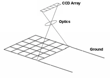
pro-ducing the same type of perspective image that is generated by a film camera. Figure 2.1 shows a
schematic illustrating the basic geometry of this design.
Another common architecture for digital imagers is the pushbroom design, which makes use
of a linear array of detectors that collects the image as the camera sweeps over the terrain. Since
the 2D image is collected as the platform moves forward, the image is acquired in temporal
in-crements. As such, the perspective of these images is similar to the standard perspective image
Figure 2.1: Digital framing camera geometry.
constant, and there will be no relief displacement in this dimension. This geometry is termedline
perspective, and the schematic for such an imager is given in Figure 2.2.
A third method for obtaining digital images is with the airborne line scanner. This system
records one pixel at a time, and uses a rotating mirror to scan lines on the ground. The sensor
plat-form advances during the collection of each line, and if the timing is correct, sequential rotations
will sweep out adjacent lines on the ground. A schematic of this imaging system is given
be-low in Figure 2.3. Although these systems are comparatively simple in design, they often exhibit
[image:32.595.218.409.542.678.2]Figure 2.3: Digital line-scanner geometry.
significant geometric distortions which must be corrected before use in many applications.
While many imaging sensors integrate the received radiance across a single spectral band to
produce a greyscale image, it is possible to modify the above designs to record multiple spectral
bands. This is commonly done to produce standard red, green, blue (RGB) color imagery, but
the number of recorded bands need not be limited to three. In general, when several (usually
defined as three to approximately ten) bands of data are collected, the system is said to be
multi-spectral. Multi-spectral images often offer tremendous advantages over conventional greyscale
images when trying to extract scene information. In many cases, objects may be identified or
classified merely by processing the relative received radiance in various spectral bands.
Over the past few years, RIT has developed a sophisticated multi-spectral imager in support
of the Wildfire Airborne Sensor Program (WASP) [McKeown 2003]. The WASP sensor combines
a high-resolution visible RGB-sensing camera with three additional IR cameras operating in the
short-wave, mid-wave, and long-wave (SWIR, MWIR, and LWIR, respectively) portions of the
IR spectrum. The color camera is an off-the-shelf Pixel Physics mapping design, and it uses a
4000×4000 pixel frame array to record its images. The three IR sensors are from the Indigo
Phoenix line, and each uses a 640×512 pixel array. These radiometric sensors are combined with
an Applanix inertial measurement unit and an on-board computer processor. When flying at an
Figure 2.4: Concept of a hyperspectral image cube [NASA JPL 2006].
IR sensors cover approximately 3 meters.
As the number of discrete spectral bands increases, we transition from multi-spectral to
hyper-spectral imaging. Hyperhyper-spectral sensors, or imaging spectrometers, record the image data at tens
to hundreds of narrow, adjacent spectral bands which essentially yields a continuous radiance
spectrum at each sample location. By so doing, a wealth of additional information is provided, as
subtle spectral features combined with the general spectral shape may be exploited in tasks such as
image segmentation and classification, target detection, and material identification. Additionally,
in many cases, these analyses may occur at sub-pixel resolutions. In order to describe the image
content of a hyperspectral dataset, the term image cube is often used. With this terminology, each
spectral band comprises an individual layer of the cube, and if we examine the grey-level values
for each layer of a given spatial (pixel) location, the spectral curve for that location is obtained.
Figure 2.4 [NASA JPL 2006] displays this concept in relation to the AVIRIS sensor.
The design approaches for multi-spectral and hyperspectral imagers are basically extensions
bands may be recorded by either placing spectral filters in front of individual pixels, or by using
a tunable filter and collecting each band’s image sequentially. The pushbroom sensor may be
modified by introducing a prism or grating device to spatially separate the spectral components
of each line, and recording the subsequent spectral-spatial line data on a 2D sensor array. In a
similar manner, a linear array may be used with a line-scanning architecture to capture multiple
band data.
Of particular interest to this research effort is the array-based COMPact Airborne Spectral
Sen-sor (COMPASS), a hyperspectral imager that captures incident radiation from 400nm to 2350nm
on a single focal plane [Simi et al. 2004], [Zadnik et al. 2004]. This sensor was developed at the
Army Night Vision and Electronic Sensors Directorate (NVESD), and was used in this research
to provide moderately-well calibrated data for the description of target reflectance spectra. The
average bandwidth of this sensor is approximately 8nm over the instrument’s spectral range, and
the spatial resolution was on the order of 1m.
This research also makes use of data from a student-designed hyperspectral line scanner. The
Modular Imaging Spectrometer Instrument (MISI) is an airborne line scanning system with
mod-ular focal planes that has been under development at RIT for the past 11 years. Originally fitted
with a VNIR spectrometer and a LWIR focal plane, it has recently been upgraded to contain a
set of SWIR, MWIR and LWIR sensors to support a fire phenomenology program [Raqueno et al.
2005]. The VNIR spectrometer uses a 6-inch rotating mirror in combination with an f/3.3
Casseg-ranian telescope, and its focal plane is sampled by two optical fiber cables. The fibers lead to two
separate 36-channel spectrometers which cover the electro-magnetic spectrum from 0.440µm to
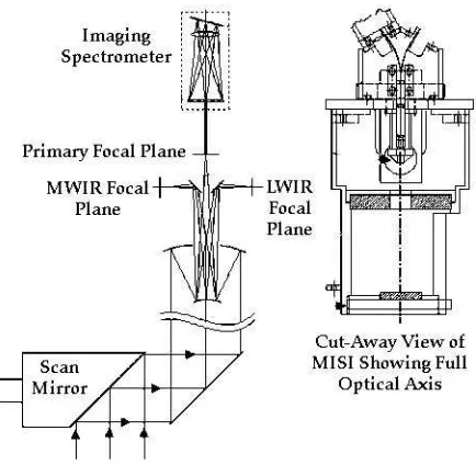
1.020µm in 0.010µm spectral bands. Some of the incident radiation is redirected from the primary
focal plane to feed five HgCdTe detectors for LWIR imaging, while secondary focal planes are
used for imaging in the SWIR and MWIR. A simple schematic of the MISI design is presented in
Figure 2.5 [DIRS Laboratory 2006].
Figure 2.5: MISI optical train.
between the two VNIR fibers in MISI causes an inherent spatial shift between the two sets of
spectral bands. This configuration causes a relatively complicated misregistration which cannot
be corrected with a simple shift, rotation or translation of the data. Coupled with aircraft roll,
pitch, and yaw variations, and elevation changes in the ground surface, these effects make
geo-rectification of the imagery quite challenging. The resolution of this issue as related to a set of
bands from a single fiber is discussed later in Section 4.3. The mismatch between spectral bands
carried on different fibers is discussed in [Casey et al. 2007] and [Casey 2008]. These sources
highlight that fact that this phenomenon severely degrades the spectral purity of each pixel for
the MISI sensor, an issue that can particularly reduce performance in sub-pixel target detection
applications.
2.2 Photogrammetry
While analysis of the radiometric content of a scene falls under the scope of remote sensing, when
the domain of photogrammetry. Although in general this field is defined as ”the art, science and
technology of obtaining reliable information about physical objects and the environment through
processes of recording radiant electromagnetic energy” [Wolf and Dewitt 2000], for the purposes
of this report, we will limit it to the metric sense, which is primarily concerned with determination
of the size, shape, orientation and location of objects in 3-dimensional (3D) space.
In order to use one or more images to extract the three-dimensional structure of objects, we
need to select a mathematical model that approximates the geometry of the imaging process. Such
a model will enable us to infer the nature of images given camera orientation parameters and the
geometry of a scene, as well as to do the 3D scene reconstruction given the images. In order to
ensure generality, we will assume that all images may be taken at oblique angles, and that the
camera system may have various distortions. However, when these distortions are accounted for,
a simple pinhole camera projection model may be assumed. We will also differentiate between
the camera coordinate system whose origin is at the projection center (typically the center of the
lens), the continuous image coordinate system (termed CIC coordinates here), whose origin is at
the center of the image, the pixel-based image coordinate system (relative to a pixel location(0, 0)
for digital images, termed PIC here), and the world (object) coordinate system. Unless otherwise
specified, all coordinate frames will be right-handed Euclidean systems.
It is common practice to separate the geometry related to the position and orientation of the
camera in space from the internal characteristics of the camera itself. Specification of the former
re-quires six parameters (three coordinates of the projection center plus three orientation angles) and
is termed exterior orientation (EOP1). The interior orientation (IOP) refers to the intrinsic camera
parameters which are needed to specify the direction of the projection ray to an object point, given
an image point and the exterior orientation [McGlone 2004]. In simple pinhole (projective center)
cameras, this may be limited to a description of the focal length; however, in most cases it also
contains parameters for principal point (the point in the image normal to the projection center)
offset and optical distortion. Interior orientation has traditionally been determined by calibration,
although recent techniques have been developed to derive at least some of these parameters from
image content. This contrasts with exterior orientation, which is usually determined from the
im-agery and in-scene control points, although recent advances in aircraft navigation technology also
often permit direct measurement of the parameters.
One the EOP and IOP have been recovered, image points representing a common location
(termed homologous or corresponding points) may be back-projected through the optical centers
of the corresponding cameras (as defined by the EOPs) and intersected in three dimensional space.
The location of this intersection point in world coordinates is the location of the object point
corre-sponding to the chosen image point. When these back-projected rays do not intersect due to errors
in the process, the point minimizing the orthogonal distance to each ray is often used to define the
object point.
The theory underlying these problems is presented in Section 3.1 and covers approaches using
both Euclidean and projective geometry.
2.3 Laser-Based Remote Sensing Systems
Lidar (Light Detection and RangingorLaser Imaging Detection and Ranging) is an active remote
sens-ing technology that measures the backscattered radiation of a transmitted laser signal to determine
properties or position of a distant object. With the continuing advances in laser design, these
sys-tems have realized a tremendous development in recent years, and many sectors of the remote
sensing field have found uses for this technology. As such, lidar is currently being used in a wide
variety of applications, including water depth measurement (bathymetry), ocean research, and
to-pographic mapping of the earth’s surface. Lidar also plays a large role in atmospheric studies, as
systems that transmit multiple wavelengths are able to determine atmospheric absorption
Figure 2.6: A simple cartoon illustrating the basic concepts of lidar data collection (aircraft and building clip art taken from [SIMoN 2006]).
systems to perform such tasks as vehicle tracking, and biological and chemical agent detection,
and automatic target recognition.
Topographic lidar systems typically are based on a laser ranging unit coupled with an
opto-mechanical line scanner, although other configurations (such as pushbroom or framing array
de-signs) have also been implemented successfully. When used in conjunction with a tightly-coupled
GPS/Inertial navigation system, these sensors are able to obtain measurements of the 3D
coordi-nates of a very large number of tightly spaced points in a short amount of time. For line-scanning
pulsed-laser systems, as the aircraft flies forward, the scanning mirror continually shifts the
view-ing angle of the laser ranger. At discrete time intervals, laser pulses are transmitted, reflected off
Figure 2.7: Perspective view of 3D lidar data using elevation-based coloring.
conjunction with the pointing angles of transmission, the precise location of the reflecting object
may be determined relative to the sensor orientation. When the sensor’s location and pointing
angles are known in absolute world coordinates, the location of the point of reflection may be
expressed in that domain as well. Figure 2.6 shows a cartoon of a generic line-scanning lidar
sys-tem in operation, and Figure 2.7 shows a resultant 3D mapping for a portion of the RIT campus.
The coloring of this image is based on an indexed scheme, where elevations (heights above the
coordinate system’s(x,y)plane) are depicted as variations in color.
For many topographic lidar sensors, point locations are not the only information extracted by
the system. In addition to the range information provided by the delay of the received signal, in
many cases the intensity of the received signal is recorded as well. This data yields information
re-lated to the reflectance properties (in the spectral region used by the source) of the illuminated
ob-ject, and may be used in post-processing to aid in point classification and feature extraction. Many
lidar sensors are also able to discriminate multiple returns from each transmitted pulse, based on
(a) (b)
(c) (d)
Figure 2.8: Lidar images: (a) Height-based image, perspective view, (b) Height-based image, nadir view, (c) Intensity-based image, (d) Return number-based image.
top of a tree and on the ground plane, and has been used successfully to identify forested regions
without relying on hyperspectral imagery or spatial image analysis (see Section 4.2, for example).
Figure 2.8 depicts the elevation map in both perspective and nadir orientations, as well as the
corresponding intensity and multiple return images for the regions surrounding RIT’s Carlson
Center for Imaging Science.
For the purposes of this dissertation, much of the theory underlying the operation of the lidar
scanner will be ignored, and the system will be treated as a ’black box’ capable of producing range
and intensity information as noted above. For additional information regarding the operation of
these systems, the reader is referred to [Argall and Sica 2003].
It should be noted that in some fields, the term ladar (Laser Detection and Ranging) is preferred
when discussing this type of laser ranging technology. A distinction between these acronyms was
which locate the position of objects, while lidar is used to describe sensors that derive
proper-ties of an object. However, in the field of 3D object reconstruction, the term lidar is used almost
exclusively. As such, lidar will be the acronym of choice for the remainder of this dissertation.
2.4 The DIRSIG Model
The DIRSIG model is a complex synthetic image generation utility that was developed at the
Digital Imaging and Remote Sensing (DIRS) Laboratory at the Rochester Institute of Technology
(RIT) over the last 20 years. The tool was originally designed to model the thermal infrared
re-gion of the electromagnetic spectrum, but was expanded several years ago to cover the full
vis-ible to long-wave infrared (0.4 to 20 micron) range. It effectively models broadband,
multispec-tral and hyperspecmultispec-tral imagery using a suite of first-principles based radiation propagation
mod-ules. These modules perform specific tasks such as predicting bi-directional reflectance functions
(BRDF), computing time and material dependent surface temperature values, and computing the
dynamic viewing geometries of scanning instruments on a moving platform. In addition to these
DIRSIG-specific modules, the tool leverages several utilities (such as MODTRAN and FASCODE)
that have been used extensively by the remote sensing community.
In 2002, a first-principles-based lidar model was incorporated into the passive radiometry
framework enabling the model to calculate arbitrary, time-gated photon counts at the sensor for
atmospheric, topographic, and volumetric backscattered returns. The DIRSIG lidar model was
first developed in [Burton 2002], and it was recently expanded by [Blevins 2005] to handle a wide
variety of complicated scene geometries, diverse surface and participating media optical
char-acteristics, and a variety of sensor models. The lidar module now includes the effect of multiple
scattering, multiple bounces from topographical targets, and absorption within non-homogeneous
finite volumes. Additionally, several noise sources are extensively modeled, such as speckle from
rough surfaces and atmospheric turbulence phase effects. As such, DIRSIG is now able to help
con-stituents (e.g. water vapor, dust, sediment, soot, etc.) may have on a Differential Absorption lidar
(DIAL) system’s ability to detect and quantify constituents of interest within volumes including
water and atmospheric plumes [Blevins 2005].
Although the passive and active models used by DIRSIG are valuable in their own right, in
many applications the ability to integrate passive EO and lidar simulations using a common scene
(and potentially common viewing geometries) is of even greater utility. The multi-modal
capabil-ities of the DIRSIG model allow designers to evaluate both passive and active approaches to
solv-ing specific imagsolv-ing problems, as well as potential fusion techniques ussolv-ing both image modalities.
Additionally, the upper performance limit for a given approach may be more easily determined
when using a common baseline scene.
Two representative synthetic images produced by the DIRSIG model are included in Figure 2.9
(Courtesy of [Blevins 2005]). The first depicts a near-infrared (passive EO) image of MicroScene1
(a small test range on the RIT campus), and the second is a topographic lidar product of a portion
of the same area.
(a) (b)
Figure 2.10: Standard process: Block diagram.
2.5 Current Process for DIRSIG Scene Creation
The current method of creating a scene for use in DIRSIG simulations is straightforward, but
unfortunately it is also quite labor and time intensive. Figure 2.10 illustrates the process via a
simple block diagram. The detailed steps in this figure (and as described below) have been taken
from [Brown 2005], [Brown 2006] and [Ientilucci et al. 2003], and represent the techniques used at
the Rochester Institute of Technology. Although the specific methods employed in creating scenes
may be somewhat different at other organizations, the fundamental principles and basic steps
remain the same.
The first step in the generation of a new scene has typically been to acquire a digital terrain
model (DTM) of the area to be modeled. For scenes based on real-world locations in the United
with success, but other sources of these data are also available. For fictional scenes, the terrain
model may be designed as desired. Once the terrain geometry has been determined, it is usually
up-sampled and registered with any relevant aerial imagery, which facilitates several of the other
steps required in the scene specification. Additionally, the terrain model needs to be facetized,
which is often done using a triangular irregular network (TIN) generation program for terrains
with a near-constant slope. It should be noted that in many cases, the terrain must be smoothed
via some form of spatial averaging before the facetized version may be created.
Once the geometric properties of the terrain have been determined, the 3D objects that will
appear in the scene must be created. These objects include buildings, trees, vehicles, and any
other structures that are not a part of the terrain model. This is often a very time-intensive process,
especially if many unique object types are desired. The geometric description of these objects can
be generated using a variety of computer aided design (CAD) tools, as long as the specific utility
is able to output the final facetized structure as a Alias/Wavefront .obj file. At RIT, most of the
geometric models have been manually drawn with the Rhinoceros [Robert McNeel and Associates
2005] CAD package, which has proven to be well suited to the task. The one exception is the
modeling of tree structures, for which we have chosen to use Tree Professional [Onyx Computing
Inc. 2006]. This software allows the user to render a host of trees, palms, and other plants of
various species and sizes and output the result as a facetized model.
Next, the spectral reflectance and emissivity data must be acquired. This is typically
accom-plished either through a direct collection (using an instrument such as a field spectrometer) or by
accessing a spectral data library. This data is then included in a materials file that will be used
when accessing the scene.
The geometric objects are then attributed with material characteristics using DIRSIG’s
Bull-dozer tool. This utility allows the user to import the Alias/Wavefront .obj files created earlier and
assign material properties to each facet. This task is also quite time consuming, as each portion of
Road, material, texture, and other background maps (scene layers) are created next [Brown
and Schott 2000]. Road maps have traditionally been created in Adobe Photoshop, due to
arti-facts left behind when segmenting real imagery. These maps are created by opening the scene
file, and adding a new layer to the image. The roads are then drawn on the new layer with the
paintbrush tool, using the scene image as a guide. The scene layer is then removed, and a black
background is added to the road map layer. Materials may be attributed either via a material map
or through a direct assignment to individual facets. Material maps usually take the form of
tradi-tional classification maps, and are often generated through traditradi-tional segmentation algorithms on
real remotely sensed imagery. Direct facet assignment of materials is achieved manually through
a modification of an object’s CAD description.
Texture maps may also be created to drive in-material spatial-spectral variations. Such
vari-ations are important in mimicking the real-world phenomenology; without them all pixels of a
given material in the scene would have the same spectral characteristics, thereby appearing more
uniform than desired. Texture maps are usually just aerial images of the scene to be modeled. In
some cases where an image of the scene was not available, a simple noise image was used instead.
Use of the texture images is quite simple. If the grass material type has 300 different spectra in
its library, the particular spectral curve for each location in the final scene is selected based on a
look-up table relating pixel values of the texture image to spectral signatures. This look-up table
is created using the statistics of both the texture image and the spectral library.
Finally, the Bulldozer utility is used to place the attributed objects onto the facetized terrain
model. If aerial imagery is available, a ”tracing paper” layer may be employed to help with object
orientation. Once the objects are placed in the scene as desired, a DIRSIG configuration file is
created to link together all of the previous files. At this point, the scene has been constructed.
Once the scene has been defined, it is a simple matter to create physically-accurate synthetic
images. First, for a standard EO imager, a sensor is defined in terms of its spatial and spectral
param-eters are defined if a lidar imager is to be used instead. Scene variables such as local time (which
dictates the relative solar positioning) and atmospheric conditions are also specified. DIRSIG is
then run to invoke the spectral ray-tracing (or photon-mapping, in the case of lidar sensors), and
the resultant synthetic imagery is produced. Various truth maps (related to such things as
mate-rial type) may also be produced, which are frequently used as the baseline when algorithms are
applied to the synthetic imagery.
Details regarding the required DIRSIG files and their proper formats are discussed later in
Appendix B. In that section, an overview of the DIRSIG file structure is presented, and several
example files are included. Additional information regarding the use of DIRSIG and proper
for-matting of the required input files may be found in [Brown 2005].
As has been demonstrated in this chapter, the current process for creating spectrally-accurate
scenes is effective but laborious and time-intensive. With the recent availability of improved lidar,
spectral and high-resolution optical sensors, we aim to reduce the effort involved in generating
such scenes through a fusion of these image modalities. Such an approach will enable automation
of many of the tasks required and will also permit increased accuracy in many instances. The
3
Theory
This chapter will provide an overview of several of the technologies and research fields pertinent
to the methods used throughout this research. Although not comprehensive by any means, it
should serve as an initial foundation for understanding the rest of this dissertation. Where
addi-tional background may be warranted, outside references are given; however, it is anticipated that
most readers with a basic technical foundation will be able to proceed without too much difficulty.
Specific algorithms and recent advances in these fields as they pertain to 3D object reconstruction
will not be included here. Rather, the recent work by other authors in relation to the specific
objectives addressed by this report will be presented in the relevant sections of Chapter 4.
3.1 Photogrammetry and Computer Vision
In recent years, researchers in the field of computer vision have been attempting to solve many
of the problems that have traditionally fallen under the auspices of photogrammetry. Computer
vision (CV) is a discipline concerned with discerning properties of the 3D world from one or more
2D digital images. However, unlike photogrammetry, whose interest is primarily in achieving
precise measurements in absolute coordinates, CV seeks a less tangibleunderstandingof the scene,
which may or may not require high accuracy or even a solution in an absolute sense. This
differ-ence in requirements arises from differdiffer-ences in application areas; while the primary products of
photogrammetric analysis are related to topographic maps, CV tends to apply its methodologies
to object recognition, autonomous vehicle navigation, and object modeling [Hartley and Mundy
1993]. Still, it takes little exposure to both fields to see that the similarities outweigh the differences,
and that both fields rely heavily on the theory of using a pinhole-type camera to understand a 3D
world from 2D projections. As such, both address methods to determine camera calibration and
pose, as well as 3D model understanding (and often model construction in absolute world
coordi-nates). In this section, we will present a few of the key concepts from traditional photogrammetry.
However, since these techniques are a part of the curriculum for many remote sensing programs,
the review will be somewhat brief. More detail will be spent on the newer CV approaches that
make use of projective geometry and homogeneous coordinates, as many researchers will be
un-familiar with these techniques.
3.1.1 Traditional (Euclidean-based) Photogrammetry
As noted in Chapter 2, if the interior orientation of the sensing system is known, we may use an
ideal (distortionless) pinhole camera model to fully describe the constrained camera geometry. In
this case, all rays coming from the object space intersect at the projection center and proceed to
the image plane without any change in direction. As such, it is easy to see that this requires any
Figure 3.1: Illustration of the geometrical principles of collinearity and coplanarity.
line. This requirement is termed thecollinearity condition, and is readily seen in Figure 3.1. In the
left image (image 1), object pointA, its imagea1, and the camera locationL1are all co-linear. The
mathematical description of this constraint may be written as
x = x0− frr11(X−XL) +r12(Y−YL) +r13(Z−ZL) 31(X−XL) +r32(Y−YL) +r33(Z−ZL)
y = y0−frr21(X−XL) +r22(Y−YL) +r23(Z−ZL) 31(X−XL) +r32(Y−YL) +r33(Z−ZL)
, (3.1)
wherexandyare the photo coordinates of the image point, f is the camera’s focal length, ther’s
describe the angular orientation of the camera (see Section A.2), (X,Y,Z)are the object
coordi-nates, and(XL,YL,ZL)are the object space coordinates of the exposure station. The termsx0 and
y0represent the location of the image principal point in image space coordinates. It is no surprise
that Equation 3.1 bears a strong resemblance to the equation representing a projective transform,
since imaging via central projection is inherently a projective process.
An extension of these concepts will also demonstrate that for two images, object pointA, its
images (a1anda2), and the exposure stations (L1andL2) all lie in a common plane. An illustration
![Figure 2.4: Concept of a hyperspectral image cube [NASA JPL 2006].](https://thumb-us.123doks.com/thumbv2/123dok_us/116286.11240/34.595.153.480.135.367/figure-concept-of-hyperspectral-image-cube-nasa-jpl.webp)