A thesis submitted for the degree of
DOCTOR OF PHILOSOPHY
by
BRIAN J. JARVIS
November 1981
Mount Stromlo and Siding Spring Observatories Research School of Physical Sciences
OiTd.
It is a pleasure to thank my supervisor Dr Ken Freeman for giving so freely his time, encouragement and support throughout the course of this work. His helpful advice did much to make possible the fulfilment of this thesis.
I would also like to acknowledge useful discussions with Dr A J Kalnajs and Professor G. de Vaucouleurs. Dr E B Newell gave valuable instruction in the operation of the PDS microden sitometer.
I am most grateful to Dr G. Illingworth for making available data before publication.
I also thank the UK Schmidt Telescope Unit at Siding Spring Observatory for the taking of plates for me with the 1.2m Schmidt telescope. Thanks also go to the Anglo-Australian Observatory for the excellent facilities provided by the Anglo-Australian
Telescope.
The use of the facilities of Mount Stromlo and Siding Spring Observatories and the assistance of the maintenance staff is also gratefully acknowledged. I am also indebted for the services
provided by the Computer Services Centre of the Australian National University. Special thanks also to Mr Keith Smith for carefully photographing and reducing the plots and photographs.
made of the structure and dynamics of the bulges of disc galaxies. Self-consistent, axisymmetric rotating models with two integrals of motion, energy and angular momentum, have been constructed for the bulges of the edge-on disc galaxies NGC 7814, 4594 and 7123. Accurate surface photometry and kinematical observations have been
combined to show that the bulges of these disc galaxies are consistent with oblate, rotationally flattened models (unlike the brighter
elliptical galaxies). The determination of V /a values for NGC 4762, m
4179 and Ham I, also confirm this finding. Under the assumption of constant M/L, the models accurately reproduce the observed two-dimensional surface brightness distributions and the observed kinematics, to the limits of the data. M/L values are derived for the three galaxies for which models were constructed, and are found to be consistent with recently observed M/L values for elliptical galaxies (M/L^ = 7 to 10) .
There are two extremes of bulge morphology in the sample. At one extreme are the peanut- and box-shaped bulges, which rotate
The thick disc components of disc galaxies, first identified by Burstein, have been modelled as the response of the bulge component to the flat potential of the disc. For the SO Galaxy NGC 4762, the models give an excellent representation of the detailed photometric
CHAPTER I INTRODUCTION AND THESIS OUTLINE 1
1.1 Introduction 1
1.2 Discussion of Previous Work 1
1.3 Thesis Outline 7
CHAPTER II DYNAMICAL MODELS OF GALACTIC BULGES 10
2.1 Introduction 10
2.2 The Models 10
(i) The Bulge 12
(ii) The Disc 15
2.3 Numerical Techniques 18
2.4 Numerical Checks 21
2.5 Projection 23
2.6 Some Model Properties 26
2.7 Summary 30
CHAPTER III OBSERVATIONAL TECHNIQUES AND DATA REDUCTION 31
3.1 Introduction 31
3.2 Photoelectric Photometry 31
(i) Acquisition 31
(ii) Reduction 33
3.3 Photographic Photometry 34
(i) Acquisition 34
(ii) Reduction 35
(a) Microphotometry 35
(h) Spot Calibration 37
(ii) Flatfielding and Wavelength Calibration 48
3.6 Velocity Determination 50
3.7 Velocity Dispersion 52
(i) Measurement Procedure 52
3.8 Comparison with NGC 3379 65
3.9 Other External Checks 72
CHAPTER IV COMPARISON: MODELS WITH OBSERVATIONS 79
4.1 Introduction 79
4.2 Selection of Galaxies 80
4.3 Fitting the Models 82
4.4 NGC 7814 83
Ci) Photometry 83
(ii) Kinematic Data 93
(Hi) Model Discussion 93
4.5 NGC 4594 99
(i) Photometry ■ 99
(ii) Kinematic Data and Model Discussion 108
4.6 NGC 7123 112
(i) Photometry 112
(ii) Kinematic Data 121
(Hi) Model Discussion 111
4.7 The V (o)/o 'v e Plane and Other Sample Galaxies 128
m o max
(i) The V (o)/o 'V/ e Plane 128
m o max
(ii) NGC 4762 131
(Hi) NGC 4179 139
CHAPTER V THE CYLINDRICAL ROTATORS 164
5.1 Introduction 164
5.2 NGC 128 164
5.3 Other Cylindrical Rotators 182
5.4 The Energy-Angular Momentum (E,J) Plane 183
5.5 Implications for Bulge Formation 187
5.6 Conclusions 194
CHAPTER VI THE THICK DISC 196
6.1 Introduction 196
6.2 The Thick Disc Model 201
6.3 Comparison with NGC 4762 205
6.4 Conclusions 211
2.1
2 . 2
3.1 3.2 3.3 3.4 3.3 3.6 3.7 3.8 3.9 3.10 3.11 4.1 4.2 4.3 4.4 4.5 4.6 4.7 4.8 4.9 4.10 4.11 4.12 4.13 4.14 4.15 4.16 4.17 4.18 4.19
Distribution of Error in Hydrodynamical Equations Model Behaviour in (K,y) and (W° y) Space
b Photographic Plate Reduction Areas
E-W Luminosity Profile of NGC 3379 and Residuals Grid of Velocity Broadened Template Star
Power Spectra of NGC 3379
Power Spectra of Flatfield with One set of Noise Added Average of Twenty Power Spectra with Noise Added
Fit of Grid Power Spectra to Power Spectra of NGC 3379 Velocity Dispersion Profile of NGC 3379
Comparison of Broadened Star to Spectrum of NGC 1404 Parabolic Fit to Power Spectrum of NGC 1404
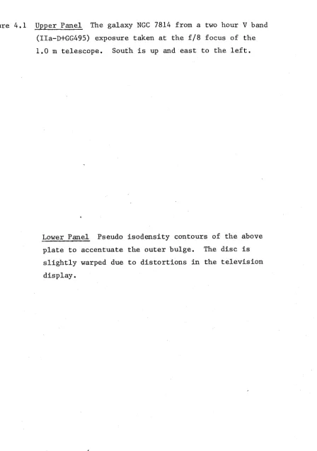
Fit of Grid Power Spectrum to NGC 1404 Photograph of NGC 7814
Minor Axis Luminosity Profile of NGC 7814 in V Two-dimensional Model Fit to NGC 7814 in V Model Fit to Observed Kinematics of NGC 7814 Photograph of NGC 4594
Minor Axis Luminosity Profile of NGC 4594 in V Two-dimensional Model Fit to NGC 4594 in V Model Fit to Observed Kinematics of NGC 4594 Photograph of NGC 7123
Minor Axis Luminosity Profile of NGC 7123 in B Two-dimensional Model Fit to NGC 7123 in B
Rotation and Dispersion Profiles of NGC 7123 4" SW || Fit of Grid Power Spectra to Power Spectra of NGC 7123 Photograph of NGC 4762
Rotation Curve of NGC 4762 6" NW ||
Fit of Grid Power Spectrum to Power Spectrum of NGC 4762
Photograph of NGC 4179
Rotation Curve of NGC 4179 5" NE ||
Fit of Grid Power Spectrum to Power Spectrum of NGC 4179
4.21 Rotation Curve of Ham I 3" E || 151 4.22 Fit of Grid Power Spectrum to Power Spectrum of Ham I 153
4.23 Isophotal Distribution of Ham I in B 155
4.24 V (o)/a vs e Diagram 160
m o max
5.1 Photograph of NGC 128 167
5.2 Rotation and Dispersion Profile of NGC 128 - Major Axis 171 5.3 Fit of Grid Power Spectra to Power Spectra of NGC 128 173
- Maj or Axis
5.4 Rotation Curve and Dispersion Profile of NGC 128 176 -4" E ||
5.5 Fit of Grid Power Spectra to Power Spectra of NGC 128 178 -4" E ||
5.6 Rotation Curve of NGC 128 5" S J_ 181
5.7 Energy-Angular Momentum Plane 185
6.1 Photograph of Thick Disc in NGC 4762 198
6.2 Minor Axis Profile of NGC 4762 200
6.3 Thick Disc Model for NGC 4762 204
6.4 Perpendicular Profiles of NGC 4762 208
2.1 K Index for some King Models 25 3.1 E-W Luminosity Profile of NGC 3379 in B 43 3.2 Comparison of Central Velocity Dispersions of NGC 3379 71
4.1 Parameters of Galaxies Studied 81
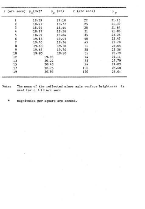
4.2 Minor Axis Luminosity Profile of NGC 7814 in V 86
4.3 Model Parameters for NGC 7814 90
4.4 Minor Axis Luminosity Profile of NGC 4594 in V 102
4.5 Model Parameters for NGC 4594 107
4.6 Minor Axis Luminosity Profile of NGC 7123 115
4.7 Model Parameters for NGC 7123 120
4.8 Rotation Curve of NGC 7123 4" SW || 122 4.9 Velocity Dispersion of NGC 7123 4" SW || 122 4.10 Rotation Curve of NGC 4762 6" NW || 134 4.11 Rotation Curve of NGC 4179 5” NE |j 142 4.12 Rotation Curve of Ham I 3" E || J-42
4.13 Rotation - ellipticity results 158
5.1 Bulge Slit Positions in NGC 128 168
5.2 Rotation Curve of NGC 128 - Major Axis 169 5.3 Velocity Dispersion Curve of NGC 128 - Major Axis 169 5.4 Rotation Curve of NGC 128 4" E || 174 5.5 Velocity Dispersion Curve of NGC 128 4" S || 174 5.6 Rotation Curve of NGC 128 5" S
_L
179C H A P T E R I
INTRODUCTION AND THESIS OUTLINE
1.1 INTRODUCTION
Galaxies are the fundamental building blocks of the universe
and hence have long been objects of great astronomical interest. The
diversity of their forms is great, from elliptical galaxies with a
largely symmetrical smooth distribution of luminosity, to highly irregular
galaxies with no apparent order. Valuable clues to their evolutionary
history can be gleaned from an understanding of their current dynamical
state. For simplicity, it has been natural to look firstly at those
systems which exhibit apparent axial symmetry, i.e. elliptical galaxies
and the bulges of disc galaxies. Detailed observations over the last
few years have allowed us to begin to understand what elliptical
galaxies really are. However, it is only relatively recently that
similar observations have been made for bulges. It is this area which
is the principal aim of this thesis; to gain an understanding of the
current dynamical state of the bulges of disc galaxies. An attempt will
be made to achieve this by a suitable comparison between numerical models
and real observational data. However, before describing the procedures
to be followed in this task, a discussion of previous work in this area
is presented.
1.2 DISCUSSION OF PREVIOUS WORK
The conventional picture of a galactic bulge has been that of an
elliptical galaxy co-existing in the middle of a disc. In view of this
our understanding of elliptical galaxies.
The history of the study of elliptical galaxies can be naturally divided into two epochs. The first, prior to 1975 was hampered by lack of suitable observational material adequately to restrict the range of possible models. The most easily measured observable parameter
was the apparent light distribution. The only kinematical data available were a small sample of central velocity dispersions (Minkowski, 1962; Burbidge et at, 1961a,b,c) which were subsequently shown to be system atically high (Richstone and Sargent, 1972; Morton and Thuan, 1973; Faber and Jackson, 1976). This data alone was unable to discriminate between oblate, prolate or triaxial systems. Nevertheless, models were
constructed assuming oblate spheroids with an isotropic velocity
dispersion. This was prompted by their flattened appearance, and it was believed that collapse of the rotating protocloud proceeded most
rapidly along the axis of rotation (minor axis). Simple models built on this sparse observational background were constructed by Lynden-Bell
(1962), Prendergast and Tomer (1970) and Wilson (1975). These models gave the illusion that the morphology and dynamical properties of
ellipticals were well understood. However, a clue to the incorrectness of these rotationally flattened models was found by Wilson, although he explained this in terms of the inadequacy of the distribution function he chose.
Wilson was expressed in terms of the distribution function of the stellar integrals of motion, with the solution for the model spatial characteristics being well established from the work of many authors (eg. Chandrasekhar, 1943, 1960; Woolley, 1954; Woolley and Robertson, 1956; Woolley and Dickens, 1961; Spitzer and Harm, 1958; Oort and von Herk, 1959; Michie, 1963a,b; Michie and Bodenheimer, 1963; King, 1966).
Other models for elliptical galaxies were also devised, notably those of Gott (1975), involving the dissipationless collapse of the galactic protocloud, and the hydrodynamical models of Larson (1975) with dissipation. However, all of the authors constructing models for
elliptical galaxies did not take account of some important observations which already existed at the time. The most enlightening of these, with hindsight, was the change in position angle with radius of the elliptical
isophotes (eg. Evans 1951, and Liller 1960, 1966). This phenomenon has only recently received attention again, by Williams and Schwarzschild
(1978), Bertola and Galletta (1980) among others, and has two interpret ations: either the galaxy has isodensity surfaces which are spheroids with axes of different orientations, or more probably, these surfaces are triaxial ellipsoids which have the same orientation, but whose axes have different ratios. The isophote twisting is then a projection effect.
The second epoch in the understanding of elliptical galaxies was marked by the observations of Bertola and Capaccioli (1975), Illingworth
(1977) and Schechter and Gunn (1979). They were able to show that the bright ellipticals have rotational velocities typically only about
the classical model in which the flattening is due to rotation alone. The conclusion is that, if the elliptical galaxies are oblate, their flattening is due to a global velocity anisotropy, or, if they do have isotropic velocity dispersions, they must be prolate and rotating end over end. The general case of triaxial ellipsoids is also consistent with this picture.
Given then the long standing view of the similarity in morphology (Sandage, 1961), radial profile shape (de Vaucouleurs, 1959), stellar
4
content, including the L ^ relationship between luminosity L and central velocity dispersion a ,and other basic properties (Freeman,
1975; Faber and Jackson, 1976; Sargent
et at
1977 and Whitmore, Kirshner and Schechter, 1979) between ellipticals and bulges of disc galaxies, it was logical to enquire whether the bulges are also supported in the same way as ellipticals. However, relatively recent data (Kormendy and Bruzual, 1978; Kormendy, 1980b,c ) have permitted these similaritiesto be examined in more detail, with the result that some small but significant differences do exist.
(i) The first of these is the shape of the minor axis luminosity profile. Whereas ellipticals (except possibly for the core regions)
p
are well approximated by a de Vaucouleurs r 4 law (eg. de Vaucouleurs and Capaccioli, 1979) to the limits of available photometry, deviations from
h
the r law are not unknown on the minor axes of galactic bulges.
Notable among these is NGC 4565 (Kormendy and Bruzual, 1978; Jensen and Thuan, 1981; Spinrad
et at>
1978; Hegyi and Gerber, 1977). All these12
steeper than the outer. However, before one concludes that the bulge is showing deviations from the r law, it must be determined whether or not this outer segment is the same dynamical component. In the case of NGC 4565, there is some doubt because of an abrupt increase in colour at the position where the slopes of the luminosity profiles
change (from B-V - 1.0 for r < 60M to monotonically increasing for r > 6Q", Jensen and Thuan, 1981). In addition, the change in slope occurs where the bulge isophotes are most box-shaped. Comparison of M/L values between the inner and outer profiles would be very useful in dis entangling this problem.
Tsikoudi (1977) noted deviations of a slightly different kind in a program of surface photometry of the SO galaxies NGC 3115, 4111 and 4762. As for NGC 4565, she also found an excess over the r law on the minor axis of NGC 4762. However, here at least, this is due to the
presence of the thick disc (Burstein, 1979), shown in Chapter VI to arise naturally where a bulge potential field co-exists with a flat disc potential. In contrast, NGC 4111 shows a deficit of light below the r 4 law, beyond r ^ 15” . This may be caused by the rapid rotation of the bulge which is distinctly peanut-shaped. Finally, it should be noted that there are indeed many bulges which do_ follow the r u law closely; there is a real need to understand how and when the deviations occur.
(ii) There is also an increasing body of evidence suggesting that
elliptical galaxies and even from some bulges of disc galaxies (see Chapter V). Several authors (de Vaucouleurs, 1974; Kormendy and Illingworth, 1980; Hamabe et a Z1980a) have also suggested that in the mean, bulges are flatter than ellipticals, which have a mean shape ^ E4 (Sandage, Freeman and Stokes, 1970). This finding was supported by de Vaucouleurs (1974) who found from a study of bulges in the range Sa - Sc that they were typically E4- E5 compared to E3.5 for ellipticals.
(iii) Without doubt, the most significant evidence against the similar ity of elliptical galaxies and the bulges of disc galaxies comes from recent kinematical observations (Illingworth, 1977; Kormendy, 1980a; Kormendy and Illingworth, 1981, and this work). From observations of
rotation rates in the bulges of edge-on galaxies away from the disc, it is now clear that they are rotating much more rapidly than the bright elliptical galaxies. Moreover, they are qualitatively consistent with the rotating oblate-spheroid models of Binney (1978). Even before these recent observations, it was known that some bulges rotate rapidly,
notably the central region of M 31 (Babcock, 1939; Rubin et aH912>',
Pellet, 1976 and Richstone and Schectman, 1980). Bertola and Capaccioli (1977) had also observed significant rotation in the bulge of NGC 128.
Evidence for bulge rotation also comes from rotation curves on the major axis of SO galaxies, from the inner parts where the bulge dominates the disc (NGC 4762, Bertola and Capaccioli, 1978; NGC 3115, Williams, 1975; Rubin,Peterson and Ford, 1980 , and others). For
has risen to 160 km.s ^ ; this is well in excess of the rotation for most elliptical galaxies. Similarly, for NGC 4762 the major axis is bulge-dominated to a distance of about 10" (Bertola and Capaccioli, 1978), by which the rotation curve has risen to about 80 km.s In summary, even at the very small distances where the disc starts to dominate the luminosity profile on the major axis, the rotation curve velocity measured from the bulge has risen in most cases to values above those commonly seen in ellipticals.
1.3 THESIS OUTLINE
It is now clear that recent data have shown significant photometric and kinematic differences between elliptical galaxies and the bulges of disc galaxies. In particular, there is much evidence for a high degree of rotational support in bulges. Can the observed two-dimensional photo metric and kinematic properties of galactic bulges be adequately modelled via rotationally flattened oblate models? This is the subject of this
thesis. A small sample of edge-on disc galaxies with large apparent bulges was chosen for detailed study and comparison with models. A wide
range of bulge morphologies were selected in an attempt to understand the origin of this range. The data were used as a direct test for the models.
The chapter concludes with an outline of the numerical techniques used in constructing a model of a particular bulge. The necessary dynamical checks on the integrity of the models are also described.
Chapter III describes the observational and data reduction techniques used to acquire the data in a form suitable for comparison with the models. Comparison is also made with standard photometric and kinematic galaxies to test these techniques.
In Chapter IV, models are constructed for three of the six program galaxies with spheroidal bulges, NGC 7814, 4594 and 7123. In general, the agreement between the model predictions and the observations is excellent for both the two-dimensional surface brightness and the kinematics. The dynamical significance of the final adopted models is interpreted with the aid of the V (o)/a v e diagram, wliere V (o),a
m o max m o
and are the maximum rotation velocity of the bulge on the major axis, the central velocity dispersion and the maximum ellipticity of the bulge isophotes respectively. The remaining three galaxies in the sample, NGC 4762, 4179 and Ham I are also discussed here. The mass-to-light ratios are computed for those galaxies with a fitted model.
Chapter V contains a discussion of the cylindrically rotating bulges. There is a growing body of evidence to suggest that, kinematic ally, bulges fall into two distinct classes, the cylindrically rotating and non-cylindrically rotating bulges. It is suggested that the nature of the rotation is revealed by the morphological form of the bulge; the box and peanut-shaped bulges are all cylindrically rotating and
for galaxy formation are also discussed in terms of the density distribut ion of stars in the energy-angular momentum plane. Finally, a possible correlation between the presence of a halo globular cluster system and the bulge morphology is also discussed.
In Chapter VI, the dynamical origin of thick discs is investigated, from the assumption that they result from the response of the bulge
DYNAMICAL MODELS OF GALACTIC BULGES
2.1 INTRODUCTION
In this chapter a set of dynamical models for the bulges of disc galaxies are described. The models are axisymmetric and are based on a distribution function of the two isolated integrals of motion, energy and angular momentum. The bulge models have non-zero total angular momentum, and are spatially truncated by an energy cutoff.
The theory of the models and the assumptions on which they are based are discussed in section 2.2. The numerical schemes for constructing the models are detailed in section 2.3. In section 2.4, two numerical checks are described for testing the models and
section 2.5 briefly discusses the projection of the models on to the plane of the sky for comparison with observation. Finally, in
section 2.6, the assumptions on which the models are based are reiterated and the observational data required to investigate their validity discussed.
2.2 THE MODELS
Recent observations (Bertola and Capaccioli 1975; Illingworth 1977; Schechter and Gunn 1979) have shown that elliptical galaxies are probably not simple oblate systems flattened by rotation alone
function on the isolating integrals of the motion and then solves for the corresponding stationary density distribution and gravitational potential fields. (This is not the only way that one could proceed. Lynden-Bell (1962) demonstrated that one can in principle find a distribution function for any axially symmetric system, given its density distribution. This procedure to date has been not much used, because of technical difficulties.)
The disc of a disc galaxy provides a significant contribution to the total (i.e. bulge + disc) potential, and should not be ignored. In this study the disc potential is represented as a static external potential. The bulge is modelled in a self-consistent manner with every bulge star moving in the collective potential field set up by the stars of the bulge itself plus imposed potential of the disc. The inclusion of the disc was found to model more realistically the
potential in which the bulge stars move (see Chapter VI). A further refinement to the models would be to include the potential field generated by the massive halo of the type invoked by Ostriker, Peebles and Yahil (1974) to account for the flat rotation curves of
I n t h e a b s e n c e o f a f o r m a t i o n t h e o r y f o r g a l a x y f o r m a t i o n
r i g o r o u s e nough t o p r e d i c t r e l i a b l y t h e e x p e c t e d d i s t r i b u t i o n
f u n c t i o n , t h e c h o i c e r e m a i n s l a r g e l y a r b i t r a r y . T h i s l e a d s t o a l a r g e
number o f p l a u s i b l e d i s t r i b u t i o n f u n c t i o n s s a t i s f y i n g t h e c o l l i s i o n l e s s
B o l t z m a n n e q u a t i o n . I n v i e w o f t h i s and t h e s u c c e s s i n a p p l y i n g
Ki n g m o d e l s ( Ki ng 1966) t o g l o b u l a r c l u s t e r s and some e l l i p t i c a l s , i t
i s a ss um ed t h a t t h e d i s t r i b u t i o n f u n c t i o n f o r t h e b u l g e s o f d i s c
g a l a x i e s h a s t h e s e p a r a b l e f o rm :
f ( E , J ) = a [ e x p ( - B E ) - e x p ( - ß E ) ] e x p ( y J ) ( a )
o
w h e r e E<Eq = c o n s t a n t and a , B a n d y a r e c o n s t a n t s . The two i n t e g r a l s
o f m o t i o n , E and J , a r e t h e e n e r g y p e r u n i t mass and t h e c omponent o f
a n g u l a r momentum p e r u n i t m as s p a r a l l e l t o t h e a x i s o f s y mm et ry . I n
s p h e r i c a l p o l a r c o - o r d i n a t e s ( r , 0, cj)) w i t h c o r r e s p o n d i n g v e l o c i t i e s
v » v q> v » t h e s e i n t e g r a l s a r e :
r 0 4>
E = ^ ( VJ +V0+V| ) + U ( r , 0 ) ,
an d J = r s i n 0 v ^ .
<P
U ( r , 0 ) i s t h e t o t a l g r a v i t a t i o n a l p o t e n t i a l a t ( r , 0 ) . Lowered
M a x w e l l i a n d i s t r i b u t i o n f u n c t i o n s y s t e m s w i t h no mean r o t a t i o n
( i . e . y=0) a r e Ki ng m o d e l s .
The d e n s i t y a t any p o i n t i n t h e m odel i s f o u n d by i n t e g r a t i n g
f ( E , J ) o v e r v e l o c i t y s p a c e , i . e .
P ( r , 0 ,U) = f ( E , J ) d v d v . d v .
r 0 4> (b)
Th e n a s e l f - c o n s i s t e n t model i n w h i c h e a c h s t a r moves i n t h e s mo ot he d
c o l l e c t i v e g r a v i t a t i o n a l f i e l d o f a l l t h e o t h e r s t a r s i s c o n s t r u c t e d
Most of the numerical effort goes into finding the solution to this equation.
Substituting equation (a) into equation (b) and performing the and Vg integrations, one obtains:
p ( r
,e,u)
2ttuv c
[exp(-3£) + 35exp(-3EQ)-l] exp(yrv^sin0)dv^ -v
c (d)
where £ = + U and v = (-2U) is the local cutoff velocity.
<p c
Thus U = 0 defines the boundary of the model and externally to this, p(r,0,U) = 0 for all U(r,0)>O. The constants in equation (d) are now eliminated by introducing dimensionless variables with suitable scale
factors.
Aside from those cases where there is no chance of confusion, let an asterisk subscript distinguish dimensional quantities from their dimensionless equivalents. In this notation, equation (c) becomes:
rP
W
r*e)
= 4 * G P * < r * . e . V .Now make the change of variables: W = -3U^,p
and r = r^/£^, so V2 = £2V2 . Poisson’s equation can then be rewritten as:
V2W ( r ,0) = -Xp(r,0,W)
where X = (4ttG£23Pqä)/p . The zero subscript refers to the origin. The scale length factor Z can be made equivalent to the core radius, r , as defined by King (1966) if
c
X = 9/p .
o
Thus only relative values of the density are needed and Poisson’s equation in final form becomes,
v
fC
[exp(-0O + B£exp(-0E )-l] exp (y r v s i n )dv
J o * cp 0 <p
-v c
V
[C
[exp(-3? ) + 3C exp(-BE )-l]dv
J
O
O
0
({>
- V
c
Let also q
h
v , and y = r <f> c
2
y ; then in its fully expanded dimensionless form, equation (e) becomes,
V W(r,0) = -9 [exp(-q -fW) + (n —w) — 1 ] exp(yqrsin0)dq
-W (f)
[exp(-q2+W ) + (q2-W )-l]dq
o o
-W
where W, y, q and r are all dimensionless.
Two parameters are thus required to specify uniquely the dimensionless bulge model; they are the central bulge potential W
o and the rotation parameter y. In this form, the dimensionless potential is the same as that used by King, i.e. King models are produced when y = 0 (non-rotating). This was one of the properties used to test the models - see section 2.5.
The following observables and moments of the velocity dispersion were calculated from the converged model.
(1) velocity dispersion:
<v > = < V >
r 6 exp(-q2+W) + (q2 —W ) - — --- 1 exp(yrqsin0)dq -W
, 2 2
and <vf> = — [exp(-q2+w) + (q2—W) -1] exp(yrqsin0)dq - W
H
<v > = ( 2 / 3 p ) <f>
h
-w
h.[ e x p ( - n 2+w) + ( n 2- w ) - l ] e x p ( y r s i n ö r i ) . pdp
( 3 ) p r o j e c t e d r o t a t i o n a l v e l o c i t y :
00
V = v<v >pdx
Z 9
— 00
w h e r e Z i s t h e p r o j e c t e d s u r f a c e b r i g h t n e s s and v i s t h e d i r e c t i o n
c o s i n e , an d x i s a l o n g t h e l i n e - o f - s i g h t .
( 4) p r o j e c t e d v e l o c i t y d i s p e r s i o n :
° 2 = i it.- l <v?>pdx - V2l
w h e r e t h e s u mm at io n c o n v e n t i o n i s i n t e n d e d .
Of p a r t i c u l a r i n t e r e s t t o t h e d e g r e e o f r o t a t i o n a l s u p p o r t i n
a g a l a c t i c b u l g e i s t h e r u n o f V ( r ) /cj w i t h r a d i u s a l o n g t h e m a j o r
a x i s , w h e r e a i s t h e c e n t r a l v e l o c i t y d i s p e r s i o n . ( s e e C h a p t e r IV) o
From e q u a t i o n s ( g) and ( h) e v a l u a t e d on t h e m a j o r a x i s , t h i s q u a n t i t y
c a n b e f o u n d f r o m ,
V ( r )
„ / \ , v<v >pdx Z ( r ) J <J) M
1
Z ( r = o ) <v >pdx r
( i i ) The D is c
As m e n t i o n e d e a r l i e r , t h e d i s c o f a d i s c g a l a x y c o n t r i b u t e s
s i g n i f i c a n t l y t o t h e p o t e n t i a l an d i t s e f f e c t h a s b e e n i n c l u d e d i n
t h e s e m o d e l s a s a n e x t e r n a l l y i mp os e d p o t e n t i a l . As w i l l b e d i s c u s s e d
i n C h a p t e r V I , t h e a d d i t i o n o f a d i s c p o t e n t i a l f i e l d i n t h e m o d e l s
i s a more r e a l i s t i c a p p r o x i m a t i o n t o t h e d y n a m i c a l e n v i r o n m e n t i n
w h i c h t h e b u l g e c o - e x i s t s , and a s a r e s u l t o f t h i s , t h e f i n a l m o d e l s
w e r e f o u n d t o b e i n b e t t e r a g r e e m e n t w i t h t h e o b s e r v a t i o n a l d a t a .
A n o t h e r m o t i v a t i o n f o r t h e i n c l u s i o n o f a s t a t i c d i s c
Let U, and U, be the potential of the bulge and disc respectively
b d
at any point in the model.Then
V 2 ( U , + U J = 4ttG
b d f (^c2+U, +U ,, b d J) d 3c + 4ttG Paj
where and p^ are the corresponding bulge and disc densities at this
point and c are the velocity components. The disc potential field
satisfies Laplace's equation outside the disc and Poisson's equation
within, i.e.
V 2U, = 0
d outside disc
and V 2U, = 4rGpj
d d inside disc.
Thus equation (h) may be written as:
V2IL = 4ttG
b f(^c2+UL+ U jSJ)d3cb d
This means that the bulge model, in the external potential field of
the disc, can still be solved self-consistently; the only modific
ation required is that the energy integral of the bulge include the
total (bulge + disc) potential. In view of their analytic simplicity,
the disc models of Miyamoto and Nagai (1975; hereafter MN) were
used. The disc potential field U^(r,z) is given in cylinducal
co-ordinates (r,z) as:
U d (r,z)
G M ,
___________ d__________
{r2 + [a + (z 2+b 2)^ ]2
(i)
where is the mass of the disc, and a and b are scale lengths in
the equatorial and vertical directions respectively. This
axisymmetric potential field is free from singularities, differentiable,
and tends to the Keplerian potential for large r and z. From
Poisson's equation using this potential field, MN showed that the
P ( r , z ) 4
tt
( r 2+ [ a + ( z 2+ b 2) 2] 2 } ^ ( z 2+ b 2 ) ^
We now r e q u i r e e q u a t i o n ( i ) i n t h e same d i m e n s i o n l e s s u n i t s
a s t h e b u l g e . U s i n g t h e same n o t a t i o n a s b e f o r e , t h e d i m e n s i o n a l
p o t e n t i a l a t t h e o r i g i n i s ,
GM
u d ■ V ° - 0) ( a+b)
G ( a+b)
w h e r e M, = p ° r 3y, .
b b c b
pb r c \
The q u a n t i t y y^ i s d e f i n e d a s :
r ft Pb
— rr 47TS2d s .
P-L
o b
w h e r e r i s t h e t i d a l ( b o u n d a r y ) r a d i u s o f t h e m o d e l . As b e f o r e and
f o l l o w i n g K i n g , t h e c o r e r a d i u s r ^ i s d e f i n e d b y ,
47rG3r 2p° = 9
c b ( 3 = 2 j 2 i n K i n g s n o t a t i o n )
i . e . ß
4TTGr 2 p £
c b
I n t h e same d i m e n s i o n l e s s u n i t s a s t h e b u l g e , t h e d i m e n s i o n l e s s d i s c
p o t e n t i a l i s W^ = -3U^ an d t h e r e f o r e ,
- 9 G . Md
4 r G r 2p^
c b ( a+ b) “ b
- 9 y , r
b c Ma
4tt ( a+b) “ b
o,. 3,
w h e r e a and b h a v e b e e n r e w r i t t e n i n d i m e n s i o n l e s s u n i t s a s a / r and c b / r ^ r e s p e c t i v e l y .
The f i n a l f or m f o r t h e d i m e n s i o n l e s s c e n t r a l d i s c p o t e n t i a l
i s t h e n :
M,
ttO _ -9Q
d 4tt ( a + b ) w h e r e Q = Ih
redistribution of the mass in the bulge due to the presence of the disc will alter y . Instead, a value is assigned to Q, W° and Y, the
b b
model computed, y calculated a posteriori and M,/M retrieved from
b d b
M^/M^ = Q/ ^ b * ■*'n P r a c t i-c e > the values given to y^ for a suitable input value of Q are similar to those derived by King as a function of central potential for his globular cluster models. If this is done, then the ratio of the input to output mass ratio does not vary by more than a factor of two.
With the addition of the disc to the bulge models, the number of free parameters now required to uniquely specify the model has increased to five i.e. W 0, Y, a, b and Q. The first two parameters
b
define the bulge and the remaining three the disc. The disc to bulge mass ratio enters implicitly through Q.
To summarize, the models presented above are intended to
represent the present dynamical state of the bulges of disc galaxies. The models are tidally truncated and are flattened mainly by
rotation: the externally imposed disc potential also contributes to their flattening. To test these models, they must be compared against observed two dimensional light distributions and kinematical properties of real galaxies. Before this is done, the numerical techniques used in calculating the models are detailed.
2.3 NUMERICAL TECHNIQUES
The main thrust of the numerical techniques was to develop an algorithm for solving the dimensionless Poisson equation (e). To this end, it has been popular to express the density and potential
functions in terms of Legendre series (cf PT and Wilson) i.e. 2N-2
W(r,0) = y a (r)P (cos0) n n
u
n n n=oThe summations need only extend over even values of n due to the
equatorial symmetry of the models. The value of N is chosen in
accordance with the desired accuracy of the numerical solution. Clearly
as the models become flatter (y i ncreasing), a greater number of terms
are required in the expansion.
Using these expansions and the boundary conditions
W(r=O,0) = W , 3W/3r
o r=o 0 and 3W/3r f - K ß 0, PT showed that the solution to equation (e) is,
W(r , 0) = W + X
o sb (s)ds - —o r s 2b (s)dso
-X Z
P (cos0) n
n=2 2n+l
1_r 1
s b (s)ds + — —
n n+i sn + 2 b (s)dsn (j )
This expression was evaluated on a polar grid in r and 0. The divisions
in r were variable so that a fine grid was used near the centre where
the density gradient is large. To avoid unnecessary interpolation in
the 0 direction, the rays were chosen to coincide with the 0^ values
defined by the Gauss-Legendre integration (see b e l o w ) . This differs
from the otherwise similar procedure of van Albada and van Gorkom
(1977; hereafter AG) who used an evenly spaced grid in 0.
The two integrals in the summation of equation (j ) were
evaluated using the recurrence relations derived by AG. At any
point (r^»®^) t*ie (r >0) grid they write,
s1 rb (s)ds + --7—
n n+! sn+2b (s)ds = F (r.) + G (r.) .n n 1 n 1
Hence the value of F at r. is related to the value at r. by,
n 1-1 1
F (r
)
n 1-1 i-- s1 nb (s)ds + i—
w
•F (r. ) n l-i
i - i
l j V
Pi ~ri-i)
•bn (ri-%> + W l.1+(ri-i)/rr
where r i_i^ = il(r i_ 1+ r i) . A starting condition of F (r ) = 0 enables
F to be evaluated for all values of r and n. n
A similar recurrence relation also exists for G,i.e.
Gn (ri+ 1 >
I l+n 1+R
1 + n ( r * - r . 2 )
i+i i
-.b (r ) + G (r .)
n 1+^ n l
where R = r./r., . The starting condition is G (r ) = G (0) = 0.
l i+i 0 n i n
All that remains to calculate are the b . These are evaluated using n
either a 12 or 24 point Gauss-Legendre quadrature over cos0 i.e.
b n (r) = %(2n+l)
I
w k P(r,ek )Pn (cos0K), k=iwhere m = 12 or 24. The weights w k have been taken from Davis and
Polonsky (1964). In terms of the F and G recurrence functions, the
n n
n=0 term of equation (j ) is,
F (0) - F (r) - G (r)
0 0 0
The numerical scheme for computing a self-consistent stationary model
is now clear. An initial guess is made for the bulge density
distribution at every point in the grid. This allows the calculation
of the density expansion coefficients b (r). Next, the recurrence n
relations are used to compute the potential field corresponding to
this density field, from P o i s s o n ’s equation. The contribution from the
disc potential at each point is added,and a new density distribution
calculated by integrating the distribution function. This process
was repeated until convergence occurred. Convergence was assumed
to occur when the difference in density at every grid point in the
model between successive iterations was less than 0.1 percent.
minor a x i s ) . The total CPU time required using the Australian National
University Univac 1100/82A computer was typically less than five
minutes. Longer times were required for rapidly rotating models.
2 . 4 NUMEPvICAL CHECKS
Several numerical checks were made to confirm the accuracy and
dynamical integrity of the models. The simplest of these was
afforded by comparing spherical (King) models without a disc,
(computed in the generalised three-dimensional grid) with those
published by King. The models were indistinguishable within the range
of central potentials consistent with the observed range of central
concentrations, from the least concentrated globular clusters to the
elliptical galaxies i.e. ~ -3 to -13.
A second more stringent test was the virial theorem, T/ft = -%,
where T and ft are the total internal kinetic and potential energies
respectively. These are easily shown to be,
a (s)b (s)
v n n
k P0 (2k+1) .4irs2ds
-b (s)
-. 4irs2ds
and — (2<v 2> + <v , 2>)dcos0.2iTS2ds
P_ r <t>
in dimensionless units. The (non zero shifted) potential at
infinity, W is
r
it W + A
o s b (s)dso
where r^_ is the maximum radius of the boundary.
For the rotating models without a disc, the virial theorem was
found to be satisfied to better than 0.1 percent in all cases. However,
a disadvantage in using the virial theorem as a dynamical check is that
parts of the model. An independent point to point check in the model
is the most desirable, so the stellar hydrodynamical equations (HEs)
were used as a check.
In spherical polar co-ordinates the _r component of the HEs,
from Ogorodnikov (1965) is
3<v > . <v >9<v > . . <v >9<v > ,
r + r r + 1 6 r + 1
9r 96 r sin 6
<v >9<v > <f> ___
96
2 ' 1
- — (<v > 2+<v > 2) 1---<v > 2 + <v ><v > co-t0
H--r 0 6 r r r 0 p
3(po ) rr 3r
, 1 3(p0re) ,
r 90 r sin 0
1 3(° r ^
36 - + %
+ r0 cot0 3W
where a 1 (vi~ < v i>)(v -<v^>) f ( E ,J ) d 3c . ij P
It is easy to show that a
delta. The models are stationary (9/91 = 0) and axisymmetric .. = 6.. a., where 6.. is the Kronecker
ij ij ij iJ
(9/96 = 0)* Also <v^> and <v^> are zero and therefore the _r component
of the HEs is reduced to
9p<v 2> p<v 2> p<v 2>
r r _ 6
V '
_3W9r (k)
since a ( v .- < v . >)2f (E , J) d 3c = —
x l 7 p v ^ 2f(E,J)d3c <v. >l
Similarly the _0_ component of the HEs is
9<Vq> <v r>3<ve> <V Q> 9<ve> <V6> ^< V 0> <v ^ > 2cot0 3t
<v ><v >
+
90
+
—
S- + ±
r p
rsin0 96
3pa
r 3pore 1 3pgee 1
9r r 90 rsin0 96
66
PG,,COt066 __
3 , paeecote n + 2 p°r0 + ---- —
tan0 3p<v 36
p<v,2> p<v 2>
—
i—
+ — J—<v >
4> _ tan6 3W r “ r "ae
(
1)
The 4> component vanishes in an axisymmetric model. Equations (k) and (1) were applied at every grid point along the major and minor axes of
the model. This is a better check for the outer parts of centrally concentrated models than the virial theorm.
To illustrate the accuracy of a model, a moderately concentrated rotating system was constructed with (W^,y) = (-8,0.3). Figure 2.1 shows the radial distribution of error in the HE's, normalised to the potential gradient along the major and minor axes. To a radius of 0.9r^_, the error does not exceed 0.2 percent. The morphology of the radial error distribution also illustrates well where the greatest need is required for a finer radial grid. This in fact could be used to force the radial grid to follow the density gradient in the model. This would ensure a more constant error, independent of central
concentration and position in the model. For all the computed models, with or without discs, the error derived from the HEs along the major
and minor axes did not exceed one percent.
In summary, the models are believed to be dynamically accurate within the domain of input parameters commensurate with real physical
systems.
2.5 PROJECTION
To compare the models with real observations, the models must first be projected on to the plane of the sky. In doing this the models were assumed to be transparent and have a constant mass to
light ratio. The projected surface density E, was computed from the
integral
E pdx
(m)
CD 42 4-1 o ■ u X CD co •H i—I CO
a
o e c o •H 4-1 CO 3 a " <U e •H u o u u CL) CL) bO cO 4-J a 5-4 Q) a CL) 4 2 H 4-1 e o •H XI cO 5-4 bO rH CO •H 44 o a CN a) 5-i 2) bO •H PH CO • H 4 2 4-1 CN A > 5-i V I<— < 1 Q _
II
c
a) 5-i a> 4-1 O a) x 2> 4 J •H X a cO (2 O •H4- 4 21 4 3 •H 5- 1 4-1 CO •H X a ) 42
4- 4
O 42 CO CO CD > 5- 1 2) U X CL) rH rH 0 ) 4 2 CO i— I o £ 4-4 CL) 42 H 5h O 5-( 54 0 ) a •H a) CO CO 0 ) 54 u p •H I—I cO CJ o r— I CL) 42 H CO 0) X CÜ M o 52 • H
e
X 52 cO • x cO e 44 54 < r o X vO 54 <3 e o 54 4 4 b O5
CO cO CD 54 U (2 •H 54 (2 •H X •H 54 bO a) 42 44 o 44 CD 23 X CO •H 4 4 O 44 CO o e 54 0 ) > O 44 52 0 ) U 54 CD 2 5 O 52 cO 42 44 CO CO CD I—I CO •H 54 O 54 54 0) CD 42 E-4 CD 42 44 bO 52 O i—I cO 54 O 54 54 CD*--4 44 • 54 O r o
<? 'o
00
o
<
£
>
Ö
Ö
CNJ
ö
o
ö
PO CNI O
Ö Ö CD Ö
r\i CD I
jo jj e o
/0
o
I
PO
CD
a fine grid in the models came in the projection in that equation (m)
could be used directly. In other projection schemes (e.g. Wilson
1975), the above integral could not be applied directly due to a much
coarser grid in regions of high spatial density gradient. Another
advantage of using equation (m) directly in a fine grid is the speed
of the projection code. The average CPU time per model was about
15 seconds. As a numerical check on the accuracy of the projection,
triaxial ellipsoids were projected and compared with their theoretically
projected values. The agreements were excellent.
2.6 SOME MODEL PROPERTIES
Many of the model properties may be conveniently described in
the central potential - rotation parameter (W°,Y) plane. The first b
problem to be encountered when constructing a model for a particular
galaxy is the initial choice of W° and Y. One method by which these b
quantities may be estimated is to construct a variable which will
parametrize the "concentration" of the model and galaxy. Then, by
measuring this quantity from the data, a starting (W^,Y) pair may be
interpolated from the (W°,y) plane. The effectiveness of this b
parameter is greatest if it can be computed quickly and accurately.
It must also be sufficiently sensitive to changes in concentration
over the range of interest in astrophysical situations. Consider a
concentration index K defined by
<r>‘
where <r> prdr
/
pdrand <r >2 p r 2dr
/
p d r .This particular concentration index lies within the range K < 3/1+ .
index K for some King models (y = 0).
TABLE 2.1
K INDEX FOR SOME KING MODELS
Ki
log c K2.5 0.590 0.576
3.0 0.672 0.563
4.0 0.840 0.532
5.0 1.029 0.490
6.0 1.255 0.437
7.0 1.528 0.367
8.0 1.833 0.283
9.0 2.119 0.199
10.0 2.350 0.135
12.0 2.739 0.059
It can be seen that K has the desirable property of being monotonic with concentration and reasonably linear over the above range of
central potentials.
Using this definition for K, a grid of models was then constructed with different values of W° and y. These allowed loci
b
of constant concentration to be drawn in the (W°,y) plane, shown in b
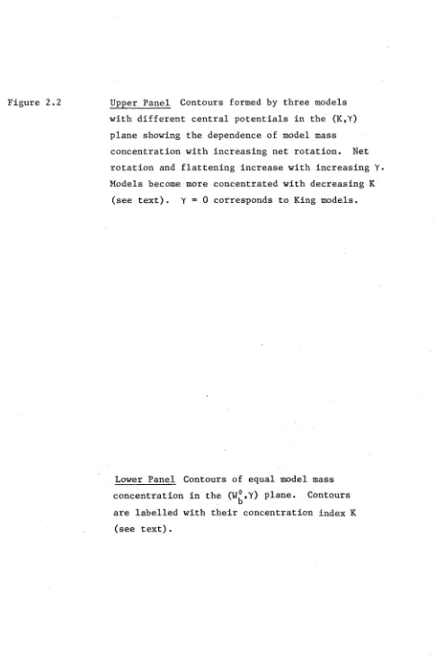
the lower panel of Figure 2.2. A series of models with constant central potential are shown in the (K,y) plane of the upper panel of Figure 2.2. The most striking result from this figure is that the concentration of the models is nearly independent of their initial W° values for y greater than about 0.6 (corresponding to a flattening
b
of nearly E6) . However, the bulges of most disc galaxies in the (K,y) plane do not lie in this region of ambiguity, but have 0 < y < 0.6.
Figure 2.2 Upper Panel Contours formed by three models with different central potentials in the (K,Y) plane showing the dependence of model mass
concentration with increasing net rotation. Net rotation and flattening increase with increasing Y. Models become more concentrated with decreasing K
(see text). Y = 0 corresponds to King models.
Lower Panel Contours of equal model mass concentration in the (W°,Y) plane. Contours
b
[image:40.547.46.530.68.804.2]-10.0
Y
- 10.0
0.275
The models presented above were constructed to represent
the current stationary dynamical state of the bulges of disc galaxies. They assume the bulges are oblate and flattened mainly by rotation. The distribution function is truncated by an energy cutoff, and has an angular momentum term which gives non-zero net rotation. The only way to test the assumptions on which this model is based is to
compare the structure and internal kinematics of the resultant models with the real data. To do this the following observational material
is required:
(i) accurate two-dimensional surface brightness maps of the bulges of edge-on disc galaxies,
(ii) spatial mean rotation profiles in the bulge and (iii) spatial velocity dispersion profiles in the bulge.
C H A P T E R I I I
OBSERVATIONAL TECHNIQUES AND DATA REDUCTION
3.1 INTRODUCTION
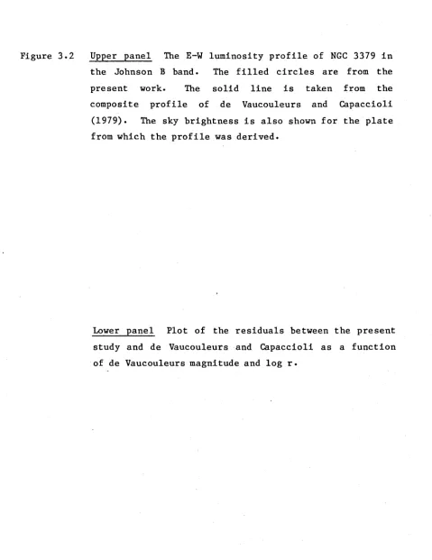
This chapter describes the observational and data reduction techniques used to test and constrain the bulge dynamical models of Chapter II. A program of two-dimensional surface photometry for four suitable candidate edge-on SO and early type disc galaxies was a major part of the observational work. Section 3.2 describes the acquisition and reduction of the photoelectric photometry and in section 3.3 the photographic photometry is discussed. An external check on the surface photometry was made by inclusion in the sample of galaxies, the luminosity distribution standard NGC 3379. This galaxy was selected for this purpose by the Working Group on Galaxy Photometry of IAU commission 28 (IAU Trans., XIB, 304). The photometry is compared in section 3.4.
Observations of rotation and velocity dispersion in a sample of SO’s were made using the Image Photon Counting System (IPCS) of the 4m Anglo Australian Telescope (AAT) at Siding Spring Observatory. The procedure for velocity measurement is described in section 3.6 and in section 3.7 I discuss the technique used for the derivation of velocity dispersion.
3.2 PHOTOELECTRIC PHOTOMETRY
('i) Acquisition
V : 2 mm Schott GG495
B : 2 mm Schott BG12 + 1 mm Schott GG385 and U : 1 mm Schott UG1.
The detector was a dry-ice cooled 1P21 photomultiplier tube with an SSR pulse amplifier and the Mt Stromlo General Purpose Scaler (GPS). The GPS is a computer controlled photon counting system; the user defines the sequence of instructions to be executed through a BASIC control language on a PDP 11/34 computer, and outputs the data to data cassette or floppy disc.
The photoelectric observations consisted of a series of long strings of short integrations as the photoelectric aperture drifted across the galaxy in an east-west line. Each of these strings was stored in memory as an array and co-added to similarly repeated strings. All observations were made using an aperture of 1.36 mm diameter which corresponds to 29.0 seconds of arc. The aperture was centred visually on the nucleus of the galaxy to be observed and the telescope slewed to the west a distance of at least
5Ü25* The ^25 values were taken from the Second Reference Catalogue of Bright Galaxies (RC2) (de Vaucouleurs, de Vaucouleurs and Corwin 1976). For galaxies with no available value (NGC
variable frequency oscillator to suit the integration time per channel and the total distance to be traversed by the drift scan. At the completion of each drift scan the data was displayed on a Tektronix 4010 terminal, with the observer having the option of either accepting or rejecting the last scan. If accepted, the scan was added to the previous scans and the average displayed. A completed observation was typically the average of 10 scans each of 600 channels, which was then saved on data cassette for later evaluation and reduction. This gave a total of approximately 1500 counts per channel per second integration in B. The drift rate was also adjusted to give about five channel integrations per aperture. Approximately every two hours throughout the night, four to six standard stars were observed: these were used for the determination of the transformation coeficients. Each standard star was observed in the U, B and V passbands with an integration period of ten seconds. This sequence was repeated after a similar observation of nearby sky.
Cii) Reduction
then applied to the clipped data to determine the sky count level. This fitted sky was then subtracted from the cleaned data to produce a sky subtracted scan in preparation for transformation on to the appropriate magnitude scale for the filter used. In all cases the sky was fit to better than 0.5%. The accuracy of the fit was limited by sky photon noise and variable extinction between each averaged scan. A linear fit was also assumed. The transformation coefficients obtained from the standard stars measured before and after each completed set of drift scans were then computed using mean extinction coefficients. The adopted extinction coefficients were:
Ky = 0.16 magnitude.airmass ^
Kg_y = 0.12-0.04 (B-V) magnitude.airmass ^ and k u-B = 0*36 magnitude.airmass ^ •
The coefficients adopted for the drift scan transformations were taken as the average of the standard star coefficients obtained before and after each drift scan set. Once the sky subtracted drift scans were transformed on to a magnitude scale, the drift scans were ready to define the magnitude zero-point for the photographic photometry.
3.3 PHOTOGRAPHIC PHOTOMETRY
(i) Acquisition
plate-filter combinations used to define the B and V passbands were: B = lla-O + GG385,
V = Ila-D + GG495.
All B and V plates were hypersensitized before exposure. After an initial soaking for 15 hours in nitrogen at room temperature, the plates were flushed with hydrogen every hour for a total of seven hours. Tests were carried out prior to exposure to check for plate fog and speed. Calibration for the plates was provided by use of a spot sensitometer, housed in the 1.0 m telescope building. The sensitometer was constructed by G. de Vaucouleurs and consists of a stack of 15 tubes, each with an entrance aperture of well determined size. All exit apertures are of identical size. This produced a set of three rows of five spots covering a range in surface brightness of 3.85 magnitudes. Uniform illumination at the base of the tubes is provided by an opal glass diffuser, illuminated by a tungsten lamp light source located approximately 50 cm below the diffuser. The calibration spots were exposed at the same time as the telescope exposure, on a separate plate from the same box and hypering batch as the telescope plate. Spot exposure times were always within 20% of the telescope exposure times and in as similar temperature and humidity conditions as possible. The sensitometer room was well ventilated to the outside air, so conditions were similar to those in the dome at the time of exposure. Both plates were hand processed simultaneously in D19 and 20°C for five minutes, within 18 hours of exposure.
Cii) Reduction
(a) Microphotometry
density increments of 0.00125 density units. A large degree of flexibility in the measuring procedure was possible using the PDS control program FORNAX written at Mt Stromlo for the PDS. The raw PDS data was written directly to nine track magnetic tape for further reduction.
To ensure that the PDS measuring runs were as similar as possible, each run was treated as a photometric session. The 12-bit configuration of the PDS enabled all runs to be performed in the density mode. Constancy in the set-up procedure was ensured by:
(i) allowing a warmup period of at least two hours,
(ii) using a plate of clear glass, the same thickness as the exposed plates to set the PDS voltage and density controls, and,
respond to rapid changes in plate density and hence input signal. Each PDS session involved the following set of measurements; the repeated set-up for different apertures being necessary since the PDS "sees" the plate with different f ratios for different apertures. For this reason, the two aperture sets were tied together by scanning the calibration spots with both apertures.
(i) set up PDS with the 25 pm^ aperture, (ii) scan the calibration spot plate,
(iii) scan two adjacent areas (61x61 pixels) of fog in each corner of the galaxy plate,
(iv) scan the galaxy frame,
(v) rescan the fog spots in each corner, (vi) set up PDS with the 125 pm^ aperture,
(vii) scan the same fog spots (13x13 pixels) in each corner of the galaxy plate,
(viii) scan the sky frame,
(ix) rescan the fog spots in each corner, (x) scan the calibration spot plate.
All the above data was written on to magnetic tape for later reduction. The drift in the PDS photoelectric system observed over several hours of measurement was less than four PDS units (0.001 density units). Constancy between sessions was excellent.
(b) Spot Calibration