The relationship between Neogene dinoflagellate cysts and global climate dynamics

This is a repository copy of

The relationship between Neogene dinoflagellate cysts and

global climate dynamics

.

White Rose Research Online URL for this paper:

http://eprints.whiterose.ac.uk/125411/

Version: Accepted Version

Article:

Boyd, JL, Riding, JB, Pound, MJ et al. (4 more authors) (2018) The relationship between

Neogene dinoflagellate cysts and global climate dynamics. Earth-Science Reviews, 177.

pp. 366-385. ISSN 0012-8252

https://doi.org/10.1016/j.earscirev.2017.11.018

Crown Copyright © 2017 Published by Elsevier B.V. This manuscript version is made

available under the CC BY-NC-ND 4.0 license

https://creativecommons.org/licenses/by-nc-nd/4.0/

eprints@whiterose.ac.uk https://eprints.whiterose.ac.uk/

Reuse

Items deposited in White Rose Research Online are protected by copyright, with all rights reserved unless indicated otherwise. They may be downloaded and/or printed for private study, or other acts as permitted by national copyright laws. The publisher or other rights holders may allow further reproduction and re-use of the full text version. This is indicated by the licence information on the White Rose Research Online record for the item.

Takedown

If you consider content in White Rose Research Online to be in breach of UK law, please notify us by

1

The relationship between Neogene

1

dinoflagellate cysts and global climate dynamics

2

Jamie L. Boyd

_{, James B. Riding}

_{, Matthew J. Pound}

_{, Stijn De Schepper}

_{, Ruza F. Ivanovic}

_,

Alan M. Haywood

_{and Stephanie E.L. Wood}

1_{School of Earth and Environment, University of Leeds, Woodhouse Lane, Leeds LS1 9JT, UK} 5

2_{British Geological Survey, Environmental Science Centre, Keyworth, Nottingham NG12 5GG, UK} 6

*jbri@bgs.ac.uk 7

3_{Department of Geography and Environmental Sciences, Northumbria University, Newcastle} 8

upon Tyne NE1 8ST, UK 9

4_{Uni Research Climate, Bjerknes Centre for Climate Research, PO Box 7801, N-5020 Bergen,} 10

Norway 11

5_{Department of Animal and Plant Sciences, University of Sheffield, Western Bank, Sheffield S10} 12

2TN, UK 13

14

Key Words: dinoflagellate cysts; global distributions; Neogene; palaeoclimate; palaeoecology; 15

palaeotemperature 16

17

Abstract

18

The Neogene Period (23.03 2.58 Ma) underwent a long-term, relatively gradual cooling trend, 19

culminating in the glacial-interglacial climate of the Quaternary. Palaeoclimate studies on the 20

Neogene have provided important information for understanding how modern patterns of 21

2 change. Here we use a newly created global database of Neogene dinoflagellate cysts (the Tertiary 23

Oceanic Parameters Information System - TOPIS) to investigate how dinoflagellate cysts recorded 24

the cooling of Neogene surface marine waters on a global scale. Species with warm and cold water 25

preferences were determined from previously published literature and extracted from the database. 26

Percentages of cold water species were calculated relative to the total number of species with 27

known temperature preferences from each site and compared throughout the Neogene at differing 28

latitudes. Overall, the percentage of cold water species increases gradually through the Neogene. 29

This trend indicates a gradual global cooling that is comparable to that reported from other marine 30

and terrestrial proxies. This also demonstrates the use of dinoflagellate cysts in determining 31

temperature change on both extended temporal and wide geographical scales. The increase in the 32

percentage of cold water species of dinoflagellate cysts recorded worldwide from the Early and 33

Middle Miocene to the Late Pliocene indicates a global scale forcing agent on Neogene climate such 34

as CO2. 35

36

1.

Introduction

37

The Neogene Period (23.03 2.58 Ma) was significantly warmer than the present, and is considered 38

(Potter and Szatmari, 2009; Pound et al., 2012a) 39

because many important changes occurred that resulted in our current climate. These include 40

alterations to marine gateways (Osbourne et al., 2014; Sijp et al., 2014; Montes et al., 2015), the 41

growth of high latitude continental scale ice sheets (Dowsett et al., 2016; De Schepper et al., 2014; 42

2015; Brierley and Fedorov, 2016; Stein et al., 2016; Liebrand et al., 2017) and the development of 43

major mountain belts (Raymo and Ruddiman, 1992; Spicer et al., 2003; Graham, 2009; Ruddiman, 44

2013; von Hagke et al., 2014; Fauquette et al., 2015). All these phenomena combined to change the 45

3 fluctuations, altered the climate from the relatively warm and ice-free Paleogene, gradually cooling 47

during the Neogene, to the significantly colder temperatures of the Pliocene and Pleistocene 48

(Pearson and Palmer, 2000; Zachos et al., 2001; 2008; Kürschner et al., 2008; Salzmann et al., 2008; 49

2013; Pound et al., 2012a; Herbert et al., 2016; Pound and Salzmann, 2017). The general cooling 50

trend throughout the Cenozoic was occasionally interrupted by several relatively short-lived globally 51

warm intervals. The principal examples of these are the Mid Miocene Climatic Optimum (MMCO) 52

between 17 and 15 Ma (Wright et al., 1992; Flower and Kennett, 1993; 1994; Zachos et al., 2001; 53

2008; Herbert et al., 2016), and the mid Piacenzian Warm Period (mPWP) between 3.264 and 3.025 54

Ma (Haywood et al., 2002; 2013; Robinson et al., 2011). Nevertheless, the longer-term global cooling 55

continued, and eventually culminated in the establishment of large ice sheets in the high northern 56

latitudes (e.g. Shackleton et al. 1984, Jansen et al. 1988, Balco and Rovey 2010) and the decrease of 57

deep sea temperatures by over 10 °C as well as the decrease of surface temperatures of 6 °C (Zachos 58

et al., 2001; 2008; Hansen et al., 2013; Herbert et al., 2016). 59

1.1

Dinoflagellate cysts

60

The paleogeographical distribution of dinoflagellate cysts is increasingly being used to make 61

inferences about palaeoenvironments, including relative temperature estimates (Head, 1994; 1997; 62

Versteegh and Zonneveld, 1994; De Schepper et al., 2009; 2011; 2015; Warny et al., 2009; Schreck 63

and Matthiessen, 2013; Verhoeven and Louwye, 2013; Hennissen et al., 2014). Dinoflagellates are an 64

extant group of unicellular eukaryotic phytoplankton; they are typically marine and planktonic in 65

habit, and are important primary producers (Taylor et al., 2008). Their organic walled resting cysts 66

are most common in marine sediments. Dinoflagellate cysts are normally composed of the 67

biopolymer dinosporin (Fensome et al., 1993; Versteegh et al., 2012; Bogus et al., 2012; 2014), 68

although wall composition differs between taxa, probably related to feeding strategy (Bogus et al., 69

2014). While the wall of autotrophic dinoflagellate cysts is generally resistant to oxidation, 70

4 Nevertheless, they are useful proxies for palaeoenvironmental reconstruction because they have 72

global distributions, are abundant and diverse, occur continuously in the fossil record from the mid 73

Triassic onwards and their distribution is controlled by different environmental parameters (Marret 74

and Zonneveld, 2003; Zonneveld et al., 2013). Modern biogeographical distributions are related to 75

parameters such as nutrient levels, salinity, sea ice cover and temperature, although temperature 76

and nutrient availability (phosphate and nitrate concentrations) are thought to be the most 77

important controlling variables (Harland, 1983; Rochon et al., 1999; Marret and Zonneveld, 2003; 78

Radi and de Vernal, 2008; Bonnet et al., 2012; de Vernal et al., 2013; Limoges et al., 2013; Zonneveld 79

et al., 2013a). The environmental preferences of modern dinoflagellate cysts can be compared to the 80

Neogene fossil record of extant taxa, making it possible to infer palaeoenvironmental conditions 81

(Brinkhuis et al., 1998; Sluijs et al., 2005; Masure and Vrielynck, 2009; De Schepper et al., 2011; 82

Woods et al., 2014). However, in deeper time there is an increase in extinct species, which limits the 83

use of the nearest living relative concept (Head, 1996, 1997; Wijnker et al. 2008; De Schepper et al. 84

2015). 85

Deciphering the palaeoecology of extinct dinoflagellate cyst species can be achieved by comparing 86

dinoflagellate cyst assemblages with other proxies that provide absolute sea-surface temperatures 87

(De Schepper et al., 2011; Hennissen et al. 2017). These studies have demonstrated that (1) extant 88

species have comparable sea surface temperature ranges in the Pliocene and (2) sea surface 89

temperature ranges can be estimated for extinct species. Other methods include using multivariate 90

analysis to identify temperature-sensitive species (Versteegh, 1994; Hennissen et al. 2017) and 91

determining the latitudinal preferences of species from palaeogeographical maps and inferring a 92

climatological niche from these (Masure and Vrielynck, 2009; Masure et al., 2013). 93

Due to a limited number of dinoflagellate cyst species with a known absolute temperature range and 94

a lack of abundance data, this study is limited to presenting relative temperature change rather than 95

5 constrained to certain temperatures are often regarded as only being abundant in such temperature 97

regimes and rarely outside of them. This means that when using presence and absence data, rather 98

than abundance data, the presence of an individual specimen with cold water preferences does not 99

necessarily rule out warm water conditions. Another example is, in areas of upwelling or river 100

discharge, there is often an increase in the concentration of dinoflagellate cysts due to enhanced 101

nutrient availability (Crouch et al., 2003). Without abundance data, it is difficult to determine the 102

location of upwelling systems and river outlets, and care must be taken to interpret results in light of 103

local phenomenon such as the upwelling of colder, nutrient rich waters. 104

This is the first global study of Neogene marine environmental cooling using dinoflagellate cysts as a 105

temperature proxy. This investigation of an important group of phytoplankton over an interval of 106

>20 Myr provides an unprecedented view of the marine realm worldwide. As such, we are able to 107

answer three key questions: can dinoflagellate cysts be used to determine global cooling in the 108

Neogene? Was the cooling during the Neogene uniform at all latitudes? Was the rate of cooling 109

uniform across the whole Neogene? 110

2.

Materials

111

The data used come from the newly developed Tertiary Oceanic Parameters Information System 112

(TOPIS), a Microsoft Access - ArcGIS database containing public domain, peer-reviewed literature on 113

Neogene dinoflagellate cysts. Overall 275 publications are included, totalling 500 globally distributed 114

sites. The database was produced by compiling and entering data from published studies into three 115

I al references,

116

location and approximate age of the samples, dating methods and sample preparation method) is 117

entered with the option to include information on the nearest country and/or ocean basin to the 118

sample site (Figure 1) T contains stratigraphical information such as lithology, 119

6 be given by breaking down the overall cores/outcrop sections into smaller divisions. Therefore, once 121

the third and final form (the

122

of a smaller and more constrained age range, representing individual assemblages (Figure 1). The 123

documents the individual dinoflagellate cyst taxa and, if available, their relative 124

abundance as a percentage of the total dinoflagellate cyst assemblage (Figure 1). The new database 125

makes it possible to analyse and compare the results of published research on a global scale, and 126

enables global analysis of the development of Neogene oceans and dinoflagellate cyst biogeography 127

over long time scales. 128

129

Figure 1: Example screen shot from the Microsoft Access database; Tertiary Oceanic Parameters Information System 130

(TOPIS) showing the three key forms: Main, Layer and Flora. 131

2.1

Construction of the database

132

The John Williams Index of Palaeopalynology (JWIP; Riding et al., 2012) was interrogated in order to 133

ensure that the coverage was as comprehensive as possible. The JWIP is the most comprehensive 134

7 February 2012 (Riding et al., 2012). Whilst it is inevitable that a small amount of literature may have 136

been missed, confidence can be placed in TOPIS to have included the vast majority of available 137

published material on Neogene dinoflagellate cysts. Data published after 2014 have not been 138

included in the analysis in order to facilitate the investigation in a consistent manner. 139

The diverse nature of the literature used in the TOPIS database means that multiple dating 140

techniques are incorporated into the synthesis. The majority of published dinoflagellate cyst 141

assemblage age assessments were derived biostratigraphically, typically using calcareous 142

nannofossils, foraminifera and palynomorphs, with fewer based on diatoms, mammals, molluscs, 143

magnetostratigraphy or radiometric methods. The dating method in each paper is given a 144

confidence value termed Quality (Figure 1) between one (high) and five (low) in order to estimate 145

the reliability of the dating in a semi-quantitative fashion. In general, studies that utilised multiple 146

dating methods or radiometric dating were assigned Quality values of one or two. Publications using 147

biostratigraphy were assigned a Quality value of either three or four depending on the number of 148

fossil groups used. Whereas, Quality values of five were assigned to publications where only vague 149

dating information was provided. 150

Because TOPIS contains a diverse range of publications, each with its own different aims and 151

objectives, the resolution of the individual assemblages is variable. Age ranges of individual 152

dinoflagellate cyst assemblages vary from less than 0.001 Myr to over 25 Myr. The majority of the 153

assemblages (1394 assemblages) are dated to within one or two stages of the Neogene and 154

assemblages with a maximum and minimum age range spanning longer than two stages (267 155

assemblages) were excluded from the analysis to avoid using poorly constrained data that may 156

influence the results. An additional 442 assemblages were included that had estimated age ranges 157

spanning less than one million years. A maximum of two stages were chosen as TOPIS contains 158

assemblages that have a relatively high dating resolution, but happen to span the boundary between 159

8 During the production of this compilation, the date of publication was carefully noted due to the 161

evolving nature of the geological time scale. If the time scale was not explicitly stated in a 162

publication, it was assumed that the most up to date iteration at the time of issue was used. Any 163

changes between pre-2012 versions and Gradstein et al. (2012) were noted. Where necessary, the 164

estimated age ranges of the assemblages were emended to represent the current geological time 165

scale (Gradstein et al., 2012). The majority of the publications affected were those that did not give 166

quantitative age controls, and only provided the stage name(s) as the estimated age range of the 167

assemblages. The major change to the calibration of the Neogene recently was the transition of the 168

Gelasian from the Pliocene into the Pleistocene, effectively shortening the Pliocene to 2.58 Ma 169

(Gibbard et al., 2010). This meant that the age estimates of any publications published prior to 2010, 170

which dated assemblages as Pliocene, were recorded in the database as having an age range of 171

5.333 1.806 Ma rather than the post-2010 shorter 5.333-2.58 Ma age range of the Pliocene in the 172

modern geological time scale. 173

Site locations are given as latitude and longitude coordinates, either taken directly from the 174

published literature (when provided), or projected (from the location figure provided) onto a map 175

using online cartographical resources such as Google Earth. If the location was not provided with 176

sufficient resolution, the notes section of the database states that it is approximate. Sites are rotated 177

to their palaeoposition (Figure 2) using a plate rotation model (Pound et al., 2011; Hunter et al., 178

2013) that is compatible with the underlying palaeogeographies of Markwick et al. (2000). 179

2.2

Taxonomy, reworking and treatment of dinoflagellate cyst assemblages

180

The rationale of the TOPIS database follows that of the Tertiary Environmental Vegetation 181

Information System (TEVIS; Salzmann et al., 2008; 2013; Pound et al., 2011; 2012a) and the 182

Bartonian/Rupelian dinoflagellate cyst database of Woods et al. (2014). As in these previously 183

published databases, TOPIS undertakes little reinterpretation of the primary data in order to allow 184

9 2011; 2012a; Woods et al., 2014). The large amount of data collated, and the broad scale of the 186

analysis, helps mitigate against any problematic taxonomy (Woods et al., 2014). 187

A consistent dinoflagellate cyst taxonomy based upon Fensome et al. (2008) was used to identify 188

and disregard synonyms. Obvious synonyms were combined/disregarded, and where doubt existed, 189

species were checked against published photographic plates or were not included in any analysis. 190

Synonyms that are combined that are not included in the current version of Dinoflaj2 include: 191

Barssidinium pliocenicum and Barssidinium wrennii (De Schepper et al., 2004); Dapsilidinium

192

pseudocolligerum and Dapsilidinium pastielsii (Mertens et al., 2014) and Operculodinium tegillatum

193

and Operculodinium antwerpensis (Louwye and De Schepper, 2010). These were all recently noted 194

by Williams et al. (2017). Subspecies were treated at the species level; for example, Achomosphaera

195

andalousiensis subsp. andalousiensis was entered in the database as Achomosphaera andalousiensis.

196

Several of the species included in the analysis of this paper have been grouped into complexes 197

(supplementary data A); for example, Spiniferites elongatus and Spiniferites frigidus have been 198

grouped due to gradations in morphology (Rochon et al., 1999) as were Batiacasphaera

199

micropapillata and Batiacasphaera minuta (Schreck and Matthiessen, 2013). Taxa not defined to 200

species level and questionably assigned species were also not included in any analysis. 201

The stratigraphical range for each species in TOPIS was checked, and if reworking of a species was 202

suspected, the species in question was removed from that record. Reworked species were identified 203

by the original authors and/or by checking with previously published range charts produced for the 204

Neogene (e.g. de Verteuil and Norris, 1996; Munsterman and Brinkhuis, 2004; De Schepper and 205

Head, 2008). There is a possibility that some reworked species were still included. However, 206

according to Woods et al. (2014), reworking is unlikely to bias any results due to the large quantity of 207

data analysed, combined with limited evidence of reworking in younger sediments (Mertens et al., 208

10 Published dinoflagellate cyst assemblages can be presented as either presence/absence of taxa (e.g. 210

Londeix and Jan du Chene, 1998; Louwye et al., 2000), categorically (e.g. between a range of relative 211

abundances; Head, 1989, McCarthy and Mudie, 1996), as raw abundance counts (e.g. Pudsey and 212

Harland 2001; Louwye et al., 2007) or as relative abundance counts (e.g. Richerol et al., 2012; Shreck 213

et al., 2013). In addition, several different counting techniques were used in the literature compiled 214

herein, for example Spiniferites spp. or Spiniferites/Achomosphaera. Consequently, it was necessary 215

to transform all data into the lowest common form: presence/absence of taxa in order to maximise 216

the geographical and temporal extent of the dataset from TOPIS and to enable identification of large 217

scale trends in dinoflagellate cyst biogeography through the Neogene. Whilst this necessarily loses 218

some of the fine details of abundance variations with regional environmental changes (Marret and 219

Zonneveld, 2003), the focus of this paper is to identify the global scale change. 220

2.2.1

Preservation/sample preparation technique

221

The preservation of dinoflagellate cysts can be affected by oxidation, causing decay and poor 222

preservation (de Vernal and Marret, 2007). Oxidation of dinoflagellate cysts can occur naturally and 223

during sample preparation, particularly in older publications, when reagents such as hydrogen 224

peroxide, “ “ residual fine organic material 225

(Riding and Kyffin-Hughes, 2004). Oxidation particularly affects heterotrophic species (e.g. 226

Brigantedinium spp.), which are less resistant, and often results in their complete or partial 227

destruction (Marret, 1993; Head, 1996; Zonneveld et al., 1997; 2001; Hopkins and McCarthy, 2002). 228

By contrast, autotrophic species (G-cysts), such as Impagidinium spp., are less sensitive to oxidation 229

(Marret and Zonneveld, 2003). This means that the method used for sample preparation must be 230

carefully chosen as some techniques will selectively remove the more oxidation-prone taxa from the 231

assemblage (Marret, 1993; Mudie and McCarthy, 2006). 232

The distribution of heterotrophic species is mainly controlled by the presence of nutrients, and thus 233

11 sample preparation methods. If nutrient availability and oxidation are the main controlling

235

influences on the presence and distribution of heterotrophic taxa, rather than temperature 236

(Bockelmann and Zonneveld, 2007), it explains the lack of heterotrophs included amongst the list of 237

species with known temperature preferences (Figure 3 and supplementary data A). Because of these 238

factors, the data compiled herein were not filtered by the sample preparation technique used. 239

2.2.2

Transport

240

Dinoflagellate cysts behave as silt sized particles (Dale, 1983; Kawamura, 2004) and, like other 241

microfossil groups, can be transported both vertically through the water column and laterally with 242

ocean currents. This means that there is a possibility that the location at which the fossil was found 243

may not represent the environmental conditions of their original habitat (Dale, 1996; de Vernal and 244

Marret, 2007). Several studies have investigated the effects of vertical and lateral movements of 245

dinoflagellate cysts through the water column by comparing cyst assemblages in the water column 246

to the collection of cysts in the underlying sediments (e.g. Harland and Pudsey, 1999; Zonneveld and 247

Brummer, 2000; Pospelova et al., 2008). These studies indicate that the transport of cysts is only a 248

minor factor in the distribution of cysts and is likely to be a local influence only. Experiments in both 249

laboratories and in the oceans, demonstrate that dinoflagellate cysts sink through the water column 250

relatively rapidly (by several metres per day), which can increase to hundreds of metres per day if 251

they are incorporated into faecal pellets or marine snow (Zonneveld and Brummer, 2000). 252

In our global scale study, transport does not bias the interpretations. Firstly, transport is a process 253

affecting an entire assemblage, meaning that selective transport of only cool water (or warm water) 254

species is very unlikely. Secondly, the modern biogeographical distribution of cool water species 255

accurately reflects the sea surface temperature distribution in the global oceans (Figure 4i, 4j). Both 256

points, together with the modern observations from sediment traps, suggest that transport in the 257

modern oceans is not a major issue when interpreting the relationship of Cold Water Species (CWS) 258

12

3.

Methods

260

Dinoflagellates and their cysts make excellent temperature proxies, and as such, numerous 261

publications provide evidence of their temperature preferences (Head, 1997; Marret and Zonneveld, 262

2003; Wijnker et al., 2008; De Schepper et al., 2009; Schreck et al., 2013; Zonneveld et al., 2013a). 263

The supplementary data (A) presents an updated synthesis of literature from which the temperature 264

preference for each dinoflagellate cyst was obtained. Both modern and palaeontological studies 265

were used to ascertain Neogene dinoflagellate cyst temperature preferences. Temperature 266

categories used in the literature include: tropical, warm-temperate to tropical, temperate, cool-267

temperate and subpolar, but were simplified in this study into Warm Water Species (WWS) and Cold 268

Water Species (CWS). Our WWS group contains 48 species and includes species within the warm-269

temperate to tropical categories. The CWS consists of 11 species belonging to the cool-temperate to 270

polar categories (Figure 3; supplementary data A). Sites with any of these species present were 271

13 273

Figure 2: Distribution of all the Neogene records used in this study; the sites are plotted at their modern latitude and 274

14 276

Figure 3: Age ranges of the Neogene dinoflagellate cyst species with known temperature preferences used in this study. 277

Dashed lines represent ages when species are known to have lived, but are not present in the datasets used in this 278

15 This resulted in a dataset of 733 records (Figure 2; supplementary data B). The records are from 306 280

sites (183 publications) and as some sites contain several records of different ages, they have 281

palaeo-latitudes and -longitudes that change through time. A record is defined as one or more 282

dinoflagellate cyst species with a known temperature preference occurring at a location with a 283

specific age range. The percentage of CWS, relative to the total number of species with known 284

temperature preferences in each record, was calculated and plotted in ArcGIS 10.4. For the purposes 285

of plotting the data, records were grouped by geological stage and plotted using their palaeo-286

latitudes and palaeo-longitudes (Salzmann et al., 2013; Pound et al., 2012a; Pound and Salzmann, 287

2017). The mean percentage of CWS was calculated for each stage (Figure 6a and b) as well as for 288

each 5° latitudinal bin (Figure 7a-i) to understand the change in surface temperature over the 289

Neogene at different latitudes. As the majority of the data are located in the Northern Hemisphere, 290

much of the analysis ignores the Southern Hemisphere. This is an unfortunate limitation that will be 291

addressed as the literature expands to include more Southern Hemisphere study sites. 292

Our TOPIS fossil database was compared against the modern dinoflagellate cyst world atlas compiled 293

by Zonneveld et al. (2013b). In the latter database, 33 WWS and 10 CWS were recorded. Seventeen 294

of the WWS and five of the CWS are also found in the Neogene, with the remaining species 295

restricted to the modern or Quaternary oceans. After removing records without known temperature 296

preferences, the modern database was left with a remaining 1,784 records. Cosmopolitan species 297

were considered to have no known temperature preferences as they are not informative for this 298

type of analysis. 299

4.

Results

300

4.1

Early Miocene (23.03 15.97 Ma)

301

Only 20% of the records in both the Aquitanian and Burdigalian (Figure 4a, b) had any CWS present, 302

16 were found between zero and 25° N (Figures 4a, b, 5). Yet these records off South America contain 304

the highest percentage of CWS relative to WWS in the Northern Hemisphere (25%; Batiacasphaera

305

micropapillata complex). 306

In this study, the Batiacasphaera micropapillata complex is defined as a CWS, but they can be found 307

in low quantities at lower latitudes (Schreck and Matthiessen, 2013). This highlights the importance 308

of providing abundance data because without it, it is unclear whether the B. micropapillata complex 309

made up a higher percentage of the assemblage (indicating cooler waters), or were present in low 310

abundances. 311

The highest percentage of CWS in the Southern Hemisphere is between 60 and 65° S, off the 312

Antarctic Peninsula, where two records have CWS percentages of 50 and 100%. Globally, both the 313

Aquitanian and Burdigalian have low mean percentages of 4 and 3% respectively (Figure 6a), 314

although when exclusively using data from the Northern Hemisphere, the mean percentages are 2 315

and 3% respectively (Figure 6b). The mean percentage of CWS in each five degree latitude bin ranges 316

from zero to 11% for both stages (Figure 7a, b). 317

4.2

Mid Miocene (15.97 11.62 Ma)

318

The mean percentage of CWS (relative to WWS) for each five degree latitude bin ranges from zero to 319

18% for both the Langhian and Serravallian (Figure 7c, d), and globally the mean percentage is 4 and 320

5% (Figure 6a) respectively (3 and 6% for just the Northern Hemisphere; Figure 6b). The proportion 321

of records with CWS present increased, compared with the Early Miocene (24 and 31% for the 322

Langhian and Serravallian respectively; Figure 4c, d). Unlike in the Aquitanian and Burdigalian, CWS 323

appeared in three records off the east coast of India (10 15° N; Batiacasphaera micropapillata

324

complex and Bitectatodinium tepikiense) and are also seen in the West Pacific (20%, 35 40° N). 325

Between 40 and 45° N the proportion of CWS increased from mean values of 0.2% in the Burdigalian 326

17 experienced an increase in the proportion of CWS relative to WWS during the Mid Miocene (40 55° 328

20 332

333

21 335

Figure 4: Distribution of dinoflagellate cyst records in (a) Aquitanian, (b) Burdigalian, (c) Langhian, (d) Serravallian, (e) 336

Tortonian, (f) Messinian, (g) Zanclean, (h) Piacenzian and the (i) modern (from Zonneveld et al., 2013b). (j) Mean annual 337

sea surface temperature observed between 2009 and 2013 NASA O C 338

http://oceancolor.gsfc.nasa.gov; NASA Ocean Biology OB.DAAC; 2014). For a-i, records are plotted at their palaeo-339

latitudes and -longitudes. Size of the points represents the number of Cold Water Species (CWS) present in each record. 340

The colour of the points represents the percentage of CWS relative to the total number of species with known 341

temperature preferences present in each record. Darker shades represent higher percentages of CWS. Small red circles 342

represent records that only contain Warm Water Species. 343

4.3

Late Miocene (11.62 5.333 Ma)

344

In the Late Miocene over half of the records contain CWS (Figure 4e, f), and the mean percentage of 345

CWS (relative to WWS) in each latitudinal bin has a much larger range than for the Mid Miocene, 346

between 0 and 27% (Figure 7e, f). One latitudinal bin (in the Tortonian; 75 80° N) is comprised of 347

only CWS (Figures 5a, 7e). Globally the mean percentage of the Tortonian is 19% and the Messinian 348

is 12% (Figure 6a). However, when using just data from the Northern Hemisphere the mean 349

percentage is 11% and 10% for the Tortonian and Messinian respectively (Figure 6b). The high 350

latitudes in particular (50 65° N) had an increase in the proportion of CWS relative to WWS with the 351

introduction of CWS to records off the coast of Norway (up to 33% CWS) and off the coast of Japan 352

22 of the Neogene is the number of records in the Southern Hemisphere, which is substantially higher 354

in the Tortonian than for any of the other stages (Figure 5a). The additional records appear off the 355

Antarctic Peninsula (CWS percentages range from 50 to 100%), and off the west coast of South 356

24 359

Figure 5: Dinoflagellate cyst data for the entire Neogene is divided into latitudinal bins spanning five degrees. There are 360

25 CWS was calculated relative to the number of species with known temperature preferences. The percentage of CWS is 362

displayed and is represented by the horizontal thickness of the line. The shading of the lines represents the number of 363

records present within each latitudinal bin. Dashed red lines represent records with no CWS. Figure 5a represents all 364

records and Figure 5b contains only those records with no CWS present. Arrows indicate the two main periods of 365

cooling. To help explore uncertainties, the number of records found within each latitudinal bin is represented by the 366

shading. The darker the shading, the more data are present, and therefore the more reliable the signal is likely to be. 367

4.4

Pliocene (5.333 2.58 Ma)

368

In the Zanclean and Piacenzian (Figure 4g, h), the mean percentages of CWS between 0 and 45° N 369

are all under 7%. The exception are data from between the latitudes of 10 to 15° N, which has a 370

mean CWS percentage of 17%. The mean percentages of CWS north of 55° N are all over 20%, and 371

above 75° N they are 87% or higher. Globally, the mean percentages of the Zanclean and Piacenzian 372

are 17 and 28%, which are very similar to the values calculated when using data exclusively from the 373

Northern Hemisphere (17 and 27%). The proportion of records with CWS present attained as high as 374

71% in the Piacenzian and the proportion of CWS making up each record increases particularly 375

between the Zanclean and the Piacenzian. For example, in the Piacenzian records, CWS percentages 376

of 11 to 15% appear in the Mediterranean. Records where all of the species with known 377

temperatures preferences are CWS can be found north of Canada, east of Greenland and west of 378

Svalbard. 379

4.5

Modern surface sediments

380

Data for surface sediments comes from Zonneveld et al. (2013b). There is a significantly higher 381

number of sites in the modern than for the Neogene and a broad global distribution is achieved 382

(Figure 4i). However, as in the Neogene, there are fewer records for the Southern Hemisphere 383

compared to the Northern Hemisphere, and the Indian and Pacific oceans are also under-384

represented (Figure 4i). For the majority of ocean basins, most of the records come from the coasts, 385

and relatively few come from deeper and more oceanic regions. Sites that are composed only of 386

26 latitudes, species with known temperatures are nearly all WWS. Between 20° N and 20° S, there are 388

only four records (out of 377) that contain any CWS. Three of these are found off the west coast of 389

Africa and the fourth is off the east coast of Africa, all have CWS percentages under 10%. Records 390

composed entirely of CWS are common above and below 45° N and 45° S, respectively. Asymmetry 391

occurs either side of the North Atlantic. Records where all of the species with known temperature 392

preferences are CWS reach as far south as 42° N on the western edge of the North Atlantic, but only 393

as far south as 56° N on the eastern side. This likely stems from the presence of the North Atlantic 394

Current, which transports warm water to the higher latitudes of the northeast North Atlantic Ocean. 395

The global mean percentage of CWS for surface sediments is substantially higher than for the stages 396

of the Neogene (38%; Figure 6a), as is the mean percentage when comparing just the Northern 397

Hemisphere (43%; Figure 6b). When calculating the mean percentage of CWS for just those latitudes 398

where data is present for the Neogene, the mean percentage of CWS is still high at 34% (Figure 6b). 399

In the modern (Figure 5i), between 0 and 35° N, the mean percentages of CWS relative to WWS are 400

all under five percent, which quickly rises to 50% and above north of 45° N (Figure 7i). 401

An example of where the spread of data influences the results can be seen in the modern map 402

(Figure 4i). There are a very high number of records (95) in the Gulf of St. Lawrence, on the east 403

coast of Canada, contributing 33% of all the records between 45 and 55° N. In 72 of these records, all 404

the species with known temperature preferences are CWS (mostly Spiniferites elongatus and 405

Islandinium minutum). The remaining 13 records from the Gulf of St. Lawrence have CWS 406

percentages between 50 and 83%. These results indicate that the Gulf of St. Lawrence is particularly 407

cold compared to the rest of the oceans at this latitude (Figure 7i). It is a small, restricted basin that 408

receives a large quantity of freshwater and has limited exchange with the open ocean (Long et al., 409

2015). The only open ocean water source is through the Belle Isle Strait, bringing cool Labrador Sea 410

water into the Gulf. However, the majority of the cool waters form in situ during the winter season 411

27 Lawrence microclimate produces a noticeable feature in the modern. In the modern 45 55° N 413

latitudinal bins, the mean percentage of CWS relative to WWS is significantly higher than it was in 414

the 40 45° N latitudinal bin (Figure 7i). If the 95 records from the Gulf of St. Lawrence are removed 415

from the analysis, this step like change seen at roughly 45° N is no longer present, providing a clear 416

example of how a large number of records in a small region can alter the global signal, and 417

28 419

420

Figure 6: Mean percentages of Cold Water Species (CWS) of dinoflagellate cysts for each stage for (a) all records, (b) only 421

29

B 18_{O compilation (Zachos et al., 2001; 2008) demonstrating cooling through the}

423

Neogene to present for comparison with the mean percentage of CWS. Error bars are included in panels a and b and 424

represent the standard deviation. In general the error bars are larger in the younger time intervals. This is due to the 425

increasing latitudinal temperature gradient and, as a result of this, the percentage of CWS in each assemblage becomes 426

more variable through time. 427

428

Figure 7: The mean percentage of Cold Water Species (CWS) of dinoflagellate cysts relative to the total number of 429

species present with known temperature preferences for each five degree latitudinal bin. (a) Aquitanian, (b) Burdigalian, 430

(c) Langhian, (d) Serravallian, (e) Tortonian, (f) Messinian, (g) Zanclean, (h) Piacenzian and (i) the modern. For the 431

30 investigate sampling bias. This grey dotted line is included in all stages for comparison. Error bars represent the standard 433

deviation. 434

4.6

The pull of the recent and the latitudinal biodiversity gradient

435

Temperature preferences of dinoflagellate cysts are better known for those species that are either 436

extant or most recently T

437

was originally conceived for diversity studies, particularly in the Cenozoic (Raup, 1979; Jablonski et 438

al., 2003). If the pull of the recent was affecting the results, it is possible that the increasing number 439

of CWS in successively younger stages is due to a better understanding of the temperature 440

preferences of dinoflagellate cysts. It is for this reason that the main analysis compared the 441

proportion of CWS to WWS, rather than the absolute number of CWS present (Figures 3, 4). 442

However, with the exception of the Early Miocene, which has the fewest species with known 443

temperature preferences (Figure 8; five CWS and 30 WWS), the pull of the recent does not seem to 444

have influenced the rest of the Neogene, and the number of species found in each stage is highest 445

for the Tortonian (Figure 8). It is also worth noting that when the percentage of CWS and WWS 446

(present in each stage) is calculated relative to each other (Figure 8), the percentage of CWS in each 447

stage increases through the Neogene with the cooling temperatures. As the pull of the recent 448

presumably affects CWS and WWS equally, suggesting the CWS and WWS ratio is unaffected (Figure 449

8; black dashed line), we surmise that the increase in the proportion of CWS relative to WWS 450

31 452

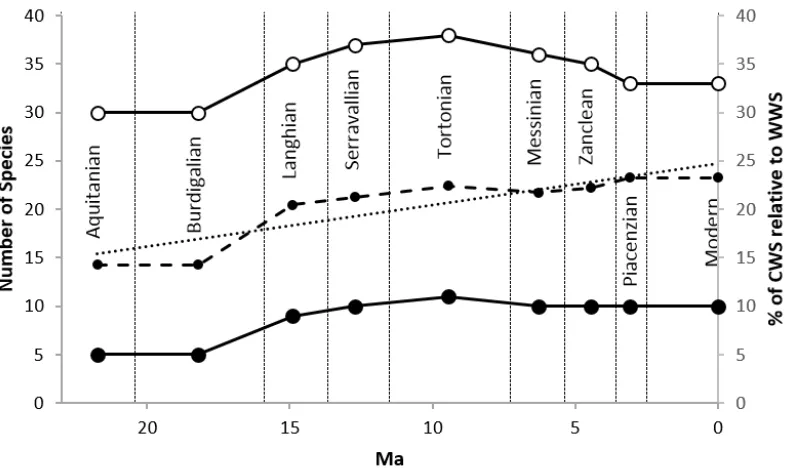
Figure 8: The number of dinoflagellate cyst species with warm or cold water preferences for each stage are plotted on 453

the left axis and the percentage of Cold Water Species (CWS) that make up the total number of species with known 454

temperature preferences for each stage (black dashed line) are plotted on the right axis. The data were obtained by 455

counting the number of species in each stage from the range chart in Figure 3. 456

Throughout the Neogene, there is a significantly higher number of WWS than CWS (Figure 8). This is 457

likely due to the latitudinal biodiversity gradient where the warmer, lower latitudes have a higher 458

diversity than the cooler, higher latitudes. This phenomenon has been observed in the geological 459

record for at least the last 30 Myr (Crame, 2001; Mittelbach et al., 2007; Mannion et al., 2014). This 460

relatively low species richness of CWS is an enduring feature of the dinoflagellate cyst record, and 461

hence does not affect our interpretations. There are fewer localities in the most northerly/southerly 462

latitudes, which potentially led to higher numbers of WWS compared to CWS in the database. 463

However, as this is consistent throughout the Neogene, it is unlikely to bias our results. 464

32

4.7

Uncertainty from geographical and temporal distribution of data

466

The majority of CWS occurrences are in the Northern Hemisphere (Figure 4). This is a clear sampling 467

bias due to the lack of Neogene dinoflagellate cyst records from the Southern Hemisphere (Figure 4). 468

For this reason, the mean percentage of CWS for each stage (Figure 6a) was recalculated only using 469

the records from the Northern Hemisphere (Figure 6b). The most obvious difference between the 470

two methods (global versus northern only) was in the Tortonian. The mean percentage of CWS was 471

higher for the Tortonian than for the immediately adjacent stages. This difference for the Tortonian 472

can be explained by the Southern Hemisphere having substantially more records than in the other 473

time intervals (Figures 4e, 5a), the majority of which have CWS values of 33% or higher. These 474

records, between 65 and 70° S and 20 to 25° S, are numerous, with tightly constrained ages, and 475

result in a much larger percentage of CWS in the Tortonian (19%, Figure 6a) than in the stages below 476

and above (5% in the Serravallian and 12% in the Messinian). When only using data from the 477

Northern Hemisphere, which has a more equal spatial distribution, there is a reduced discrepancy 478

between the Tortonian and the immediately adjacent stages (Figure 6b). It is for this reason that the 479

conclusions drawn from this study mainly concern the Northern Hemisphere. As the majority of data 480

in the Northern Hemisphere were collected from the North Atlantic and Arctic oceans and the 481

Mediterranean region, it is likely that the signal produced is from those areas, rather than for the 482

whole of the Northern Hemisphere. 483

This implies that care must also be taken in the Northern Hemisphere in latitudinal bins that are 484

devoid of data for some of the stages. For example, the three most northerly latitudinal bins only 485

have data for the Pliocene, all of which have high percentages of CWS. To ensure that the Pliocene 486

data were not skewing the results, further analysis of the data was carried out excluding latitudinal 487

bins that did not have data for all stages (Figure 6b). Comparing results using all the Northern 488

Hemisphere data, to those using simply latitudinal bins with data present for every stage (Figure 6b), 489

33 used. However, the overall trend is the same, and leads to the conclusion that the absence of data in 491

the high latitudes for stages other than the Pliocene has not skewed the results. 492

The average age range of the records for each stage is variable (Figure 9). The records from the 493

Aquitanian and Burdigalian have the longest age range (4.7 and 4.4 Myr respectively), and the 494

Zanclean and Piacenzian records have the shortest age ranges (0.9 and 0.8 Myr respectively). This is 495

partly due to the nature of the dating. For example, many of the records dated in the literature are 496

dated to within a stage or in some cases, to the nearest sub-epoch (i.e. the Early Miocene). Thus, the 497

records of the longer stages, such as the Burdigalian (spanning 4.47 Myr) have a higher average age 498

range, while the Piacenzian (the shortest stage of the Neogene; 1.02 Myr in duration) has a much 499

lower average record length. Unfortunately, this means that any evidence of short scale events 500

affecting dinoflagellate cysts, such as the MMCO and the mPWP, is not resolved in this study. 501

Further to this an individual data- of the Neogene 502

orbital cycle (Salzmann et al., 2013; Liebrand et al., 2017). If all the records used to define the %CWS 503

504

direction. Despite this uncertainty in the time-averaging approach applied to Neogene dinoflagellate 505

cyst records a trend from low %CWS during the Early Miocene to high %CWS in the Late Pliocene is 506

seen. It is therefore still possible to interpret long-term changes and, in the future, the generation of 507

higher-resolution dinoflagellate cyst records would facilitate more detailed studies of climate and 508

environmental change. 509

510

34 512

Figure 9: The average duration of dinoflagellate cyst records for each stage. Generally, temporal resolution of the data is 513

higher in shorter stages because much of the data are dated to within a stage. 514

515

5.

Discussion

516

5.1

Driving factor of the cooling Neogene

517

The increase in CWS through the Neogene (Figures 6, 7) strongly supports the cooling trend seen in 518

the benthic oxygen isotope stack, global vegetation records and global alkenone data (Zachos et al., 519

2008; Pound et al., 2012a; Salzmann et al., 2013; Utescher et al., 2015; Herbert et al., 2016). 520

Dinoflagellate cyst species that indicate cold waters are largely absent from the Aquitanian to the 521

Serravallian (Figures 6, 7). This was followed, in the Late Miocene and Pliocene, by increasing 522

proportions of CWS at individual data sites and the biogeographical expansion of cold water 523

dinoflagellate cysts species towards the lower latitudes (Figures 4, 7). By the Piacenzian, a 524

forerunner of the modern latitudinal distribution of CWS was present (Figure 7). The global scale 525

changes in dinoflagellate cysts through the Neogene points to a global scale control on Neogene 526

35 al., 2011; 2012a; Bolton and Stoll, 2013). The role of CO2 in driving Pliocene climate is well

528

established (Haywood et al., 2016), whilst it has been strongly debated whether Miocene climate 529

was also controlled by atmospheric CO2 (Knorr et al., 2011; Pound et al., 2011; Bradshaw et al., 2012; 530

Forrest et al., 2015). Much of the argument stems from older records of marine proxies for CO2, 531

which show flat-lining atmospheric CO2 or values below the pre-industrial standard of 280 ppmv for 532

most of the Miocene (Pagani et al., 1999; 2005; Beerling and Royer, 2011). The counterarguments to 533

these lines of evidence have been that these CO2 records are incorrectly calculated (Ruddiman, 534

2010) and/or the true Miocene CO2 level has yet to be detected in the record (Bolton and Stoll, 535

2013). 536

More recent records of Neogene CO2 have demonstrated higher atmospheric values and high-537

resolution fluctuations that are in tune with other climate proxy records (Zhang et al., 2013; 538

Greenop et al., 2014). Carbon dioxide as a controlling factor on Neogene climate is consistent with 539

the global scale changes in CWS dinoflagellate cysts (Figures 4, 7). Modelling results compared to 540

global datasets consistently show that higher (ca. 360-500 ppmv) CO2 levels are necessary for 541

successful simulation of Neogene climates (Dowsett et al., 2013; Bradshaw et al., 2015; Haywood et 542

al., 2016; Stap et al., 2016). The global increases in Neogene cold water dinoflagellate cysts species 543

18_{O isotope stack (Zachos et al., 2008), global changes in biome} 544

distribution through the Neogene (Pound et al., 2012a; Salzmann et al., 2013), reconstructed marine 545

and terrestrial temperatures (Utescher et al., 2015; Herbert et al., 2016), and the isotopic divergence 546

of coccolithophores (Bolton et al., 2012; Bolton and Stoll, 2013). Such diverse and widespread 547

evidence for a large-scale driver of global climate points to an overarching role of atmospheric CO2. 548

5.2

The Early Miocene (23.03 15.97 Ma)

549

Immediately prior to the Miocene, the Mi-1 event (23.13 Ma, Abels et al., 2005) in the benthic 550

oxygen isotope record shows a shift to cooler bottom waters and/or increased ice accumulation on 551

36 Liebrand et al., 2017). Recent high-resolution research has clearly demonstrated that there is much 553

more detail in the benthic oxygen isotope records than can be described using the traditional 554

Mi oxygen isotope glaciations/zones (Miller et al., 1991; Liebrand et al., 2017; Paul A. Wilson, 555

personal communication 2017). However this contribution is a global review, and we retain the Mi 556

terminology because the aim here is to compare intercontinental changes in CWS dinoflagellate 557

cysts with broad-scale perturbations in Neogene palaeoclimates. We do not propose correlations to 558

specific oxygen isotope stratigraphies. 559

Whilst evidence for ice sheets in the Northern Hemisphere is uncertain, sea-ice was present in the 560

Arctic (Larsen et al., 1994; Moran et al., 2006, DeConto et al., 2008). Ice accumulation at one or 561

potentialy both poles indicates a relatively cool climate, however, the mean CWS percentage of 2% 562

for the Aquitanian and 3% for the Burdigalian is more indicative of globally warmer oceans (Figure 563

4a, b). With the exception of occurrences off the Antarctic Peninsula, the CWS of the Aquitanian and 564

Burdigalian are not at the high latitudes and can be compared to the occurrence of CWS in the 565

modern Mediterranean Sea (Zonneveld et al., 2013b). The low numbers of CWS during the Early 566

Miocene indicates that the latitudinal temperature gradient was considerably flatter than at present 567

(Figure 7a, b). This was previously suggested by Nikolaev et al. (1998) from a compilation of 568

foraminifera and oxygen isotope data. The Early Miocene was not an interval of sustained warmth; 569

alkenone data from the Paratethys Sea shows a 2 3 °C cooling between 18.4 and 17.8 Ma (Grunert 570

et al., 2014). The Early Miocene is characterised by a 2.4 Ma eccentricity-paced benthic oxygen 571

isotope record with distinct intervals of glacial-interglacial cycles operated on a 110 ky periodicity 572

(Liebrand et al., 2017). These rapid climate and cryosphere changes are not detected in the present 573

study due to low dating resolution in many dinoflagellate cyst studies (Figure 9). 574

5.3

The Mid Miocene (15.97 11.62 Ma)

575

The Mid Miocene is both an interval of sustained global warmth (MMCO; 17-14.5 Ma) and one of 576

37 and Kennett, 1975; Zachos et al., 2001; Böhme, 2003; You et al., 2009; Quaijtaal et al., 2014). This 578

general pattern of a warm Langhian and a cooling Serravallian is recorded in the percentage of CWS 579

in each stage but higher-resolution changes in temperature are not visible due to the time slab 580

approach of the current study (Figure 6a, b T E M 18_O 581

values rapidly decreased, suggesting a reduction in continental ice and a global warming event 582

(Zachos et al., 2001; 2008). The warming event culminated in the MMCO and resulted in the tropical 583

climate zone having a much greater latitudinal extent, abundant precipitation and decreased 584

seasonality (Böhme, 2003; Bojar et al., 2004; Kroh, 2007; Pound et al., 2012a). Even though mean 585

global temperatures in the MMCO were more than 3°C higher than today (Pagani et al., 1999; 586

Kürschner et al., 2008; You et al., 2009; Foster et al., 2012), evidence for this relatively short 587

duration of warming is not obvious in this study, likely due to a lack of temporally high-resolution 588

data in the TOPIS database. 589

In addition to increased temporal resolution, improved reporting of abundance data would help to 590

identify events such as the MMCO using TOPIS. For example, Warny et al. (2009) detected the 591

MMCO in Antarctica by a 2000-fold abundance increase of just two species. These authors 592

associated the peak in productivity with increased meltwater runoff from the elevated temperatures 593

of the MMCO (Warny et al., 2009). This demonstrates how routine reporting of abundance data in 594

the literature would enhance our ability to understand Neogene climate trends. 595

What is evident from the database, is that a cooling trend occurred between the Langhian and the 596

Serravallian, which resulted in a slight increase in the percentage of CWS (Figure 6a, b). Whilst this 597

small change is apparent, it is not as characteristic as the step-like cooling demonstrated by benthic 598

18_{O values during the Serravallian (Figure 6c; Quaijtaal et al., 2014). Instead, the Serravallian} 599

consistently has higher percentages of CWS than preceding stages, indicating that dinoflagellate 600

cysts did respond to the cooling, but not uniformly in the surface waters at all latitudes. This may 601

38 first in the Southern Hemisphere during the Serravallian in response to the expansion of Antarctic ice 603

sheets (Pound et al., 2012a). Whilst the Northern Hemisphere (in the North Atlantic region at least) 604

maintained a shallower gradient, possibly in response to the onset of the warm Gulf Stream ocean 605

current (Denk et al., 2013). 606

Although 18_{O values significantly increased in the Serravallian, and less in the Tortonian,} 607

the dinoflagellate cyst record (Figure 6a-c) demonstrates the opposite. Thus, a more significant 608

cooling is indicated in the Tortonian as opposed to the Serravallian. This suggests either a time-609

averaged response of dinoflagellate cysts to the step-like cooling of the Serravallian, or that the 610

surface waters cooled at a different rate to the deep waters. Global biome reconstructions also 611

demonstrate that the cooling was more pronounced between the Serravallian and the Tortonian, 612

than the Langhian and the Serravallian (Pound et al., 2012a). This may reflect a growth of ice sheets 613

during the Serravallian, whereby 18_{O values records a combination of} 614

cooling and ice accumulation (Badger et al., 2013; Knorr and Lohmann, 2014), whereas the Late 615

Miocene did not have any additional permanent ice, but underwent continued global cooling 616

(Herbert et al., 2016). In addition, vegetation records (Pound et al., 2012a) demonstrate that the 617

Southern Hemisphere cooled prior to the Northern Hemisphere, and as the majority of the records 618

used in this study are from the Northern Hemisphere, this could be a further explanation for the 619

delayed response of the dinoflagellate cysts to the sign 18_{O values} 620

(Zachos et al., 2001; 2008). 621

During the Langhian the Central American Seaway (CAS) shoaled, potentially preventing deep water 622

exchange from around 15 Ma (Montes et al., 2015). Unfortunately there are currently no 623

dinoflagellate cyst records in TOPIS for the Caribbean during the Mid Miocene (Figure 4). However, 624

this shoaling or closure would have modified ocean circulation, and modelling results have shown 625

that this warms the Northern Hemisphere (Brierley and Federov, 2016; Lunt et al., 2008). This is 626

39 Hemisphere (Figure 4). The closure of the CAS during the Langhian would have promoted heat 628

transport into the North Atlantic. It would also have tempered the global cooling of the post-MMCO 629

climate as seen in Northern Hemisphere floras (Denk et al., 2013) and strengthened the 630

asymmetrical latitudinal temperature gradient (Pound et al., 2012a). 631

5.4

The Late Miocene (11.62 5.33 Ma)

632

The Late Miocene, though still significantly warmer than the present, was considerably cooler than 633

the Mid Miocene (Pound et al., 2012a; Utescher et al., 2015) and the Tortonian in particular (11.62 634

7.25 Ma) was characterised by warmer and more humid conditions than today (Bruch et al., 2006; 635

Pound et al., 2011). This is reflected in the increased percentage of, and wider biogeographical 636

distribution of, CWS dinoflagellate cysts (Figures 4, 5). Mean annual temperatures were between 14 637

and 16 °C in northwest Europe (Donders et al., 2009; Pound et al., 2012b; Pound and Riding, 2016). 638

Furthermore, the Cenozoic global cooling trend, which resumed at the end of the MMCO, continued 639

) H 18_{O values demonstrated that the cooling was more gradual} 640

for the Tortonian compared to the Serravallian, assuming that there was no additional ice sheet 641

growth (Figure 6c; Zachos et al., 2008). This cooling affected the presence of cold water 642

dinoflagellate cysts, and the mean percentage of CWS reached 10% in the Tortonian (Figure 6b). 643

The dinoflagellate cyst record is consistent with global vegetation records that show a cooler, more 644

seasonal, biome distribution in the Northern Hemisphere in the Tortonian, than during the 645

Serravallian (Pound et al., 2012a). Furthermore, pollen-based temperature reconstructions from 646

New Zealand demonstrate Southern Hemisphere cooling immediately after the MMCO (Prebble et 647

al., 2017). The percentage of CWS in the Tortonian in the mid to high latitudes increased, while the 648

percentage in the low latitudes remained similar to the values for the Early and Mid Miocene 649

(Figures 7a-e). The Tortonian was also the earliest stage to have all dinoflagellate cysts with known 650

temperature tolerances being CWS at 75 80° N. This indicates substantial high latitude cooling by 651

40 Arctic during the Tortonian (Stein et al., 2016). The increase in the percentage of CWS in the higher 653

latitudes compared with the low latitudes reflects that tropical regions during the Miocene remained 654

at similar temperatures, whereas the high latitudes cooled (Nikolaev et al., 1998; Williams et al., 655

2005; Steppuhn et al., 2006; Herbert et al., 2016). This effect caused the latitudinal temperature 656

gradient to steepen throughout the Late Miocene and Pliocene in the Northern Hemisphere 657

(Nikolaev et al., 1998; Crowley, 2000; Fauquette et al., 2007; Pound et al., 2012a). This temperature 658

decrease in the high latitudes was described by Nikolaev et al. (1998), who demonstrated a 4 6 °C 659

increase in the latitudinal temperature gradient between 10 and 5 Ma. Cooling of the mid to high 660

latitude surface waters during the Late Miocene is also reflected in the alkenone sea surface 661

temperature reconstructions (Herbert et al., 2016) 662

Global temperatures continued to cool through the Messinian (Pound et al., 2012a; Utescher et al., 663

2015; Herbert et al., 2016; Stein et al., 2016). However, the benthic oxygen isotope record does not 664

show a clear signal towards colder bottom water temperatures in conjunction with the evidence for 665

surface cooling (Zachos et al., 2008). Widespread alkenone data suggest that the Messinian included 666

some of the largest cooling in sea surface temperatures of the Late Miocene, and a temperature 667

minimum is recorded in the Arctic at around 6.5 Ma (Herbert et al., 2016; Stein et al., 2016). Despite 668

this, the geographical distribution and percentages of CWS dinoflagellate cysts are similar to the 669

Tortonian (Figures 4, 7). This may be an artefact of the time-slab approach, or the current available 670

data on global dinoflagellate cysts. Much of the information on Messinian dinoflagellate cysts comes 671

from the North Atlantic, which by the Late Miocene was under the influence of the Gulf Stream 672

current (Denk et al., 2013). Many of the records also lack the necessary age control and resolution to 673

identify short-lived cooling events witnessed in other records (Herbert et al., 2016; Stein et al., 674

2016). The globally distributed alkenone based sea surface temperature reconstructions suggest 675

near modern temperatures between 7 and 5.4 Ma (Herbert et al., 2016). This time interval is also 676

one of a stable climate state, with potentially higher ice volumes and a greater threshold for 677

41 consistent with Arctic surface water temperatures, dinoflagellate cysts, faunal distributions or global 679

vegetation records (Donders et al., 2009; Pound et al., 2012a; Utescher et al., 2015; Azpelicueta and 680

Cione, 2016; Stein et al., 2016; Prebble et al., 2017). 681

The presence of CWS dinoflagellate cysts in the Late Miocene of offshore South Africa (Figure 4) has 682

been used as an indicator for the presence of the cold Benguela Current (“ D 683

Haass et al., 1990; Robert et al., 2005; Heinrich et al., 2011; Hoetzel et al., 2017). The slightly 684

reduced number of cold water dinoflagellate cysts in the Mediterranean during the Messinian, when 685

compared to the Tortonian, is in agreement with alkenone data that shows warmer Messinian Sea 686

Surface Temperatures (SSTs) than in the latest Tortonian (Tzarnova et al., 2015). The temporal 687

resolution of the dataset does not allow any response to the Messinian Salinity Crisis to be detected 688

(Flecker et al., 2015), especially since the global-scale climate effects would have been limited in 689

magnitude and extent, and transient (Ivanovic et al., 2014). 690

5.5

The Pliocene (5.33 2.58 Ma)

691

In the Pliocene, the trends towards cooler climates continued and was interrupted by brief warm 692

intervals (Haywood et al., 2013; 2016; Salzmann et al., 2013). Despite being cooler than the 693

Miocene, the Pliocene was still significantly warmer than today (Haywood et al., 2013; Salzmann et 694

al., 2013; Pound et al., 2015; Dowsett et al., 2016; Panitz et al., 2016) with a shallower Northern 695

Hemisphere latitudinal gradient of CWS-dominated dinoflagellate cyst assemblages compared to the 696

modern (Figure 7). The percentage of CWS increased most markedly in the high latitudes, from 45° N 697

northwards (Figure 7e, f), thereby further steepening the latitudinal temperature gradient. Nikolaev 698

et al. (1998) found that the latitudinal gradient increased by 4 5 °C during the Piacenzian, and 699

Fedorov et al. (2013) demonstrated a 4 7 °C cooling of the mid to high latitudes of the North 700

Atlantic and Pacific oceans. This cooling of the higher latitudes compared to the lower latitudes is a 701

42 Pound et al., 2012a; Federov et al., 2013; Herbert et al., 2016), and was associated with the

703

development of ice in the high latitudes (Dolan et al., 2011; Dowsett et al., 2016). 704

Short-lived glaciations were infrequent in the Zanclean, but became more common in the Piacenzian 705

as the global climate continued to cool (Lisiecki and Raymo, 2005; Miller et al., 2005; 2012). A 706

generally warmer Zanclean, and a cooler Piacenzian, is consistent with the average percentage of 707

CWS dinoflagellate cysts in the Zanclean (16%) and the Piacenzian (23%; Figure 4), and is consistent 708

with global alkenone records (Herbert et al., 2016). However, short-lived glaciations are not 709

currently detectable in the TOPIS database due to the limitations of sampling resolution. The East 710

and West Antarctic ice sheets were both well established by this time (Naish and Wilson, 2009; 711

Dolan et al., 2011). Although the Southern Hemisphere lacks widespread dinoflagellate cyst records 712

for the Piacenzian, the two data points proximal to the Antarctic Peninsula contain 100% CWS 713

dinoflagellate cysts (Figure 4). Ice sheets in the Northern Hemisphere were significantly smaller, 714

compared to the modern, or absent, which is consistent with WWS dinoflagellate cysts still being 715

present in the high latitudes of the North Atlantic (Figure 4; Dolan et al., 2011; De Schepper et al., 716

2014; Panitz et al., 2016). Global climate started to significantly deteriorate (cooled) in the 717

Piacenzian, leading to the intensification of the Northern Hemisphere glaciation around 2.75 Ma 718

(Ravelo et al., 2004; Mudelsee and Raymo, 2005; De Schepper et al., 2014; Panitz et al., 2016). 719

The CAS continued to constrict during the Pliocene before finally closing around the Pliocene 720

Pleistocene boundary (Coates and Stallard, 2013; Osbourne et al., 2014). Neodymium isotopes show 721

the exchange of waters until 2.5 Ma, but deep water exchanges had ceased by 7 Ma (Coates and 722

“ O I M C 18_{O suggest}

723

that this continued constriction lead to greater heat transport in the Zanclean into the Northern 724

Hemisphere, but reduced heat transport during the Piacenzian (Bailey et al., 2013; Karas et al., 725

2017). These results are consistent with the latitudinal distribution of CWS dinoflagellate cysts in the 726