From Line Drawings to Human Actions: Deep Neural Networks for Visual Data Representation

(1)

From Line Drawings to Human

Actions: Deep Neural Networks for

Visual Data Representation

Fang Wang

A thesis submitted for the degree of

Doctor of Philosophy of

The Australian National University

(2)

(3)

Declaration

Except where otherwise indicated, this thesis is my own original work.

Fang Wang 7 November 2017

(4)

(5)

Acknowledgments

I would like to express my deepest gratitude to my supervisors Dr. Yi Li and Prof. Fatih Porikli. They provided me great supports and encouraged me to continue my research when things became hard. Their passions about research and vision of the future directions in computer vision inspired me deeply. It has been my great pleasure to work with them in the past few years. I am grateful for their patient supervision on research, careful guidance on shaping immature ideas, and late night editing on papers. Furthermore, I would like to thank Dr. Justin Domke for providing valuable suggestions along the journey towards my Ph.D. degree.

Further, I would like to express my sincere appreciation to Prof. Cornelia Fer-müller and Prof. Yiannis Aloimonos. They gave me great support and invaluable advice during my visiting in the Computer Vision Laboratory at the University of Maryland. They have always been supportive and kind to me in the past few years. I have been fascinated by their pioneering ideas of the research in computer vision and robotics. I was very fortunate to have the opportunity to work with them. Their insightful discussions about the research area kept me motivated during my study.

I would like to thank Le Kang, Aiwen Jiang, Yezhou Yang, Konstantinos Zam-pogiannis, Yi Zhang, Francisco Barranco, Michael Pfeiffer, and Chinmaya Devaraj, who have collaborated with me and contributed amazing efforts in our studies. They showed me how to effectively shape research ideas and execute pioneer research. I thank my colleagues and friends at the Australian National University, who gave me valuable support and help during my study. My thanks go to Hanxi Li, Lin Gu, Tianxing Li, Dylan Campbell, Buyu Liu, Wei Zhuo, Haoyang Zhang, and Gao Zhu. I would also like to thank my friends at the University of Maryland, Ren Mao, Tao Wen, Fangyi Zhang, Kanishka Ganguly, Gregory Kramida, and Aleksandrs Ecins. Thank you for giving me so much wonderful time during my visiting and I have learned a lot from you all.

Finally, I would like to show my deepest thanks to my family. Thank you for your love and trust. You have encouraged me all the time and always been my strongest backing. Without you, I could never be where I am today.

(6)

(7)

Abstract

In recent years, deep neural networks have been very successful in computer vi-sion, speech recognition, and artificial intelligent systems. The rapid growth of data and fast increasing computational tools provide solid foundations for the applica-tions which rely on the learning of large scale deep neural networks with millions of parameters. The deep learning approaches have been proved to be able to learn powerful representations of the inputs in various tasks, such as image classification, object recognition, and scene understanding. This thesis demonstrates the generality and capacity of deep learning approaches through a series of case studies includ-ing image matchinclud-ing and human activity understandinclud-ing. In these studies, I explore the combinations of the neural network models with existing machine learning tech-niques and extend the deep learning approach for each task. Four related tasks are investigated: 1) image matching through similarity learning; 2) human action pre-diction; 3) finger force estimation in manipulation actions; and 4) bimodal learning for human action understanding.

Deep neural networks have been shown to be very efficient in supervised learn-ing. Further, in some tasks, one would like to group the features of the samples in the same category close to each other, in additional to the discriminative repre-sentation. Such kind of properties is desired in a number of applications, such as semantic retrieval, image quality measurement, and social network analysis, etc. My first study is to develop a similarity learning method based on deep neural networks for image matching between sketch images and 3D models. In this task, I propose to use Siamese network to learn similarities of sketches and develop a novel method for sketch based 3D shape retrieval. The proposed method can successfully learn the representations of sketch images as well as the similarities, then the 3D shape retrieval problem can be solved with off-the-shelf nearest neighbor methods.

After studying the representation learning methods for static inputs, my focus turns to learning the representations of sequential data. To be specific, I focus on manipulation actions, because they are widely used in the daily life and play impor-tant parts in the human-robot collaboration system. Deep neural networks have been shown to be powerful to represent short video clips [Donahue et al., 2015]. However, most existing methods consider the action recognition problem as a classification

(8)

task. These methods assume the inputs are pre-segmented videos and the outputs are category labels. In the scenarios such as the human-robot collaboration system, the ability to predict the ongoing human actions at an early stage is highly impor-tant. I first attempt to address this issue with a fast manipulation action prediction method. Then I build the action prediction model based on Long Short-Term Mem-ory (LSTM) architecture. The proposed approach processes the sequential inputs as continuous signals and keeps updating the prediction of the intended action based on the learned action representations.

Further, I study the relationships between visual inputs and the physical infor-mation, such as finger forces, that involved in the manipulation actions. This is motivated by recent studies in cognitive science which show that the subject’s inten-tion is strongly related to the hand movements during an acinten-tion execuinten-tion. Human observers can interpret other’s actions in terms of movements and forces, which can be used to repeat the observed actions. If a robot system has the ability to estimate the force feedbacks, it can learn how to manipulate an object by watching human demonstrations. In this work, the finger forces are estimated by only watching the movement of hands. A modified LSTM model is used to regress the finger forces from video frames. To facilitate this study, a specially designed sensor glove has been used to collect data of finger forces, and a new dataset has been collected to provide synchronized streams of videos and finger forces.

(9)

List of Figures

1.1 An illustration of the artificial neural network structure and the

acti-vation function. . . 2

2.1 A typical convolutional neural network structure. . . 12

2.2 An Recurrent Neural Network and the unfolded structure. . . 13

2.3 A diagram of a LSTM memory cell. . . 14

2.4 A typical Siamese network structure. . . 17

3.1 Examples of sketch based 3D shape retrieval. . . 22

3.2 An illustrated example of cross-domain similarity learning. . . 26

3.3 Dimension reduction using Siamese network. . . 27

3.4 3D models viewed from predefined viewpoints. . . 29

3.5 Line rendering of a 3D model. . . 29

3.6 Retrieval examples of PSB/SBSR dataset. . . 32

3.7 Retrieval examples of unseen samples in PSB/SBSR dataset. . . 34

3.8 Split test set performance on SBSR. . . 34

3.9 Visualization of feature space on SHREC’13. . . 35

3.10 Performance comparison on SHREC’13. . . 36

3.11 Performance comparison on SHREC’14. . . 37

3.12 Sketch-sketch retrieval on SHREC’13. . . 38

3.13 View-view retrieval on SHREC’13. . . 39

4.1 Two examples demonstrate that early movements are strong indicators of the intended manipulation actions. . . 42

4.2 The flowchart of the action prediction model, where the LSTM model is unfolded over time. . . 49

4.3 Interface used in the human study. . . 51

4.4 Human prediction performance. . . 52

4.5 Prediction accuracies over time for the five different objects. . . 54

(14)

4.7 Confusion matrix of action classification. . . 57

4.8 Samples of action prediction on the 50 Salad dataset. . . 59

4.9 Comparison of prediction accuracies between our computational method and data from human observers. . . 60

5.1 Illustration of the hand force estimation. . . 63

5.2 The flowchart of the force estimation model. . . 65

5.3 Illustration of the force-sensing device. . . 67

5.4 Force data collection and preprocessing. . . 68

5.5 Samples of force estimation results. . . 71

6.1 The network structure of the hallucination network. . . 78

6.2 Sample actions of the 50 salads dataset. . . 82

(15)

List of Tables

3.1 Precision-recall on fixed points. . . 33

3.2 Standard metrics on the PSB/SBSR dataset. . . 33

3.3 Comparison on SHREC’13 dataset. . . 37

3.4 Comparison on SHREC’14 dataset. . . 38

3.5 Standard metrics for the within-domain retrieval on SHREC’13. . . 39

4.1 Object and Action pairs of MAD . . . 50

4.2 Comparison of classification accuracies on different objects . . . 56

4.3 Comparison of classification accuracies on the 50 Salad dataset. . . 59

5.1 Object and Action pairs of HAF . . . 69

5.2 Average errors of estimated force for each finger (unit in N). . . 70

5.3 Average errors of estimated force for each action (unit in N). . . 70

5.4 Action prediction accuracy. . . 72

6.1 Results for the 50 SALADS dataset. . . 83

6.2 Results for the HAF dataset. . . 84

(16)

(17)

Chapter1

Introduction

In the last five years, we witness the rapid development and significant success of deep learning methods in both academia and industry. The idea of automatically learning of features has been shown to be more efficient than the traditional feature engineering methods with domain knowledge. Some notable applications include image classification and natural language processing. It may be interesting to raise the question about what applications, in additional to these mainstream ones, can benefit from deep learning. This thesis is an attempt to answer this question with deep analysis and case studies of applications. The studies in this thesis focus on the deep learning methods and their variations to solve computer vision tasks that traditionally have been considered difficult. The research work in this thesis is two folded. One is the learning of static inputs such as images. The other one is the learning of dynamic inputs with temporal information such as videos.

The performance of existing computer vision algorithms depends heavily on the representations or features of the given inputs. Traditional learning algorithms rely on manually designed features for specific data in different tasks, such as human speech, language, handwritten texts, and natural images. This procedure is called feature engineering, which requires expert knowledge of the given inputs as well as a certain understanding of the learning algorithms to design a good feature. Such procedures are very inefficient because they usually do not generalize well across do-mains. Based on these handcrafted features, researchers have proposed many learn-ing algorithms that are proved to be successful for computer vision, for example, naive Bayes [Russell and Norvig, 2003], logistic regression [Cox, 1958] and support vector machines [Cortes and Vapnik, 1995], etc. However, most of these methods treat the features as fixed inputs or perform simple preprocessings to the input fea-tures. One step towards the feature learning is the sparse coding method, which aims at finding the representation of input data by learning the linear combination of a

(18)

[image:18.595.83.473.139.289.2]

(a) (b)

Figure 1.1: An illustration of the artificial neural network structure and the activation function. (a) In an artificial neural network, a number of hidden layers with neural units are used to connect the input and the output layers. (b) The activation function takes the weighted summation of the inputs and generates the output response with a non-linear function.

set of basic feature elements [Olshausen and Field, 1996; Donoho and Elad, 2003]. In this way, the model can learn a sparse representation for each input. However, the basic elements are still manually defined and the model can only learn simple combinations of the basis with a shallow structure.

(19)

§1.1 Deep neural networks 3

To represent highly complex and redundant inputs such as natural images, a large scale artificial neural network with millions of units is necessary. However, training of such large scale networks requires plenty of computational resources and labeled training samples, which limits their usage.

In recent years, the rapid accumulating of data makes it possible to collect large scale datasets with millions of training samples. Further, the emergence of fast paral-lel computing devices enables the development of learning algorithms that have high computational cost. Both these new developments make the training of large scale neural network possible. These large scale neural networks are called deep neural networks since they usually consist of many connected neural layers and form a deep structure. The deep neural networks are derived from the traditional artificial neu-ral networks. Different from the other popular machine learning methods that have shallow structures, deep neural networks typically have more layers and parame-ters, thus they have the potential to represent more complex inputs. These complex networks allow people to build intelligent agents that are capable of complicated perception tasks and even reach the performance of human in some cases.

In the following sections of this chapter, Section 1.1 introduces the basic concepts and commonly used tools in deep learning, and discusses the typical neural network structures for different tasks. Section 1.2 discusses the deep learning approaches for static input learning. It briefly introduces the popular network structures used for discriminative learning as well as similarity learning tasks. Section 1.3 discusses about deep learning methods for sequential data. This section introduces the net-work structures that can handle sequential inputs. These netnet-works have temporal recursive loops and are suitable for modeling the dynamics in sequential data. In this thesis, I use these network architectures to learn representations of human ac-tions and briefly introduce three related tasks about manipulation action recognition. At last, the outline of the whole thesis is given in Section 1.4 and a list of publications is presented in Section 1.5.

1 .

1 Deep neural networks

(20)

non-linear relationships. The hidden units are connected with all or partial of the units in the previous layer and feed the outputs forward to the next layer. With the stacked structure of many hidden layers, the deep neural network is able to learn multiple levels of feature representations that correspond to different levels of abstraction. Analysis of the weights in each layer shows that the earlier layers can extract the lower level patterns from the inputs, and the latter layers tend to learn high-level features by combining the lower level patterns [Zeiler and Fergus, 2014]. With such structures, the deep neural networks are able to extract complex representations.

A deep neural network can be trained using standard backpropagation method. Rumelhart et al. [1988] showed that it is possible to train the hidden units in a neural network to represent the important features of the task domain using backpropaga-tion method. For each training input, the backpropagabackpropaga-tion algorithm first calculates the response of each unit in the network using the forward procedure. Next, the out-puts are compared with the ground-truth labels to calculate the error or loss. Then this error can be propagated back to all units and get the adjust value of the unit pa-rameters. The standard backpropagation method for training deep neural networks is the stochastic gradient descent (SGD) method. It converges much faster than the batch gradient descent method. In practice, an alternation of the stochastic gradient descent method is often used which is call “mini-batch” gradient descent. Other than calculating the gradient updates for each training sample, the “mini-batch” method uses multiple training samples at each step. This is a good compromise between the standard batch gradient descent and the global gradient descent method. One benefit is that with multiple training samples at each step, one can utilize the paral-lel computing tools to accelerate the training process. Another benefit is that using “mini-batch” makes the training process more stable than using individual inputs because it uses multiple training samples for gradient updates in each step.

1 .

2 Learning of static inputs

(21)

§1.3 Learning of sequential data 5

processing grid-like data such as speech signals (1D grid) and images (2D grids). To automatically learn features from image inputs, an important ability is to be robust to deformations and image noise. CNN models use max-pooling layers to learn robust features and handle deformations. With these techniques, the CNNs have shown to be effective in both vision and speech tasks. For example, in the ImageNet Large Scale Visual Recognition Competition (ILSVRC) [Russakovsky et al., 2015], over one million images are used to train a 1000-way classifier. In this scenario, convolution neural networks achieved the best performance on both classification and detection tasks, and the best method reported less than 3% classification errors over 1000 categories [ILSVRC, 2016], which is competitive with the performance of human recognition.

Although the CNN model is able to learn powerful representations for discrim-inative learning, in some tasks we would like to learn the representation that more similar objects have smaller distances. Such kind of properties is desired in a number of applications, for example, semantic retrieval, image quality measurement, and so-cial network analysis. In computer vision, the Siamese network has been adopted for face verification [Chopra et al., 2005] and digit recognition [Yih et al., 2011]. It uses a shared deep neural network to learn features from pairs of samples instead of pro-cess individual samples. Then the extracted features are compared with a contrastive loss function, which allows the Siamese network to learn the feature representations as well as the similarities for pairs of data.

In this work, the Siamese network is studied and applied to solve the sketch based 3D shape retrieval problem. Existing methods for 3D shape retrieval depend on handcrafted features and extensive searching for the best viewpoint to match the 3D models and the 2D sketches. The proposed method using learned shape representations for shape matching, which is shown to be superior to traditional shape features. We show that the learned features using deep neural networks are good for cross-domain similarity learning as well as simple sketch matching.

1 .

3 Learning of sequential data

(22)

etc. To model sequential data, the Recurrent Neural Network (RNN) is the most frequently used network architecture. RNN contains a recursive loop that unfolds over time, which makes it suitable for modeling non-linear time series with long time correlations. RNN has been widely used in natural languages processing as well as video sequences modeling. However, the traditional RNN is hard to train using gradient descent method because of the vanishing gradient problem. To tackle this problem, the Long Short-Term Memory (LSTM) model is then proposed. It introduces memory cells with gates control, which makes the LSTM architecture more robust when learning temporal dynamics with long time constants.

This thesis focuses on the human action recognition problem to explore the rep-resentation learning method of sequential data. Human action recognition is one of the fundamental problems in computer vision. Due to its high complexity, many research works try to simplify the visual inputs into a set of key points and only focus on the trajectories of these key points to model the dynamics [Laptev, 2005; Rohrbach et al., 2012; Wang et al., 2011]. Other researchers aim at finding spatial-temporal representations that are suitable for action recognition [Dollár et al., 2005; Laptev and Lindeberg, 2006; Klaser et al., 2008; Scovanner et al., 2007]. With all these efforts, it is still challenging to learn a good representation of human actions and model the dynamics. In this thesis, I study the effectiveness of the recurrent neural network architecture in human action recognition. The goal is to understand how to effectively learn a good representation of human actions using neural networks. To be specific, three aspects of the action recognition problem has been investigated. 1) I propose to predict the intended actions as a continuous task instead of classifying the actions for segmented video clips. 2) I propose to estimate the physical motoric information such as finger forces by watching the hand movements. 3) I explore the bimodal learning for action recognition to utilize the physical information to improve the recognition performance.

1.3.1 Predicting actions

(23)

§1.3 Learning of sequential data 7

In this thesis, I focus on hand manipulation actions that are often involved in human-robot collaboration tasks. For a robotic system, it is essential to have the ability to update the beliefs about the observed actions and predict the intended actions of their human counterpart. An efficient action prediction method needs well-learned action representations that are able to discriminate the subtle differences of the early hand movements. Therefore, I proposed to build an action prediction model based on the LSTM architecture. The proposed approach processes the sequential inputs as continuous signals and generates confidence map over all candidate action categories for each frame. With the recurrent loops in the LSTM architecture, the history information is implicitly encoded in the model, so that the prediction for each frame is based on both the latest input as well as the previous visual inputs. In this way, the prediction model is able to update the confidence of action categories along with time changes.

This is a challenging task since we are aiming at distinguishing the intended action by watching the dexterous movements of hands. The convolutional neural networks are known to represent image frames, and the recurrent neural networks are designed to learn the dynamic changes of sequential inputs. So we combined these two models in our proposed method to make use the representative power of both these architectures. With this combination, our method is able to capture the delicate differences of the dynamics of the manipulation actions.

1.3.2 Predicting hand forces

Recent studies in cognitive science show that the subject’s intention is strongly re-lated to his/her movements during an action execution. Also, the physical contacts between hands and the objects can be altered with different attentions. For exam-ple, when a subject intends to use a hammer to pound a nail, it is highly likely that he/she will grasp with more forces than just to passing the tool. Human observers can easily interpret other’s actions in terms of movements and forces, and predict the consequences driven by these patterns. If a robot system can estimate the force patterns from videos, it will be able to learn how to manipulate an object by watching video demonstrations.

(24)

frames. To train this model, videos of manipulation actions need to be collected with synchronized streams of force measurements on the hand. This was done with a specially designed sensor glove that attached force sensors to the fingertips.

1.3.3 Learning with bimodal information

With the action prediction model and the hand forces regressor, it is natural to ask how to combine the additional information with vision inputs to improve action pre-diction performance. In many real applications, the additional information, such as accelerometer data, hand forces, gazing points, needs to be gathered with special de-vices. This limits the use of bimodal learning approaches. To alleviate this problem, I explore a bimodal learning method that can learn the relationship between the two input streams and use the learned representation to improve manipulation action recognition for samples that do not have the additional information.

Motivated by the success of the hand force regression model, a natural idea is to make use of the hand forces to help with the action recognition. One simple exten-sion is to directly use the regresexten-sion model and generate estimations of hand forces and train the recognition model on both vision input and the forces. However, such framework fails to model the relationship between the hand forces and the vision inputs, which is crucially important for a bimodal learning model. To model the relationship between videos and forces, a possible solution is to learn a hallucination network to bridge the two inputs. During the training stage, the hallucination net-work dedicates to approximate the learned representation of the forces using vision inputs, so that it can learn the relationship between video frames and hand forces. During the testing stage, the hallucination network can generate a simulated repre-sentation of the forces. The whole network is trained end-to-end to jointly learn the action recognition model as well as the hallucination network.

1 .

4 Thesis outline

The remain of this thesis is organized as follows:

(25)

§1.5 Publications 9

Chapter3: Sketch Based3D Shape Retrieval This chapter describes a case study of representation learning for sketches to solve the problem of sketch based 3D shape retrieval. A similarity learning method for matching sketch images using Siamese network is proposed. This work was published in CVPR 2015.

Chapter 4: Manipulation Action Prediction Using LSTM To study the represen-tation learning methods of sequential data, we focus on human manipulation action recognition tasks. In this chapter, I show how to use the RNN and LSTM models to learn representations of manipulation actions and proposed a novel approach to predict intended actions while watching the manipulation movements. This work was published in IJCV, Special Issue on Chalearn: Looking at people, 2017.

Chapter5: Hand Force Prediction Using LSTM This chapter demonstrates how to estimate hand forces from vision input. The LSTM model is adopted for regression of the hand force. I show that the estimated forces can be used to improve the action recognition performance. A new dataset is collected with synchronized sequences of hand forces and action videos to evaluate the proposed method.

Chapter6: Manipulation Action Recognition Using Bimodal Inputs This chapter expands the manipulation action recognition method to incorporate with additional information such as hand forces or motoric data of the tools or objects that involved in the actions. I show how to train a hallucination network for sequential inputs, and generate hallucinated representations of the additional information for action recognition tasks. This work was submitted to ICCV, 2017.

Chapter7: Conclusion Finally, we summarize the main contributions in this thesis and discuss the future directions.

1 .

5 Publications

During my study in NICTA/ANU, I have published the following papers:

Journal publications:

(26)

2. Cornelia Fermüller, Fang Wang, Yezhou Yang, Konstantinos Zampogiannis, Yi Zhang, Francisco Barranco, and Michael Pfeiffer. "Prediction of Manipulation Actions." IJCV, Special Issue on Chalearn: Looking at people, 2017.

Conference publications:

1. Chinmaya Devaraj, Fang Wang, Yi Li, Cornelia Fermüller, and Yiannis Aloi-monos. "Leveraging Motoric Information for Recognizing Manipulation Ac-tions" (Submitted to ICCV 2017)

2. Fang Wang, Le Kang, and Yi Li. "Sketch-based 3d shape retrieval using convo-lutional neural networks." CVPR 2015.

3. Fang Wang and Yi Li. "Spatial matching of sketches without point correspon-dence." ICIP 2015.

4. Fang Wang and Yi Li. "Beyond physical connections: Tree models in human pose estimation." CVPR 2013.

(27)

Chapter2

Background and Related Work

In recent years, deep learning has achieved great success in speech processing and computer vision tasks. Unlike the traditional methods that try to manually design features for specific inputs, deep learning provides a powerful tool to learn represen-tations directly from inputs. The idea of learning features automatically from inputs is attractive because it relieves the need of expert knowledge to extract useful fea-tures for specific tasks. Recent studies show that the data driven feature engineering methods often have better performance than handcrafted features. This is possibly because the automatically learned features can capture more discriminative features. In this chapter, we introduce the basic concepts of deep learning approaches and briefly discuss the key techniques that are used for training of deep neural networks. Section 2.1 revisits the basic concepts of deep neural networks and introduces a fre-quently used network structure in representation learning approaches. In Section 2.2, several special network structures are introduced as the backgrounds of our case studies. Section 2.2.1 introduces the Siamese network for matching problem. Sec-tion 2.2.2 introduces the recent models for sequential data learning.

2 .

1 Deep neural network structures

Deep neural networks are a series of neural network structures that consist of many neural layers. With a deep structure, a neural network can effectively learn compli-cated mappings from the inputs to the target using end-to-end training, which does not rely on domain knowledge. Several techniques have been devised to overcome the difficulties in the training of complex neural networks.

(28)

2.1.1 Convolution neural network

A convolutional neural network (CNN) is a neural network that is suitable for pro-cessing images. As indicated by its name, the core component in CNN is the con-volutional layer, which applies the "convolution" operation on the layer inputs to filter out useful information. The second important component is the pooling layer, which downsamples the inputs using a given selection method. The last is the fully connected layer, which combines all the outputs of the previous layer and gener-ates the feature representations. With a deep structure, a CNN can effectively learn complicated mappings from raw images to the target, which requires less domain knowledge compared to handcrafted features and shallow learning frameworks.

[image:28.595.74.488.437.532.2]

A typical CNN structure consists of several convolutional layers that have a small field of perception, and a few fully connected layers that each combines all the out-puts from the last layer and yields a feature vector with several thousands of dimen-sions. To efficiently train the CNN model, the standard method is using Stochastic Gradient descent (SGD) with backpropagation algorithm. Figure 2.1 shows the struc-ture of AlexNet, which is one of the early CNN models.

Figure 2.1: A typical convolutional neural network structure (Redraw of the AlexNet structure [Krizhevsky et al., 2012]).

(29)

§2.1 Deep neural network structures 13

comprehensive representations through millions of training samples, the finetuning procedure can start from exploring useful representations for the new task without going all the way from scratch.

2.1.2 Recurrent Neural Network

[image:29.595.166.472.361.480.2]

The Recurrent Neural Network (RNN) is a popular architecture that has been widely used to processing sequential inputs, such as natural language and video frames. The RNN model has a temporal recurrent loop that can capture compositional repre-sentations in the time domain and is suitable for modeling the dynamic of sequential inputs. The temporal recurrent loop creates a deep structure in the RNN model when unfolding in the time series. Figure 2.2 shows the structure of RNN and the unfolded network.

Figure 2.2: An Recurrent Neural Network and the unfolded structure.

Given a sequence x = {x1,x2, . . . ,xT}, an RNN computes a sequence of hidden statesh=_{h1,h2, . . . ,hT}and outputsy ={y1,y2, . . . ,yT}as follows:

ht=H(Wihxt+Whhht 1+bh) (2.1)

yt=O(Whoht+bo), (2.2)

where Wih,Whh,Who denote weight matrices, bh,bo denote the biases, andH(·)and O(_·)are the activation functions of the hidden layer and the output layer, respectively. Typically, the activation functions are defined as logistic sigmoid functions.

(30)

[image:30.595.135.415.108.272.2]

Figure 2.3: A diagram of a LSTM memory cell (adapted from Graves et al. [2013]).

of backpropagation steps, which makes the training extremely slow. This problem limits the maximum length of sequences that an RNN can accept.

To alleviate the vanishing gradient problem, the Long Short-Term Memory (LSTM) model is then proposed by Hochreiter and Schmidhuber [1997]. Specifically, in ad-dition to the hidden state ht, the LSTM also includes an input gate it, a forget gate

ft, an output gateot, and the memory cell ct (shown in Figure 2.3). These gates are regularized with sigmoid functions and control the portion of information passed through the update functions. To be specific, in this architecture it and ft are sig-moidal gating functions, and these two terms learn to control the portions of the current input and the previous memory that the LSTM takes into consideration for overwriting the previous state. Meanwhile, the output gate ot controls how much of the memory should be transferred to the hidden state. These mechanisms allow LSTM networks to learn temporal dynamics with long time constants.

The hidden layer and the additional gates and cells are updated as follows:

it =s(Wxixt+Whiht 1+Wcict 1+bi) (2.3)

ft =s(Wx fxt+Wh fht 1+Wc fct 1+bf) (2.4)

ct= ftct 1+ittanh(Wxcxt+Whcht 1+bc) (2.5)

ot =s(Wxoxt+Whoht 1+Wcoct+bo) (2.6)

ht =ottanh(ct) (2.7)

(31)

§2.1 Deep neural network structures 15

[Visin et al., 2014], and the estimation of object motion [Fragkiadaki et al., 2015]. Ng et al. [2015] used the LSTM model to learn dynamic changes for action recognition.

Although the LSTM is the most commonly used structure, other variations have been proposed to improve the performance. Cho et al. [2014] proposed a simplified version of LSTM with fewer gate controls, named Gated Recurrent Unit (GRU). It coupled the input and the forget gates into an update gate and replaced the output gate with a reset gate that only controls the recurrent connections to the block input. To improve the capability of long-term memory learning, Weston et al. [2014] pro-posed the memory networks. It introduced a long-term memory component which can learn flexible combinations of history information. This architecture provides a mechanism for selective learning of long sequences.

2.1.3 Training neural networks

(32)

Many machine-learning algorithms use variants of the standard gradient descent method for optimization. However, for the training of deep neural networks, the global gradient descent method is inefficient since calculating the sum-gradient of a large training set is extremely expensive. Many research works have been dedicated to creating efficient training methods for deep neural networks. One of the most frequently used optimization methods to train deep neural networks is the Stochas-tic gradient descent (SGD) method [Murata, 1998; Bousquet and Bottou, 2008]. This is a random optimization method that approximate the global gradient descent op-timization by accumulating gradient updates over individual samples. In practice, the gradient updates are often calculated over a small number of samples, which is also called a “mini-batch”, to utilize the parallel computational mechanisms. It also makes the convergence more smooth by using more training samples at each step. Research works show that the stochastic gradient descent converges faster than global gradient descent method. When the training set has a large number of samples, using global gradient descent is practically impossible. In such cases, the stochastic gradient descent is the best choice for the optimization.

(33)

§2.2 Applications: case studies of deep learning 17

2 .

2 Applications: case studies of deep learning

In this thesis, I use deep learning approaches for two categories of computer vision tasks: 1) similarity learning of static inputs; 2) the representation learning of sequen-tial data. This section briefly discusses the backgrounds and closely related works of the deep learning applications in the case studies.

2.2.1 Learning similarity

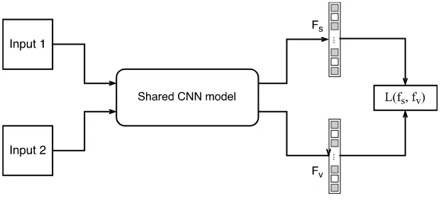
[image:33.595.163.474.516.658.2]

In this thesis, I select Siamese network as the similarity learning tool and use it to solve the sketch based 3D shape retrieval problem. A typical Siamese network structure is shown in Figure 2.4. The Siamese network has been initially proposed for signature verification [Bromley et al., 1993]. It is designed to learn the relationship of an input pair. The Siamese network consists of a shared sub-network that learn the representations of sample pairs. In different variations of the Siamese network, the shared sub-networks may be used with various network layers at different levels, then the extracted pair of features is joined at the last layers with a contrastive loss function. Different from the other single modal network structures, it learns the representation of inputs with constraints of the pairwise relationship of samples. The goal of the network is to minimize the feature distance if the input pair is labeled as similar, and push the features far away from each other for dissimilar pairs. Such kind of network structure can be used as supervised metric learning model.

Figure 2.4: A typical Siamese network structure.

(34)

achieve robustness to geometric distortions. Salakhutdinov and Hinton [2007] use multilayer neural networks with Siamese network architecture to learn non-linear embedding of high dimensional inputs. Recently, the Siamese network has been suc-cessfully applied to semantic text similarity measurements [Yih et al., 2011]. The authors show that Siamese network achieves high accuracy on cross-lingual docu-ment retrieval as well as ad relevance measure tasks, which demonstrate the ability of Siamese network to learn cross domain similarities. Chen and Salman [2011] ap-plied Siamese network for speech feature classification task and successfully learn the speaker-specific information. In recent year, the Siamese network has been adopted in more vision tasks for image matching. Zagoruyko and Komodakis [2015] extended and generalized the Siamese network to learning similarity between image patches. Bertinetto et al. [2016] further extended the Siamese network with fully convolutional networks for object tracking. Follow the line of multi-stream structures, Wang et al. [2014] proposed the triplet network for image rank learning to learn fine-grained image similarity.

2.2.2 Learning representations of sequential data

This section focuses on the deep learning approaches for sequential data modeling. Recently the RNN and the LSTM architectures have been widely used for sequen-tial data learning. They are popularized in language processing and have been used for generating sentences that describe images [Karpathy and Fei-Fei, 2015; Vinyals et al., 2015]. In these works, the recurrent networks are adopted to process the lan-guage data to either learn the lanlan-guage model or generate sentences using visual features. Instead of using recurrent networks for feature encoding, Vinyals et al. [2015] proposed to use the convolutional neural network to encode the image feature and decode it with an LSTM model. Karpathy and Fei-Fei [2015] further extended the decoding module with a bidirectional recurrent network and an attention model to generate sentences.

(35)

§2.3 Summary 19

et al., 2015] extended the LSTM model with temporal pooling over frame features and ordered sequence of frames to learn action representations.

In my study, specifically, I explore the representation learning approaches for human action recognition problem. Most traditional methods consider the action recognition problem as a classification task. Given a pre-segmented input video, the action recognition methods extract features of the video clips and generate a set of category labels as the output. In a very recent work, Ma et al. [2016] trained an LSTM using novel ranking losses for early activity detection.

2 .

3 Summary

(36)

(37)

Chapter3

Sketch Based 3D Shape Retrieval

In this chapter, my study is to learn sketch representations and similarities for shape matching. The 3D shape retrieval is an important research topic in content based object retrieval. It has important applications in computer graphics, information retrieval, and computer vision [Eitz et al., 2012b; Furuya and Ohbuchi, 2013; Li et al., 2014a]. Early studies of 3D shape retrieval directly use 3D shapes as queries and focus on creating proper feature descriptions that are suitable for 3D shape matching [Shilane et al., 2004]. Such methods suffer from the difficulty of 3D shape orientation alignment and high computational cost. Using 3D shapes as queries also limited the application of these methods. In contrast, a more intuitive approach is retrieving 3D shapes using hand drawn sketches. The idea of sketch based 3D shape retrieval is very attractive. It provides a user friendly way to create query inputs and visually depictive to specify shape.

Directly matching 2D sketches to 3D models suffers from significant differences between the 2D and 3D representations. Many existing methods project the 3D mod-els to multiple 2D views and do the sketch matching in the 2D space. Figure 3.1 shows a few examples of 2D sketches and their corresponding 3D models. One can immediately see the variations in both the sketch styles and 3D models. In almost all state of the art approaches, sketch based 3D shape retrieval amounts to finding the “best views” for 3D models and handcrafting the right features for matching sketches and views. First, an automatic procedure is used to select the most repre-sentative views of a 3D model. Ideally, one of the viewpoints is similar to that of the query sketches. Then, 3D models are projected to 2D planes using a variety of line rendering algorithms. Subsequently, many 2D matching methods can be used for computing the similarity scores, where features are always manually defined (e.g., dense SIFT [Furuya and Ohbuchi, 2009] and Gabor local line based feature (GALIF)

(38)

[image:38.595.156.397.132.282.2]

Figure 3.1: Examples of sketch based 3D shape retrieval.

[Eitz et al., 2012b]).

This stage-wise methodology appears pragmatic, but it also brings a number of puzzling issues. To begin with, there is no guarantee that the best views have similar viewpoints with the sketches. The inherent issue is that identifying best view is an unsolved problem by itself, partially because the general definition of best views is elusive. In fact, many best view methods require manually selected viewpoints for training, which makes the view selection by finding “best views” a chicken-and-egg problem. Further, this viewpoint uncertainty makes it dubious to match samples from two different domains without learning their metrics. Take Figure 3.1 for ex-ample, even when the viewpoints are similar the variations in sketches as well as the different characteristics between sketches and views are beyond the assumptions of many 2D matching methods.

(39)

23

to be sensible for 3D datasets. Many 3D models are naturally generated upright (e.g., the Princeton Shape Benchmark [Shilane et al., 2004]). We choose two viewpoints because it is very unlikely to get degenerated views for two significantly different viewpoints. An immediate advantage is that our matching is more efficient without the need of comparing to more views than necessary.

This seeming radical approach triumphs only when the features are learned prop-erly. In principle, this can be regarded as learning representations between sketches and views by specifying similarities, which gives us a semantic level matching. To achieve this goal, we need comprehensive shape representations rather than the com-bination of a bunch of shallow features that only capture the low level visual infor-mation. We learn the shape representations using Convolutional Neural Network (CNN). Our model is based on the Siamese network [Chopra et al., 2005]. Since the two input sources have distinctive intrinsic properties, two different CNN models are used, one for handling the sketches and the other for the views. This two model strategy can give us more power to capture different properties in different domains. Most importantly, a loss function is defined to “align” the results of the two CNN models. This loss function couples the two input sources into the same target space, which allows us to compare the features directly using a simple distance function.

The remain of this chapter is organized as follows. In Section 3.1, I first review the closely related works for sketch based shape retrieval and introduce the bench-mark datasets. In Section 3.2, I show how to build the cross domain matching model using Siamese network and present the network architecture. Section 3.3 shows the experiment results of our method. I evaluated our method on three datasets. Com-parison results show that our method significantly outperforms existing approaches in a number of metrics, including precision-recall and the nearest neighbor. I further demonstrate the retrieval performances within each domain.

The main contributions in this work include

1. I proposed to learn feature representations for sketch based shape retrieval, which bypasses the dilemma of best view selection;

2. I adopted two Siamese Convolutional Neural Networks to successfully learn both the within domain and the cross domain similarities;

(40)

3 .

1 Related work

Sketch based shape retrieval has received many interests for years [Funkhouser et al., 2003; Li et al., 2014a,a]. In this section, we review three key components in sketch based shape retrieval: public available datasets, features for shape matching, and similarity learning.

Datasets The effort of building 3D datasets can be traced back to decades ago. The Princeton Shape Benchmark (PSB) is probably one of the best known sources for 3D models [Shilane et al., 2004]. There are some recent advancements for gen-eral and special objects, such as the SHREC’13 Benchmark [Li et al., 2014a], the SHREC’14 Benchmark [Li et al., 2014b] and the Bonn Architecture Benchmark [Wes-sel et al., 2009]. 2D sketches have been adopted as input in many systems [Daras and Axenopoulos, 2010]. However, the large-scale collections are available only re-cently. Eitz et al. [2012b] collected sketches based on the PSB dataset. Li et al. [2014a] organized the sketches collected by Eitz et al. [2012a] in their SBSR challenge.

Features Global shape descriptors, such as statistics of shapes [Osada et al., 2002] and distance functions [Kazhdan et al., 2002], have been used for 3D shape retrieval [Tangelder and Veltkamp, 2008]. Recently, local features is proposed for partial matching [Funkhouser and Shilane, 2006] or used in the bag-of-words model for 3D shape retrieval [Bronstein et al., 2011].

Boundary information together with internal structures are used for matching sketches against 2D projections. Therefore, a good representation of line drawing im-ages is a key component for sketch based shape retrieval. Sketch representation such as shape context [Belongie et al., 2002] was proposed for image based shape retrieval. Furuya and Ohbuchi [2009] proposed BF-DSIFT feature, which is an extended SIFT feature with Bag-of-word method, to represent sketch images. One recent method is the Gabor local line based feature (GALIF) by Eitz et al. [2012b], which builds on a bank of Gabor filters followed by a Bag-of-word method.

(41)

§3.2 The approach 25

3 .

2 The approach

We propose to learn the representations of 2D sketches using CNN model and jointly learn the similarities using Siamese network architecture. As introduced in Chap-ter 2, the CNN model is suitable for learning of hierarchical feature representations. We extend the Siamese network architecture with two CNN models for the two dif-ferent input domains, one for the hand drawn sketches and the other for the projected views of 3D models. These two CNN models have identical network structure but are updated separately. This two model strategy can give us more power to capture different properties in different domains.

Siamese Network combined with convolutional networks has been successfully used for dimension reduction in weakly supervised metric learning [Salakhutdinov and Hinton, 2007]. The most important part of Siamese network is the loss function defined on the pairs of extracted features, which is designed to “align” the learned features from the two domains. A typical loss function of a pair has the following form:

L(s1,s2,y) = (1 y)_C1

pD

2

w+yCne Cn2.77Dw, (3.1)

Dw=kf(s1;w1) f(s2;w2)k1 (3.2)

where s1 and s2 are two input samples, y is the binary similarity label, y = 0 for

matched pairs and y = 1 for mismatched pairs. Dw is the distance, and Cp and Cn are two constants. In the experiments, we empirically use Cp = 0.2 andCn = 10.0, respectively. The loss function consists of two terms. For matched pairs, the loss function penalizes large distances of the projected features; for mismatched pairs, the loss function minimizes the exponential of negative feature distance so that closer feature pairs are penalized. This can be regarded as a metric learning approach. Unlike methods that assign binary similarity labels to pairs, the network aims at bringing the output feature vectors closer for input pairs that are labeled as similar, or push the feature vectors away if the input pairs are labeled as dissimilar. The proposed model is trained with Stochastic Gradient Descent (SGD) method.

(42)

sets. The Siamese network is updated by the average of these two gradients.

3.2.1 Cross-domain matching using Siamese network

In this section, we propose a method to match samples from two domains without the heavy assumption of view similarity. We first provide our motivation using an illustrated sample. Then, we propose our extension of the basic Siamese network. Specifically, we use two different networks to handle sources from different domains.

An illustrated example The matching problem can be cast as a metric learning paradigm. In each domain, Siamese network effectively maps the line drawings to a feature space, respectively. The cross domain matching can be successful if these two domains are “aligned” correctly.

[image:42.595.160.434.355.500.2]

(a) (b)

Figure 3.2: An illustrated example, a) the shapes in the original domain may be mixed, and b) after cross-domain metric learning, similar shapes in both domains are grouped together.

This idea is illustrated in Figure 3.2. Blue denotes samples in the sketch domain, and the orange denotes the ones in the view space. Different shapes denote different classes. Before learning, the feature points from two different sources are initially mixed together (Figure 3.2a). If we learn the correct mapping using pair similarities in each domain as well as their cross-domain relations jointly, the two point sets may be correctly aligned in the feature space (Figure 3.2b). After this cross-domain metric learning, matching can be performed in both the same domain (sketch-sketch and view-view) and cross-domain (sketch-view).

(43)

[image:43.595.121.515.98.295.2]

§3.2 The approach 27

Figure 3.3: Dimension reduction using Siamese network.

perspective. That is, whether the matched pairs are from the same viewpoints is less important. Instead, the focus is the metric between the two domains.

Two networks, one loss The basic Siamese network is commonly used for samples from the same domain. In the cross domain setting, we propose to extend the basic version to two Siamese networks, one for the view domain and the other for the sketch domain. Then, we define the within-domain loss and the cross domain loss. This hypothesis is supported by the experiments in the Section 3.3.

Assuming we have two inputs from each domain, i.e., s1 ands2are two sketches

andv1 andv2 are two views. For simplicity, we assumes1 andv2 are from the same

class ands2andv1are from the same class as well. This can be achieved by restricting

the class of sketch/view samples during pair sampling. Therefore, the three pairs are guaranteed to have the same matching type and one labelyis enough to specify their relationships.

As a result, our loss function is composed of three terms: the similarity of sketches, the similarity of views, and the cross-domain similarity.

L(s1,s2,v1,v2,y) =L(s1,s2,y) +L(v1,v2,y) +L(s1,v1,y), (3.3)

(44)

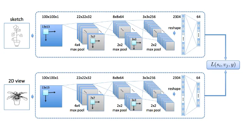
3.2.2 Network architecture

Figure 3.3 shows the architecture of our network for the inputs are views and sketches, respectively. We use the same network design for both networks, but they are learned simultaneously. Our input patch size is 100⇥100 for both sources. The structure of the single CNN has three convolutional layers, each with a max pooling, one fully connected layer to generate the features, and one output layer to compute the cross domain loss.

The first convolutional layer followed by a 4⇥4 pooling generates 32 response maps, each of size 22⇥22. The second layer and pooling outputs 64 maps of size 8⇥8. The third layer has 256 response maps, each is pooled to size 3⇥3. The 2304 features generated by the final pooling operation are linear transformed to 64⇥1 features in the last layer. Rectified linear units are used in all layers.

3.2.3 View definitions and line drawing rendering

This section presents our procedure of generating viewpoints and rendering 3D mod-els. As opposed to multiple best views, we find it sufficient to use two random views to characterize a 3D model because the chance that both views are degenerated is very little. Following this observation, we impose the minimal assumptions on se-lecting views for the whole dataset:

1. Most of the 3D models in the dataset are upright;

2. Two viewpoints are randomly generated for the whole dataset, provided that their angle larger than 45 degree.

Figure 3.4 shows some of our views in the PSB dataset. The first row shows that the upright assumption does not require strict alignments of 3D models, because some models may not have well defined orientation. Further, while the models are upright, they can still have different rotations (second row).

It is worth to stress that this approach does not eliminate the possibility of select-ing more (best) views as input, but the comparisons among view selection methods are beyond the scope of this chapter.

(45)

[image:45.595.172.473.361.470.2]

§3.3 Experiments 29

Figure 3.4: 3D models viewed from predefined viewpoints.

Therefore, we use the following descriptors: 1) closed boundaries and 2) Suggestive Contours [DeCarlo et al., 2003] (Figure 3.5).

(a) Shaded (b) SC (c) Final

Figure 3.5: Line rendering of a 3D model. (a) shaded rendering of the 3D model; (b) the suggestive contour; (c) the combination of shaded contour with suggestive contour.

3 .

3 Experiments

(46)

3.3.1 Datasets

PSB / SBSR dataset The Princeton Shape Benchmark (PSB) [Shilane et al., 2004] is widely used for 3D shape retrieval system evaluation, which contains 1814 3D models and is equally divided into training set and testing set. The 3D models are collected from 161 object classes. Notice that only part of the classes is shared by the training and testing set. To be specific, 21 classes appear in both training and testing set, 69 classes appears only in the training set, and 71 classes are used only for testing. In section 3.3.3, we will evaluate the retrieval performance of the classes exists only in the testing set. As these 3D models are unseen during the training stage, they are more challenging for the similarity learning task.

In [Eitz et al., 2012b], the Shape Based Shape Retrieval (SBSR) dataset is collected for pairing with the PSB 3D models. The 1814 hand drawn sketches were collected using Amazon Mechanical Turk. In the collection process, participants were asked to draw sketches given only the name of the categories, thus the sketches are drawn without any visual clue from the 3D models.

SHREC’13& ’14dataset Although the PSB dataset is widely used in shape retrieval evaluation, there is a concern that the number of sketches for each class in the SBSR dataset is not enough. Some classes have only very few instances (27 of 90 training classes have no more than 5 instances), while some classes have dominating number of instances, e.g., the “fighter jet" class and the “human" class have as many as 50 instances.

To remove the possible bias when evaluation the retrieval algorithms, Li et al. [2014a] reorganized the PSB/SBSR dataset and proposed the SHREC’13 dataset where a subset of PSB with 1258 models was used and the sketches in each class had 80 in-stances. These sketch instances were split into two sets: 50 for training and 30 for testing. Please note, the number of models in each class still varies. For example, the largest class have 184 instances but there are 23 classes having no more than 5 models

(47)

While our performance is still superior (see Figure 3.11 and Table 3.4), we choose to present our results using the SHREC’13 dataset.

Evaluation criteria In our experiment, we use all datasets and measure the per-formance using the following criteria: 1) Precision-recall curve is calculated for each query and linear interpolated, then the final curve is reported by averaging all pre-cision values for fixed recall rates; 2) Average precision (mAP) is the area under the precision-recall curve; 3)Nearest neighbor (NN)is used to measure the top 1 retrieval accuracy; 4)E-Measure (E)is the harmonic mean of the precision and recall for the top 32 retrieval results; 5)First/second tier (FT/ST)andDiscounted cumulated gain (DCG)as defined in the PSB statistics.

3.3.2 Experimental settings

Stopping criteria All three of the datasets had been split into training and testing sets, but no validation set was specified. Therefore, we terminated our algorithm after 50 epochs for PSB/SBSR and 20 for SHREC’13 dataset (or until convergence). Multiple runs were performed and the mean values were reported.

Generating pairs for Siamese network To make sure we generate the reasonable proportion of similar and dissimilar pairs, we used the following approach to gener-ate pair sets. For each training sketch, we random selectedkp view peers in the same category (matched pairs) and kn view samples from other categories (unmatched pairs). Usually, our dissimilar pairs are ten times more than the similar pairs for successful training. In our experiment, we use kp = 2, kn = 20. We perform this random pairing for each training epoch.

Computational cost The implementation of the proposed Siamese CNN is based on the Theano library [Theano Development Team, 2016]. We measured the processing time on a PC with 2.8GHz CPU and GTX 780 GPU. With preprocessed view features, the retrieval time for each query is approximately 0.002 sec on average on SHREC’13 dataset. The code is available from http://users.cecs.anu.edu.au/~fwang/sbsr_prj/sbsr_

demo.html.

(48)

[image:48.595.78.477.92.316.2]

Figure 3.6: Retrieval examples of PSB/SBSR dataset. The cyan denotes the correct retrievals.

3.3.3 Shape retrieval on PSB/SBSR dataset

Examples In this section, we test our method using the PSB/SBSR dataset. First, we show some retrieval examples in Figure 3.6. The first column shows 8 queries from different classes, and each row shows the top 15 retrieval results. The cyan denotes the correct retrievals, and gray denotes incorrect ones.

The method performs exceptionally well in popular classes such as human, face, and plane. We also found that some fine-grained categorizations are difficult to dis-tinguish. For instance, the shelf and the box differ only in a small part of the model. However, we also want to note that some of the classes only differ in semantics (e.g., barn and house only differ in function). Certainly, this semantic ambiguity is beyond the scope of this chapter.

Finally, we want to stress that the importance of viewpoint is significantly de-creased in our metric learning approach. Some classes may exhibit a high degree of freedom such as the plane, but the retrieval results are also excellent (as shown in Figure 3.6).

(49)

Since other methods did not report the results on this dataset, we leave the com-prehensive comparison to the next section. Instead, in this analysis, we focus on the effectiveness of metric learning for shape retrieval.

Table 3.1: Precision-recall on fixed points.

5% 20% 40% 60% 80% 100%

0.616 0.286 0.221 0.180 0.138 0.072

Table 3.2: Standard metrics on the PSB/SBSR dataset.

NN FT ST E DCG mAP

0.223 0.177 0.271 0.173 0.451 0.218

Retrieval for “pure test” classes As we have mentioned before, PSB/SBSR is a very imbalanced dataset, where the training set and the testing set are partially over-lapped. This makes it an excellent dataset for investigating similarity learning be-cause the “unseen” classes verify the learning is not biased to the training classes.

In this experiment, we use the same model trained on the original training and testing split, and evaluate the performance on three different test sets. The “pure test” contains test samples from the classes that never appears in training. The “shared test” contains test samples from the classes that also used in training. The “whole test” consists of all test samples.

Some retrieval examples of the unseen classes are shown in Figure 3.7. It is interesting to see that our proposed method works well even on failure cases, such as the flower, the retrieval returns similar shapes (“potting plant”). This demonstrates that our method learns the similarity effectively. Figure 3.8 shows our comparison on the split testing set according to their class label.

3.3.4 Shape retrieval on SHREC’13and SHREC’14dataset

(50)

Figure 3.7: Retrieval examples of unseen samples in PSB/SBSR dataset. The cyan denotes the correct retrievals.

0 0.2 0.4 0.6 0.8 1

0 0.1 0.2 0.3 0.4 0.5 0.6 0.7

Recall

Precision

Pure test Whole set Shared test

Figure 3.8: Split test set performance on SBSR.

A visualization of the learned features First, a visualization of our learned feature space is presented in Figure 3.9. We perform a principle component analysis on the features learned by our network and reduce the dimension to two for visualization purpose. The green dots denote the sketches, and the yellow ones denote views. For simplicity, we only overlay the sampled views over the point cloud.

While this is a coarse visualization, we can already see some interesting properties of our method. First, we can see that classes with similar shapes are grouped together automatically. On the top right, different animals are mapped to nearby spaces. On the left, various types of vehicles are grouped autonomously. Other examples include house and church, which are very similar.

(51)

[image:51.595.122.513.170.604.2]

(52)

Statistical results This section presents the statistical results on SHREC’13 and SHREC’14. First, we compare the precision-recall curve against the state of the art methods reported in [Li et al., 2014a] and [Li et al., 2014b].

0 0.2 0.4 0.6 0.8 1 0 0.1 0.2 0.3 0.4 0.5 0.6 Recall Precision

Ours Siamese Model

Ours Identic Model

Furuya (CDMR−BF−fGALIF+CDMR−BF−fDSIFT)

Furuya (CDMR−BF−fGALIF)

Furuya (BF−fGALIF+BF−fDSIFT)

Furuya (UMR−BF−fGALIF+UMR−BF−fDSIFT)

Furuya (CDMR−BF−fDSIFT)

Furuya (BF−fGALIF)

Furuya (UMR−BF−fDSIFT)

Li (SBR VC−NUM−100)

Furuya (UMR−BF−fGALIF)

Furuya (BF−fDSIFT)

Li (SBR 2D−3D−NUM−50)

Saavedra (HOG−SIL)

Li (SBR VC−NUM−50)

Saavedra (HELO−SIL)

Saavedra (FDC−CVIU version)

Saavedra (FDC)

Pascoal (HTD)

Aono (EFSD)

Figure 3.10: Performance comparison on SHREC’13. Please refer to [Li et al., 2014a] for the descriptions of the compared methods.

From the Figure 3.10 we can see that our method significantly outperformed other comparison methods. On SHREC’13 benchmark, the performance gain of our method is already 10% when the recall is small. More importantly, the whole curve decreases much slower than other methods when the recall increases, which is desir-able because it shows the method is more stdesir-able. The proposed method has a higher performance gain (30%) when recall reaches 1. Figure 3.11 shows that, on SHREC’14 benchmark, our method consistently shows increased precision as the recall increase (approx. 10%). This demonstrates our method exceeds other methods that use hand-crafted features. The comparison clearly shows that our methods benefited from the learned features a lot, and is much more stable at higher recall level. One rea-son is that the CNN features are more representative than the handcrafted features, thus it is more capable to capture similarities of different classes without loose the discriminative power.

(53)

0 0.2 0.4 0.6 0.8 1

0 0.1 0.2 0.3 0.4 0.5 0.6 Recall Precision Ours

Tatsuma (SCMR−OPHOG) Tatsuma (OPHOG)

Furuya (CDMR (sigma_SM=0.05, alpha=0.3)) Furuya (CDMR (sigma_SM=0.1, alpha=0.3)) Furuya (BF−fGALIF)

Li (SBR−VC (alpha=1))

Furuya (CDMR (sigma_SM=0.05, alpha=0.6)) Li (SBR−VC (alpha=0.5))

Furuya (CDMR (sigma_SM=0.1, alpha=0.6)) Zou (BOF−JESC (Words800_VQ)) Zou (BOF−JESC (FV_PCA32_Words128)) Zou (BOF−JESC (Words1000_VQ))

Figure 3.11: Performance comparison on SHREC’14. Detailed descriptions of the compared methods can be found in [Li et al., 2014b].

both benchmarks. This further demonstrates our method is superior.

[image:53.595.226.407.120.311.2]

We also compared to the case where both networks are identical, i.e., both views and sketches use the same Siamese network. Figure 3.10 suggests that this configu-ration is inferior to our proposed version, but still, it is better than all other methods. This supports our hypothesis that the variations in two domains are different. This also sends a message that using the same features (handcrafted or learned) for both domains may not be ideal.

Table 3.3: Comparison on SHREC’13 dataset. The best results are shown in red, and the second best results are shown in blue.

SHREC’13

NN FT ST E DCG mAP

Ours 0.405 0.403 0.548 0.287 0.607 0.469

Identical Model 0.389 0.364 0.516 0.272 0.588 0.434

From Line Drawings to Human Actions: Deep Neural Networks for Visual Data Representation