arXiv:1407.3910v1 [math.OC] 15 Jul 2014
Approachability in Population Games
∗
Dario Bauso
†Thomas W. L. Norman
‡July 16, 2014
Abstract
This paper reframes approachability theory within the context of pop-ulation games. Thus, whilst one player aims at driving her average payoff to a predefined set, her opponent is not malevolent but rather extracted randomly from a population of individuals with given distribution on actions. First, convergence conditions are revisited based on the com-mon prior on the population distribution, and we define the notion of
1st-moment approachability. Second, we develop a model of two coupled partial differential equations (PDEs) in the spirit of mean-field game the-ory: one describing the best-response of every player given the population distribution (this is aHamilton-Jacobi-Bellman equation), the other cap-turing the macroscopic evolution of average payoffs if every player plays its best response (this is an advection equation). Third, we provide a detailed analysis of existence, nonuniqueness, and stability of equilibria (fixed points of the two PDEs). Fourth, we apply the model to regret-based dynamics, and use it to establish convergence to Bayesian equilib-rium under incomplete information.
1
Introduction
We consider a game played by a large population of individuals in continuous time. At every time, each individual engages in play with a random opponent extracted from the population and the resulting payoff, which depends on the action profiles of both players, is a vector. Such vector payoffs can be interpreted as deriving from a collection of noninterchangeable goods. Let us think, for instance, of a negotiation between an employer and a candidate employee over salary, career prospects, maximal number of days off and so forth. Formally, we can think of the completeness axiom being satisfied along each dimension
∗The work of D. Bauso was supported by the 2012 “Research Fellow” Program of the
Di-partimento di Matematica, Universit`a di Trento and by PRIN 20103S5RN3 “Robust decision making in markets and organizations, 2013-2016”.
†D. Bauso is with Dipartimento di Ingegneria Chimica, Gestionale, Informatica e
Mecca-nica, Universit`a di Palermo, Italy. D. Bauso is currently visiting professor at the Department of Engineering Science, University of Oxford, UK, email:[email protected]
of our vector but failing across them, giving a special case of Aumann’s [4] framework. Indeed, vector payoffs may also be appropriate when the continuity axiom fails (see [12]). Alternatively, each player may be representative of a group of individuals whose preferences may not be aggregated into a single ordering, so that the vector payoff has one component for each individual in the group. Finally, payoff vectors also naturally arise when considering their regret at not having made each possible deviation.
Main results. First, we provide a new model that combines approachability and population games. Given that the opponent is randomly extracted from the population, the approach by Blackwell—which looks at the worst-case payoff— may appear conservative. Thus, we relax Blackwell’s conditions, assuming that the opponent is not malevolent but instead is simply extracted from a popula-tion with given distribupopula-tion; we call this 1st-moment approachability. Second, we build upon the theory of mean-field games and adapt the concept of mean-field equilibrium to our evolutionary set-up; we call this self-confirmed equilibrium. Third, we discuss existence and nonuniqueness of the equilibrium. Finally, we explore the regret interpretation of our model; whereas 1st-moment approacha-bility of nonpositive regrets no longer implies Nash equilibrium (as in [20]), we show that nonpositive maximal regret does imply Bayesian equilibrium under incomplete information.
Related literature. The theory of “approachability” dates back to Blackwell [10] and culminates in the well known Blackwell’s Theorem. Approachability arises in several areas of game theory, such as allocation processes in coalitional games [28], regret minimization [30, 20], adaptive learning [13, 16, 18, 19], ex-cludability and bounded recall [31], and weak approachability [39], just to name a few. For instance, in coalitional games one asks whether the core is an ap-proachable set, and which allocation processes can drive the complaint vector to that set. In regret minimization, one considers the nonpositive orthant in the space of regrets; a player tries to adjust her strategy based on the current regret so as to make that set approachable by the regret vector. Once all players have nonpositive regret, the resulting outcome is an equilibrium for the game. This idea of adapting the new action to the current state of the game is common to adaptive learning and evolutionary games as well, but in regret-based dynamics the state is in payoff (rather than strategy) space. Evolution under incomplete information has been relatively little studied, with the notable exception of Ely and Sandholm [15, 36], who analyse a best response dynamic with a subpopu-lation for each possible type; here, by contrast, we have a single popusubpopu-lation of agents with nonconstant types who adopt (type-dependent) Bayesian strategies through time.
an extension (to a vector space) of the von Neumann minmax theorem [40], the approachability principle also has elements in common with differential inclu-sions [2]. In addition to this, [37] establishes connections with viability theory [1], and set-valued analysis [3] (see, cfg., the comparison between an approach-able set and a discriminating set) and set invariance theory [11].1
The approachability principle is also behind the notion of excludability; along this line, some authors investigate which sets are approachable and which ones excludable under imperfect information (bounded recall, delayed and/or stochastic monitoring) [31]. Connected to approachability as well is the con-cept of “attainability.” Attainability is a new notion developed in [9, 32] in the context of 2-player continuous-time repeated games with vector payoffs. Attainability arises in many contexts such as transportation networks, distribu-tion networks, producdistribu-tion networks applicadistribu-tions. The main quesdistribu-tion is: “Under what conditions does a strategy for player 1 exist such that the cumulative pay-off converges (in the lim sup sense) to a preassigned set (in the space of vector payoffs) independently of the strategy used by player 2?”
A second stream of literature we follow in the present study is the one on mean field games. This theory originated in the work of M. Y. Huang, P. E. Caines and R. Malham´e [23, 21, 22], and independently in that of J. M. Lasry and P. L. Lions [25, 26, 27], where the now standard terminology of Mean Field Games (MFG) was introduced. Explicit solutions in terms of mean field equilibria are not common unless the problem has a linear-quadratic structure, see [8]. Mean field games have connections to evolutionary games (see for instance [24]) and large games [5]. Actually, both theanonymous game
in [24] and thelarge game in [5] build upon the notion of mass interaction and can be seen as a stationary mean field.
This paper is organized as follows. In Section 2, we set up the problem. In Section 3, we provide our population game motivation for the problem at hand. In Section 4, we establish the main results of the paper. In Section 5, we apply the model to a regret-based setting, and show under incomplete information that nonpositive maximal regrets that are approachable in 1st moment must be Bayesian equilibria. Finally, in Section 6, we draw concluding remarks.
Notation. We view vectors as columns. For a vectorx, we usexi to denote its
ith coordinate component. Occasionally we may write (x)i=1,...,mto denote an
m-dimensional column vector. For two vectors xandy, we usex < y (x≤y) to denotexi < yi (xi ≤yi) for all coordinate indicesi. We letxT denote the transpose of a vectorx, and kxkits Euclidean norm. We writeP(x) to denote the projection of a vectorxon a setX, and dist(x, X) for the distance fromx
toX, i.e.P(x) = arg miny∈Xkx−ykand dist(x, X) =kx−P(x)k, respectively. We also denote byconv the convex hull of a given set of points. ∂x indicates the first partial derivative with respect tox.
1Still within the realm of differential games, it is worth noting that the notion of
2
The Model
With the above preamble in mind, the game at hand is a two-player repeated game with vector payoffs in continuous time.2 We assume that the players use nonanticipating behavior strategies with delay. This means that the behavior of a player may depend only on past play. In other words, the way a player plays during a given interval of time does not affect the way the opponent plays during that block. Still, it may affect the other player’s play in subsequent intervals.
LetA={1,2, . . . , n}be a discrete set,ai: [0, T]→Aa measurable function of time andaj : [0, T]→A a random disturbance. Letu:A×A →M where
M = {Mlk, l, k ∈ A} and Mlk ∈ Rm (each entry Mlk is an m-dimensional vector). LetX :=conv{Mlk|l, k∈A}, whereconvdenotes theconvex hull, and consider the differential equation inX
dx(t) =1t(Eu(ai(t), aj(t))−x(t))dt, ∀t∈[0, T],
x(0) =x0∈X, (1)
wherex0 is generated according to a distribution lawρ0(x). More specifically, consider a probability density function ρ : X ×[0,+∞[→ R, (x, t) 7→ ρ(x, t), representing the density of the players whose state isxat timet, which satisfies
R
Rρ(x, t)dx = 1 for everyt. Let us also define the mean state over players at
timetasρ(t) :=R
Xxρ(x, t)dx. We also haveρ(x,0) =ρ0(x).
The objective of a player is to approach a given targety: [0, T]→X. Then, for each group, consider a running costg:X ×X →[0,+∞[, (x, y)7→g(x, y) of the form:
g(x, y) = 1 2
h
(y−x)TQ(y−x)i, (2)
whereQ >0 and symmetric.
The above cost describes i) the (weighted) square deviation of an individual’s state from the target.
Also consider a terminal cost Ψ :X×X →[0,+∞[, (x, y)7→Ψ(x, y) of the form
Ψ(x, y) = 1 2(y−x)
TS(y−x), (3)
whereS >0. The problem in its generic form is then the following:
Problem 1 Let the initial statex(0)be given and with densityρ0.Given a finite
horizonT >0, a suitable running cost: g:X×X →[0,+∞[,(x, y)7→g(x, y), as in (2); a terminal cost Ψ : X×X →[0,+∞[, (y, x)7→ Ψ(y, x), as in (3), and given a suitable dynamics forxas in (1), solve
inf ai(·)∈C
(
J(x0, ai(·), aj(·)) =
Z T
0
g(x(t), y)dt+ Ψ(x(T), y)
)
, (4)
2Whilst the game is repeated, opponents are constantly rematched, and hence no
whereCis the set of all measurable functionsai(·)from[0,+∞[toAi, andEu(·) in (1) must be consistent with the evolution of the distributionρ(·)if every player behaves optimally.
3
Motivation: Population Games
Consider a population game where continuously in time every individual matches with an opponent randomly extracted from the population and the resulting payoff is a vector. The resulting game is a two-player repeated game with vec-tor payoffs in continuous time Γ that every individual plays against a population with given (evolving) distribution over actions. Let A be the finite set of ac-tions of every individual, then the instantaneous payoff is given by a function
u:A×A→Rm, wherem is a natural number. We assume w.l.o.g. that pay-offs are bounded and correspond to the elements of the following discrete set
M ={Mlk, l, k∈A}whereMlk∈Rm, so thatu:A×A→M. We extenduto the set of mixed-action pairs, ∆(A)×∆(A), in a bilinear fashion. The one-shot vector-payoff game (A, A, u) is denoted byGand we will say that the game in continuous time Γ isbased on G.
The game Γ is played over the time interval [0,∞). We assume that the players use markovian strategies
σ:X×[0, T]→A such that ai(t) :=σ(x, t),
whereX :=conv{Mlk|l, k∈A}andxis the average (over time) expected (over opponent’s play) payoff defined as:
x(t) = 1
t
Z t
0
Eu(ai(t), aj(t))dt∈Rm (5)
In the above equation,
Eu(ai(t), aj(t)) := u(ai(t), q(t))
q∈∆(A) s.t. qk =RRkρ(x, t)dx,
Rk :={x∈Rm|σ(x, t) =k},∀k∈A.
(6)
Once we differentiate (5) with respect totwe obtain the equation (1) in the same spirit as in Hart and Mas-Colell’s paper [20] on continuous-time approach-ability. Then, Problem 1 analyzes the approachability of a given target in the space of vector payoffs on the part of a population of individuals.
Example 1 (Prisoners’ Dilemma)Suppose, for instance, that players target the average payoffs across the population. Consider the following game:
Cooperate Defect Cooperate (3,3) (0,4)
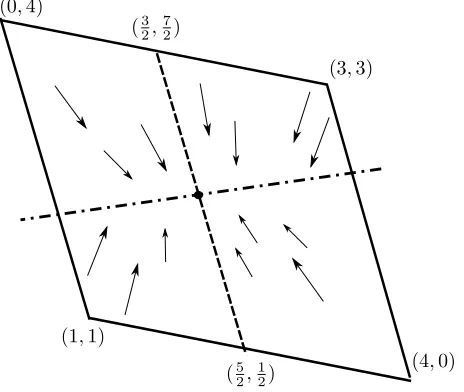
Figure 1 depicts the payoff space in the continuous-time game based on this Pris-oner’s Dilemma. Here, the state space is X =conv{(3,3),(1,1),(0,4),(4,0)}
(the boundary is in solid line), and the targetyis the barycenter assuming a uni-form distribution. One can visualize the supporting hyperplane H (dot-dashed line) passing through the barycenter, and the vector field dx(t) converging to
(32,72) for those who cooperate (region below H) and to (52,12) for those who defect (region aboveH). The set conv{(32,72),(52,12)} is the set of approachable points with population strategyq= ((1
2, 1 2),(
1 2,
1
2)), and the barycenter is at the
equilibrium with uniform distribution overX. This will be explained in Theorem 2.
(1,1)
(4,0) (0,4)
(3,3) (32,72)
(52,12)
Figure 1: Payoff space of Prisoners’ dilemma: State space X =
conv{(3,3),(1,1),(0,4),(4,0)}(boundary in solid line), supporting hyperplane
H (dot-dashed line) passing through the barycenter, vector fielddx(t) converg-ing to (32,72) for those who cooperate (region below H) and to (52,12) for those who defect (region aboveH),conv{(32,72),(52,12)} is set of approachable points with population strategyq = ((1
2, 1 2),(
1 2,
1
2)), barycenter is self-confirmed with uniform distribution overX.
4
Main results
This section outlines the main results of this paper. After introducing the
4.1
Expected value of the projected game
Given the above game, we wish to analyze convergence properties in the space of distributions of the cumulative or average payoff xi(t), in the spirit of ap-proachability. We will make use of the notion ofprojected game which we recall next. Letλ∈Rm and denote byhλ, Githe one-shot zero sum game whose set of players and their actions are as in gameG, and the payoff that playerj pays to playeri isλTu(a
i(t), aj(t)) for every (ai(t), aj(t))∈Ai×Aj. Observe that, as a zero-sum one-shot game, the gamehλ, Gihas avalue, val(λ), obtained as
val(λ) := min ai(t)
max aj(t)
λTu(ai(t), aj(t)).
Given the stochastic nature ofaj(t) the above min-max operation is not useful to our purposes. Then, we rather consider the expected value of the game (where the inner maximization is replaced by an expectation) and discuss approacha-bility in expectation. In the light of this, and using the bilinear structure of the utility function, and assuming markovian strategies
σ:X×[0, T]→A such that ai(t) :=σ(x, t)
we can rewrite the expected value as
Eval(λ) := minai(t)EλTu(ai(t), aj(t)) = minai(t)λTu(ai(t), q(t)),
q∈∆(A) s.t. qk=RRkρ(x, t)dx,
Rk:={x∈Rm|σ(x, t) =k},∀k∈A.
(7)
In the case of state-dependent payoff, which occurs when we consider the game whose payoff is
f(u(ai(t), aj(t)), x(t)) = 1
t(Eu(ai(t), aj(t))−x(t)) =
1
t(u(ai(t), q(t))−x(t)),
the above expression can be modified as:
Evalx(λ) := minai(t)EλTf
u(ai(t), aj(t)), xi)
= minai(t)λTf
u(ai(t), q(t)), xi
q∈∆(A) s.t. qk=RRkρ(x, t)dx,
Rk:={x∈Rm|σ(x, t) =k},∀k∈A.
(8)
Note that here we use the notationu(ai(t), q(t)) to meanEu(ai(t), aj(t)).
4.2
Approachability in 1st-moment
To introduce the approachability principle, let Φ be a closed and convex set in Rm and let P(x) be the projection of any pointx∈Rm (closest point to x
in Φ).
Definition 1 (Approachable set) A closed and convex setΦinRmis approach-ableby player 1 if there exists a strategy for player 1 such that (9) holds true for every strategy of player 2:
lim
t→∞dist(x(t),Φ) = 0. (9)
The next result is the Blackwell approachability theorem.
Proposition 1 (Approachability principle [10, 33]) A closed and convex setΦ
in Rm is approachable by player 1 if for every x(t) there exists a strategy for player 1 such that (10) holds true for every strategy of player 2:
[x(t)−P(x(t))]T[x(t)−P(x(t)) +f(u
i(σ(x, t), aj(t)), xi(t))]≤0, ∀ t. (10)
Note that in the above statement, condition (10) is equivalent to saying that i) for everyxtakingλ= kxx−−PP((xx))k∈Rmthe value of the projected game satisfies
[x(t)−P(x(t))]T[x(t)−P(x(t))] +kx−P(x)kval
x(λ)≤0, ∀t. (11)
Now, if we assume that the opponent is committed to play a mixed strategy
q∈∆(A), condition (10) turns into
[x(t)−P(x(t))]T[x(t)−P(x(t)) +f(u(σ(x, t), q(t)), x(t))]≤0, ∀t, (12)
and the corresponding condition (11) can be rewritten as
[x(t)−P(x(t))]T[x(t)−P(x(t))] +kx−P(x)kEval
x(λ)≤0, ∀t,
Evalx(λ) := minai(t)λTf(ui(ai(t), q(t)), xi). (13)
Theorem 1 (Approachability in1st-moment)Letq∈∆(A)be given. The set of approachable targets is
T(q) ={y| y= X l,k∈A
plqkMlk,∀p∈∆(A)}.
Furthermore, there exists a partitioningR1, . . . , Rn such that the approachable strategies are markovian and bang-bang:
σ(x) =
ai=k if x∈Rk :={ξ|(ξ−y)T(u(k, q)−y)≤0}
ai6=k otherwise. (14)
Proof. Sketch. (sufficiency) Let y ∈ T(q). Rewrite as y = P
Then for every x∈X, taking λ= kxx−−yyk ∈Rm the value of the projected game satisfies
(
[x(t)−y]T[x(t)−y] +kx−ykEval
x(λ)≤0, ∀t.
Evalx(λ) := minai(t)λTf
u(ai(t), q(t)), x
(15)
(necessity) Lety6∈ T(q). Then the above does not hold. Q.E.D.
In the problem at hand, one additional challenge is that q must be self-confirmed. This means that the mixed strategyq entering the computation of the expected value of the projected games Evalx(λ) must reflect the current state distribution. In formulas, this corresponds to expanding (15) as follows:
[x(t)−y]T[x(t)−y] +kx−ykEval
x(λ)≤0, ∀t.
Evalx(λ) := minai(t)λTf
u(ai(t), q(t)), x
q∈∆(A)s.t. qk=
R
Rkρ(x, t)dx,
Rk :={ξ|(ξ−y)T(u(k, q)−y)≤0} ∀k∈A.
(16)
In the rest of the paper we look for self-confirmed solutions, which we call equilibria.
4.3
The mean field game
Let us denote by v(x, t) the value of the optimization problem starting from time t at state x. The first step is to show that the problem results in the following mean field game system for the unknown scalar functionsv(x, t), and
ρ(x, t) when each group behaves according to (4):
∂tv(x, t) + inf ai
{f(u(ai, q), x)∂xv(x, t) +g(x, y)}= 0 inRm×[0, T[,
v(x, T) = Ψ(x, y)∀x∈Rm,
∂tρ(x, t) +div(ρ(x, t)·f(u(a∗i, q), x)) = 0,
ρ(0) =ρ0,
(17)
where a∗
i(t, x) and q are the optimal time-varying state-feedback controls of playersiandj, respectively, obtained as
a∗
i =σ(x)∈arg minai∈Ai{f(u(ai, q), x)∂xv(x, t) +g(x, y)},
q∈∆(A)s.t. qk =RRkρ(x, t)dx,
Rk :={x∈Rm|σ(x) =k},∀k∈A.
(18)
Given the boundary condition on final state (second equation in (17)), and assuming a given population behavior captured by ρ(·), the HJB equation is solved backwards and returns the value function and best-response behavior of the individuals (first equation in (18)) as well as the worst adversarial response (second equation in (18)). The HJB equation is coupled with a second PDE, known as Fokker-Planck-Kolmogorov (FPK) (third equation in (17)), defined on variableρ(·) and parametrized inv(x, t). Given the boundary condition on initial distributionρ(0) = ρ0 (fourth equation in (17)), and assuming a given individual behavior described by u∗, the FPK equation is solved forward and
returns the population behavior time evolutionρ(t).
Let condition (12) hold true. Now, for givenx, take forλthe valueλ(∂xv) = ∂xv(x,t)
k∂xv(x,t)k which is the gradient direction on x. Then, we can introduce the expected value of theprojected anti-gradient game
Evalx[∂xv(x, t)] :=λ(∂xv)Tf(ui(a∗i, q), x). We can then establish the following result.
Theorem 2 (Self-confirmed equilibria)Let condition (12) hold true. Then, the mean-field game formulation of Problem 1 is
∂tv(x, t) +k∂xvkEvalx[∂xv] +21(y(t)−x)TQ(y(t)−x) = 0,
inRm×[0, T[,
v(x, T) = Ψ(y(T), x), in Rm,
∂tρ(x, t) +div(ρ(x, t)·f(ui(a∗i, q)) = 0, in Rm×[0, T[,
ρ(x,0) =ρ0(x)inRm.
(19)
Furthermore, the optimal controls for players 1 and 2 are
a∗
i =σ(x)∈arg minai∈Aiλ(∂xv) Tf(u(a
i, q), x)
q∈∆(A)s.t. qk =RRkρ(x, t)dx,
Rk :={ξ|(ξ−y)T(u(k, q)−y)≤0} ∀k∈A,
σ(x) =k,such that x∈Rk.
(20)
Proof. Due to the bilinear structure of f, we can deduce that the best-response strategy u∗ and worst adversarial disturbance w∗ are on a vertex of
We can rewrite the value of the anti-gradient projected game as
Evalx[∂xv] = inf l∈A
X
k∈A 1
t(qkMlk−x)
Tλ(∂ xv),
Best responses and adversarial strategies are then given by
a∗i = arg min l∈A
X
k∈A 1
t(qkMlk−x)
Tλ(∂ xv).
With the above definition ofEvalx[∂xv] in mind, the Hamilton-Jacobi part of (17) can be rewritten as
∂tv+k∂xvkEvalx[∂xv] + 1
2(y(t)−x(t)) T
Q(y(t)−x(t)) = 0 inRm×[0, T[, v(x, T) = Ψ(x)∀x∈Rm.(21)
It is left to observe that f(u∗, w∗) =Ai∗j∗ and proves the third equation (FPK equation). Q.E.D.
In principle, to find the optimal control input we need to solve the two coupled PDEs in (19) inv andρ with given boundary conditions (second and last conditions).
4.4
Existence and nonuniqueness of equilibria
In this section we investigate existence and nonuniqueness of equilibria. To do this, we analyze the time-dependence of an estimate errorν(t), which accounts for the deviation between an estimated density q(t) and a current one ˜q(t) at timet:
ν(t) =q(t)−q˜(t),
where
q˜
k(t) =RRkρ(x)dx
Rk:={ξ|(ξ−y(t))T(u(k, q)−y(t))≤0}.
(22)
Observe that the time-dependence of ˜q(t) enters in the above through the time-varying nature of the targety(t). Now, according to our procedure, we wish to hypothesize a pair (p, q), which constitutes the input, and obtain a new density ˜
q(p, q) as an output. To see this, from y =P
l,k∈AplqkMlk,∀p, q ∈∆(A) the expression (22) can be rewritten as
q˜
k(p, q) =
R
Rkρ(x)dx,
Rk:={ξ|(ξ−Pl,k∈AplqkMlk)T(u(k, q)−
P
l,k∈AplqkMlk)≤0}.
(23)
Eventually, the procedure should return a fixed point. In other words, if we think of an equilibrium as the pair (p∗, q∗) such that ν(p∗, q∗) = 0, existence
of an equilibrium is now related to existence of a fixed point for the above procedure, i.e.,
˜
The above means that, given a (p, q) as input to our procedure, the output ˜
q(p, q) coincides with the hypothesized densityq. It is natural to represent the above algorithmic procedure, as a continuous-time dynamical system and thus to relate convergence to a fixed point to the asymptotic stability of the dynamics. The next assumption introduces conditions for the asymptotic stability to hold.
Assumption 1 There exists a pair ( ˙p,q˙)such that
−∂pq˜1p˙+ ˙q1−∂qq˜1q˙
.. .
−∂pq˜ip˙+ ˙qi−∂qq˜iq˙ ..
.
−∂pq˜mp˙+ ˙qm−∂qq˜mq˙
:= (−∂pq˜ip˙+ ˙qi−∂qq˜iq˙)i=1,...,m≤ −κ(q−q˜). (24)
The above describes the possibility of varying (p, q) in order to reduce the es-timate error ν, whatever the current error is. The next result establishes the existence of an equilibrium based on the above condition.
Theorem 3 (existence) Let Assumption 1 hold. Then, the estimate error decays exponentially fast, i.e.
ν(t)≤e−κtν(0).
Proof. This proof is based on a Lyapunov stability approach. In particular, let us introduce a quadratic (in the error) Lyapunov function
L=1 2ν
Tν,
and show that its derivative is strictly negative. The time derivative can be decomposed as sum of two terms involving the gradient ofLwith respect to the two variablespandq. More specifically,
˙
L= (∂pL)Tp˙+ (∂qL)Tq˙ =νTν˙ = (q−q˜)Th (∂
pνi)Tp˙
i=1,...,m+ (∂qνi) Tq˙
i=1,...,m
i
= (q−q˜)T(−∂
pq˜ip˙+ ˙qi−∂qq˜iq˙)i=1,...,m.
(25)
From condition (24), we also have ˙
L ≤ −κ(q−q˜)T(q−q˜) =−κνTν,
which proves the thesis. Q.E.D.
Essentially the above theorem shows that if we let the algorithm run for a long time the estimate error asymptotically converges to zero, namely,
lim t→∞ν= 0,
which proves the existence of an equilibrium.
Theorem 4 (nonuniqueness)Starting at an equilibrium where L= 0, if for allλ∈Rm,kλk= 1we have
minp,˙q˙λTν˙ = minp,˙q˙λT(−∂pq˜ip˙+ ˙qi−∂qq˜iq˙)i=1,...,m
<0<maxp,˙q˙λTν˙ = maxp,˙q˙λT(−∂pq˜ip˙+ ˙qi−∂qq˜iq˙)i=1,...,m, (26)
then there exists a ( ˙p,q˙) such that L˙ = 0 and thus the current equilibrium is nonunique.
Proof. There exists a ( ˙p,q˙) such that
˜
q(p+ ˙pdt, q+ ˙qdt) =q+ ˙qdt.
The above also means that the error
ν= ˜q(p+ ˙pdt, q+ ˙qdt)−(q+ ˙qdt) = 0.
Q.E.D.
4.5
Solution of the mean field game
This section investigates on the microscopic dynamics of every player given an equilibrium (p, q) and the corresponding target which is common prior, where the target is denoted by
y= X l,k∈A
plqkMlk.
As a result we obtain that such a dynamics is a “potential” one, in the sense that every player’s current average payoff, which we can callstateof the player, describes a trajectory along the anti-gradient of a potential function, the latter being the value function of the mean-field game introduced earlier. To this purpose, let us denote by e(t) the deviation between the target y that every player wishes to approach, and the current average payoffx(t), namely
e(t) =y−x(t).
Given that our running cost is quadratic, from dynamic programming, it is natural to assume that the value function has also a quadratic structure. This is a recurrent approach which needs an a posteriori verification of the consistency of the quadratic assumption. In particular, let us assume that the upper bound for the value function takes the form
ϕ(x, t) = 1 2e
TΦ
te, (27)
where Φtis an opportune matrix which is positive definite, i.e., Φt>0. Likewise, consider a quadratic function for the terminal penalty, namely,
Ψ(x) =1 2e(T)
Then, the HJB equation in (29) can be rewritten as
∂tϕ(x, t) +k∂xϕ(x, t)kEvalx[∂xϕ(x, t)] + 1 2e(t)
TQe(t) = 0 in
Rm×[0, T[, ϕ(x, T) = Ψ(x)∀x∈Rm. (28) Substituting the expression (27) for the value function in (28) we obtain
1 2e(t)
T˙Φ te(t)−
1 2e(t)
TΦ te(t) +
1 2e(t)
TQe(t) = 0 inRm×[0, T[, 1
2e(T) TΦ
Te(T) = Ψ(x)∀x∈Rm. (29) The advantage of writing the HJB as above is in that all terms are explicitly written as quadratic terms in the errore(t). Considering that the HJB has to hold true for everye(t), we can drope(t) and thus we have an expression in the only matrix variable Φtas displayed next:
˙
Φt−Φt+Q= 0 in [0, T[, ΦT =ψ∀x∈Rm.
The above has the form of a classical differential Riccati equation which can be solved backwardly given the boundary conditions on the matrix in the terminal penalty, ΦT =ψ. We can use such a result to analyze the microscopic dynamics of each player as detailed in the next subsection.
4.5.1 Microscopic model
Every single player is characterized by the following system of equations involv-ing the evolution of the average payoff (first equation), its best-response (second equation), and the expression for the density (third equation):
dx(t) =1t P
k∈AqkMa∗k−x(t)
dt, a∗(x, t) = arg min
a∈A(Φte(t))T Pk∈AqkMak−x(t),
q∈∆(A)s.t. qk =RRkρ(x, t)dx,
Rk :={x∈Rm|σ(x, t) =k},∀k∈A.
(30)
Note that the expression for the best-response is obtained from (20) where∂xv is now replaced by Φte(t). This is a straightforward consequence from assuming the value function quadratic as in (27).
Lett=es then
˙
x(s) =X k∈A
qkMa∗k−x(s) =u(a∗, q)−x(s).
For all x the supporting hyperplane H := {ξ|(ξ−y)T(u(a∗, q)−y) = 0}
separatesxfromu(a∗, q), i.e.,
(x−y)T(u(a∗, q)−y) = (x−y)T(X
k∈A
qkMa∗k−y)≤0.
5
Application: Regret and Bayesian equilibrium
Perhaps the leading application of games with vector payoffs is in the study of regret-based dynamics, to which we now turn.
5.1
Regret targeting in classical two-player games
Given a symmetric normal-form game with common action setAand symmetric payoff function π : A → R, let the regret of player i from not having played actionk∈Aunder action profileα∈A2 be
r(k, α) =π(k, α−i)−π(αi, α−i).
A straightforward way to justify the vector payoffs introduced earlier is to make them coincide with the regret vector associated to each action profile, i.e.
u(α) :=r(k, α) k∈A.
In Hart and Mas-Colell [20], approachability of the nonpositive orthant implies convergence to Nash equilibrium under such payoffs. This is no longer true for 1st-moment approachability, which drives expected—rather than maximum— regret to zero, so that some deviations could still have positive regret.
In the following, we turn standard games like the Prisoners’ Dilemma, coor-dination games and Hawk–Dove games into games with regret vectors of type
Left Right
Top
0
a
0
b
Bottom
−a
0
−b
0
and analyse the resulting dynamics of a population targeting expected regret.
Example 2 (Prisoners’ Regret) Consider again the Prisoners’ Dilemma, and the following bimatrix, which represents the regret vector of player 1:
Cooperate Defect
Cooperate
0 1
0 1
Defect
−1 0
−1 0
fromCtoDhe would earn a payoff of1, in comparison with a regret of0when sticking to C. This is represented by the regret vector (0,1)for the action pro-file(C, D). The reasoning would be analogous if Column were to play C. Note that at the pure Nash equilibrium (D, D) the regret vector is component-wise nonpositive.
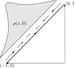
(−1,0)
(0,1)
ρ(x,0)
Figure 2: Regret space of Prisoners’ dilemma: State space X =
[image:16.612.237.394.198.340.2]conv{(−1,0),(0,1)}(solid line), initial distributionρ(x,0) (grey area), and vec-tor fielddx(t) converging toy= (−0.5,0.5).
Figure 2 depicts the state spaceX =conv{(−1,0),(0,1)} (solid line) in the case with an initial distributionm(x,0)(grey area) of players. The arrows indi-cate the vector fielddx(t)if every player in statex∈conv{(−1,0),(−1/2,−1/2)}
cooperates, i.e.ai = 1and every player in statex∈conv{(0,1),(−1/2,−1/2)} defects. The vector field is such that eventually all players converge to the targety = (−1/2,1/2). Consequently, the distribution converges asymptotically to a Dirac impulse iny.
Example 3 (Coordination game) Consider now the coordination game in the bimatrix on the left, with associated regret-vector game on the right:
Mozart Mahler Mozart (2,2) (0,0)
Mahler (0,0) (1,1)
Mozart Mahler
Mozart
0
−2
0 1
Mahler
2 0
−1 0
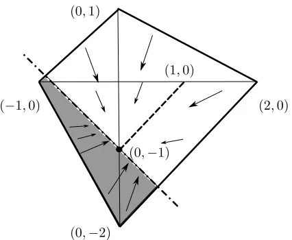
In Fig. 3 we illustrate the state space X =conv{(−1,0),(0,1),(0,−2),(2,0)}
(the boundary is in solid line). With a target y = (0,−1), suppose we have a distribution on actions q= (2/3,1/3), i.e. 2/3 of the population plays Mozart, thenu(1, q) = (0,−1) andu(2, q) = (1,0) (herek = 2 means playing Mahler). The set of approachable points with mixed population strategy q = (2/3,1/3)
(0,−2)
(−1,0) (2,0)
(0,1)
(1,0)
[image:17.612.203.416.119.294.2](0,−1)
Figure 3: Regret space of the coordination game: State space X =
conv{(−1,0),(0,1),(0,−2),(2,0)} (boundary in solid line), and vector field
dx(t) converging to (1,0) (grey area) and (0,−1) (white area), approachable point isy= (0,−1), set of approachable points isconv{(1,0),(0,−1)}(dashed line) with mixed population strategyq= (23,13).
dx(t) if every player in state x ∈ R2 := {ξ|(ξ−y)T(u(2, q)−y) ≤ 0} (grey
area) plays Mahler, namely,ai=σ(x) = 2. On the other hand, every player in statex∈R1:={ξ|(ξ−y)T(u(1, q)−y)≤0}(white area) plays Mozart, namely,
ai=σ(x) = 1. Obviously we need that the integral of the distributionmoverR2
is consistent with the initial assumption, which meansq2=RR
2ρ(x, t)dx= 1/3.
If this occurs, the vector field is such that eventually all players converge to y= (0,−1). Consequently, the distribution converges to a Dirac impulse iny.
Example 4 (Hawk–Dove game) We can likewise transform the Hawk–Dove (or chicken) game on the left into the corresponding regret-vector game on the right:
Hawk Dove
Hawk −1,−1 (4,0)
Dove (0,4) 2,2
Hawk Dove
Hawk
0 1
0
−2
Dove
−1 0
2 0
We have two pure Nash equilibria (Dove, Hawk) and (Hawk, Dove), whose corresponding regret vectors are nonpositive.
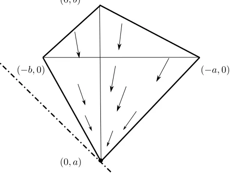
More generally, let us now consider the parametric game introduced earlier:
Left Right
Top
0
a
0
b
Bottom
−a
0
−b
0
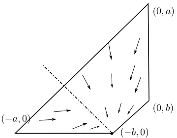
Fig. 4 illustrates the state space X = conv{(0, a),(−a,0),(−b,0),(0, b)} (the boundary is in solid line) where a < 0 < b. The target y = (0, a) is in the negative orthant. Here we consider a distribution on actions q = (1,0), i.e. everybody playsk= 1, thenu(1, q) = (0, a) andu(2, q) = (−a,0). The arrows indicate the vector fielddx(t) for which eventually all players converge to y = (0, a). Consequently, the distribution converges to a Dirac impulse iny. Note that the supporting hyperplaneH:={ξ|(ξ−y)T(u(2, q)−y) = 0}(dot-dashed line) intersectsXat only one point (the vertex), which is proven to be necessary for the vertex to be at the equilibrium. This will be explained in Theorem 2.
(0, a)
(−b,0) (−a,0)
(0, b)
Figure 4: Regret space of parametric game with a < 0 < b: State space
X = conv{(0, a),(−a,0),(−b,0),(0, b)} (boundary in solid line), vector field
dx(t) converging to (0, a) which is also an approachable vertex with population strategy q = (1,0), supporting hyperplane H (dot-dashed line) intersects X
only in one point (the vertex).
Fig. 5 depicts the state space X =conv{(0, a),(−a,0),(−b,0),(0, b)} (the boundary is in solid line) where 0 < b < a. The target y = (−b,0) is again in the negative orthant. Here we consider a distribution on actionsq= (0,1), i.e. everybody plays k = 2, then u(1, q) = (0, b) and u(2, q) = (−b,0). The arrows indicate the vector field dx(t) for which eventually all players converge to y = (−b,0). Consequently, the distribution converges to a Dirac impulse in y. However, there is an issue here related to the fact that the vertex y is not at the equilibrium. To see this, note that the supporting hyperplaneH :=
(0, b) (0, a)
(−a,0)
[image:19.612.222.402.122.263.2](−b,0)
Figure 5: Regret space of parametric game with 0 < b < a: State space
X=conv{(0, a),(−a,0),(−b,0),(0, b)}(boundary in solid line), supporting hy-perplane H (dot-dashed line) passing through the vertex (−b,0), vector field
dx(t) converging to (0, b) left ofH and to (−b,0) right ofH,conv{(0, b),(−b,0)}
is set of approachable points with population strategyq= (0,1), vertex (−b,0) is not self-confirmed, while vertex (0, a) is self-confirmed with population strategy
q= (1,0).
5.2
Maximum regret and Bayesian equilibrium
Whilst 1st-moment approachability gives interesting dynamics in population games based on regret then, it does not give convergence to Nash equilibrium. In this section, however, we show how the model can be applied to an incomplete-information setting to yield convergence to Bayesian equilibrium.
Suppose then that the continuous-time population game Γ is based on a game of incomplete information; in particular, we are given a Harsanyi game
G(as described in [41]) with state of the worldω= (s(ω);t1(ω), t2(ω)) chosen by Nature from a finite set Y using a probability distribution θ. Players then learn their own types ti(ω) ∈ Ti, choose actions βi from a common finite set
B(ω), and receive symmetric payoffs̟i(β;ω),β= (β1, β2); the state of nature iss(ω) = (B(ω), ̟),̟= (̟1, ̟2). Each playerithen has a common finite set Σ of (Ti-measurable) pure Bayesian strategiesσi:Y →B(ω), which we identify with the action setAin our general framework. Given a strategy profileσ∈Σ2, let the vector payoffs be given bymaximal regrets,
u(σ) :=max
k∈Σr(k(ω), σ(ω))
ti∈Ti
.
Players are continuously rematched against new opponents to play this game
in Γ then implies that
Eθmax
k∈Σ̟i(k(ω), σ−i(ω))−̟i(σ(ω))≤0.
But since the maximum of convex functions is convex, Jensen’s inequality im-plies that the left-hand side is no less than
max
k∈ΣEθ̟i(k(ω), σ−i(ω))−Eθ̟i(σ(ω)),
which is hence also nonpositive. Thus, we have a Nash equilibrium of the Harsanyi game, which is also a Bayesian equilibrium of the incomplete-information game by Harsanyi’s [17] Theorem I.
For example, consider a game Gwhere each player’s payoffs are randomly determined; with probability 1/2, the Row playerR has the payoffs in the left-hand “l” matrix, and with probability 1/2, she has the payoffs in the right-hand “h” matrix:
l Opera Football
Opera 3 1
Football 0 2
h Opera Football
Opera 1 3
Football 2 0
The Column playerC’s payoffs are determined in a symmetric manner. Each player observes her own payoffs, but not those of her opponent. There are thus four possible states of the worldY ={ωll, ωlh, ωhl, ωhh}:
ωll= sll; [12ωll,12ωlh],[12ωll,12ωhl]
ωlh= slh; [12ωll,12ωlh],[12ωlh,12ωhh]
ωhl= shl; [12ωhl,12ωhh],[12ωll,12ωhl]
ωhh= shh; [12ωhl,12ωhh],[12ωlh,12ωhh],
(31)
each occurring with probability 1/4. Furthermore, there are two possible types of each player,
{Rl, Rh}=
1 2ωll,
1 2ωlh
,
1 2ωhl,
1 2ωhh
,
{Cl, Ch}=
1
2ωll, 1 2ωhl
,
1
2ωll, 1 2ωhl
,
and each player assigns probability 1/2 to each of her opponents’ possible types. Representing this situation as a Bayesian game, the Row player’s vector payoffs are:
Ol,Oh Ol,Fh Fl,Oh Fl,Fh
Ol,Oh
3 1 2 2 2 2 1 3
Ol,Fh
3 2 2 1 2 1 1 0
Fl,Oh
0 1 1 2 1 2 2 3
Fl,Fh
where, for example, Ol, Fh denotes the pure Bayesian strategy {σR(Rl) =
{Opera}, σR(Rh) ={Football}}. The Column player’s payoffs are symmetric. This game has one pure-strategy equilibrium where Row playsOl,Fh and Col-umn playsOl, Oh, and a symmetric one where Row playsOl,Oh and Column playsOl,Fh.
Now convert this game into one with maximal-regret payoffs:
Ol,Oh Ol,Fh Fl,Oh Fl,Fh
Ol,Oh
0 1 0 0 0 0 1 0
Ol,Fh
0 0 0 1 0 1 1 3
Fl,Oh
3 1 1 0 1 0 0 0
Fl,Fh
3 0 1 1 1 1 0 3
For instance, if Row is playing Fl, Oh and Column is playing Ol, Oh, Row type Rl’s expected payoff is 0, whereas he could have had 3 by playing Ol,
Oh, giving a maximal regret of 3; similarly, typeRh’s payoff is 1, whereas he could have had 2 by playingFl,Fh, giving a maximal regret of 1. 1st-moment approachability of the nonpositive orthant with these maximal-regret payoffs then implies Bayesian equilibrium.
In this respect, from Theorem 1 we know that, for instance, for any pure strategyq we have
T(q) =
{y| y∈conv((0,1),(0,0),(3,1),(3,0))}, q= (1,0,0,0),
{y| y∈conv((0,0),(0,1),(1,0),(1,1))}, q= (0,1,0,0),
{y| y∈conv((0,0),(0,1),(1,0),(1,1))}, q= (0,0,1,0),
{y| y∈conv((1,0),(1,3),(0,0),(0,3))}, q= (0,0,0,1).
(32)
This means that for any pure strategyq the origin (0,0) is reachable and in particular the corresponding strategy is
σ(x) =
ai= 2 for allx, q= (1,0,0,0),
ai= 1 for allx, q= (0,1,0,0),
ai= 1 for allx, q= (0,0,1,0),
ai= 3 for allx, q= (0,0,0,1).
(33)
6
Conclusion
This paper has combined approachability theory, evolutionary games, and mean-field games in a unified framework. The game studied has a vector payoff, a large number of players, and admits classical mean-field game representation involv-ing two coupled PDEs, theHamilton-Jacobi-Bellman equationand theadvection equation. We have highlighted multiple contributions. First, we coin the no-tion of1st-moment approachability and analyze the corresponding convergence conditions. Second, we use the mean-field game to introduce theself-confirmed equilibrium. Third we discuss on existence, non uniqueness, and stability of equilibria as fixed points of the two PDEs.
Future work involves the stochastic analysis of the same game in the pres-ence of an additional Brownian motion in the dynamics. This would capture uncertainty or model-misspecification. In a different direction, we are interested in extending the study to the case where each player can adopt a mixed strat-egy, which would imply a new definition of density distribution on the space of mixed strategies; so far, the density distribution is defined on the space of pure strategies. A third development will be a further analysis of the connections with the Bayesian approach.
References
[1] J. P. Aubin. Viability Theory. Birkh¨auser, 1991.
[2] J. P. Aubin and A. Cellina. Differential Inclusions: Set-Valued Maps and Viability Theory. Springer, 1991.
[3] J. P. Aubin and H. Frankowska. Set-Valued Analysis. Birkh¨auser, 1990.
[4] R. J. Aumann. Utility theory without the completeness axiom. Economet-rica, 30:445–462, 1962.
[5] R. J. Aumann. Markets with a continuum of traders. Econometrica, 32(1-2):39–50, 1964.
[6] Robert J. Aumann and Michael B. Maschler.Repeated Games with Incom-plete Information. MIT Press, 1995.
[7] F. Bagagiolo and D. Bauso. Objective function design for robust optimality of linear control under state-constraints and uncertainty. ESAIM: Control, Optimisation and Calculus of Variations, 17:155–177, 2011.
[8] M. Bardi. Explicit solutions of some linear-quadratic mean field games.
Network and Heterogeneous Media, 7:243–261, 2012.
[10] D. Blackwell. An analog of the minimax theorem for vector payoffs.Pacific J. Math., 6(1):1–8, 1956.
[11] F. Blanchini. Set invariance in control a survey.Automatica, 35(11):1747– 1768, 1999.
[12] L. E. Blume, A. Brandenburger, and E. Dekel. Lexicographic probabilities and choice under uncertainty. Econometrica, 59(1):61–79, 1991.
[13] N. Cesa-Bianchi and G. Lugosi. Prediction, Learning and Games. Cam-bridge University Press, 2006.
[14] N. J. Elliot and N.J. Kalton. The existence of value in differential games of pursuit and evasion. J. Differential Equations, 12:504–523, 1972.
[15] Jeffrey C. Ely and William H. Sandholm. Evolution in bayesian games i: Theory. Games and Economic Behavior, 53:83–109, 2005.
[16] D. Foster and R. Vohra. Regret in the on-line decision problem. Games and Economic Behavior, 29:7–35, 1999.
[17] John C. Harsanyi. Games with incomplete information played by ‘bayesian’ players, i–iii. part ii. bayesian equilibrium points. Management Science, 14:320–334, 1968.
[18] S. Hart. Adaptive heuristics. Econometrica, 73:1401–1430, 2005.
[19] S. Hart and A. Mas-Colell. A general class of adaptive strategies. Journal of Economic Theory, 98:2654, 2001.
[20] S. Hart and A. Mas-Colell. Regret-based continuous-time dynamics.Games and Economic Behavior, 45:375–394, 2003.
[21] M.Y. Huang, P.E. Caines, and R.P. Malham´e. Large population stochastic dynamic games: Closed loop kean-vlasov systems and the nash certainty equivalence principle.Communications in Information and Systems, 6:221– 252, 2006.
[22] M.Y. Huang, P.E. Caines, and R.P. Malham´e. Large population cost-coupled lqg problems with non-uniform agents: individual-mass behaviour and decentralized ǫ-nash equilibria. IEEE Trans. on Automatic Control, 9:1560–1571, 2007.
[23] M.Y. Huang, P.E. Caines, and R.P. Malham´e. Individual and mass be-haviour in large population stochastic wireless power control problems: Centralized and nash equilibrium solutions. In Proc. of the IEEE Con-ference on Decision and Control, volume 42, pages 98–103, HI, USA, De-cember 2003.
[25] J.-M. Lasry and P.-L. Lions. Jeux `a champ moyen. i le cas stationnaire.
Comptes Rendus Mathematique, 343(9):619–625, 2006.
[26] J.-M. Lasry and P.-L. Lions. Jeux `a champ moyen. ii horizon fini et controle optimal. Comptes Rendus Mathematique, 343(10):679–684, 2006.
[27] J.-M. Lasry and P.-L. Lions. Mean field games.Japanese journal of Math-ematics, 2:229–260, 2007.
[28] E. Lehrer. Allocation processes in cooperative games.International Journal of game Theory, 31:341–351, 2002.
[29] E. Lehrer. Approachability in infinite dimensional spaces. International Journal of game Theory, 31(2):253–268, 2002.
[30] E. Lehrer. A wide range no-regret theorem.Games and Economic Behavior, 42, 2003.
[31] E. Lehrer and E. Solan. Excludability and bounded computational capacity strategies. Mathematics of Operations Research, 31(3):637–648, 2006.
[32] E. Lehrer, E. Solan, and D. Bauso. Repeated games over networks with vector payoffs: the notion of attainability. InProceedings of the NetGCoop 2011, Paris, France, October 2011.
[33] E. Lehrer and S. Sorin. Minmax via differential inclusion.Convex Analysis, 14(2):271–273, 2007.
[34] Michael Maschler, Eilon Solan, and Shmuel Zamir. Game Theory. Cam-bridge University Press, 2013.
[35] E. Roxin. The axiomatic approach in differential games. J. Optim. Theory Appl., 3:153–163, 1969.
[36] William H. Sandholm. Evolution in bayesian games ii: Stability of purified equilibrium. Journal of Economic Theory, 136:641–667, 2007.
[37] A. S. Soulaimani, M. Quincampoix, and S. Sorin. Approachability theory, discriminating domain and differential games. SIAM Journal of Control and Optimization, 48(4):2461–2479, 2009.
[38] P. Varaiya. The existence of solution to a differential game.SIAM Journal of Control and Optimization, 5:153–162, 1967.
[39] N. Vieille. Weak approachability. Mathematics of Operations Research, 17:781–791, 1992.
[40] John von Neumann. Zur theorie der gesellschaftsspiele. Math. Annalen, 100:295–320, 1928.