Measuring the success of reducing emissions using an on-board eco-driving feedback tool

This is a repository copy of Measuring the success of reducing emissions using an on-board eco-driving feedback tool.

White Rose Research Online URL for this paper: http://eprints.whiterose.ac.uk/101829/

Version: Accepted Version

Article:

Caulfield, B, Brazil, W, Ni Fitzgerald, K et al. (1 more author) (2014) Measuring the success of reducing emissions using an on-board eco-driving feedback tool.

Transportation Research Part D: Transport and Environment, 32. pp. 253-262. ISSN 1361-9209

https://doi.org/10.1016/j.trd.2014.08.011

© 2014, Elsevier. Licensed under the Creative Commons Attribution-NonCommercial-NoDerivatives 4.0 International http://creativecommons.org/licenses/by-nc-nd/4.0/

[email protected] https://eprints.whiterose.ac.uk/ Reuse

Unless indicated otherwise, fulltext items are protected by copyright with all rights reserved. The copyright exception in section 29 of the Copyright, Designs and Patents Act 1988 allows the making of a single copy solely for the purpose of non-commercial research or private study within the limits of fair dealing. The publisher or other rights-holder may allow further reproduction and re-use of this version - refer to the White Rose Research Online record for this item. Where records identify the publisher as the copyright holder, users can verify any specific terms of use on the publisher’s website.

Takedown

If you consider content in White Rose Research Online to be in breach of UK law, please notify us by

Measuring the success of reducing emissions using an on-board eco-driving feedback tool

Brian Caulfield*, William Brazil, Kristian Ni Fitzgerald and Craig Morton

Department of Civil, Structural and Environmental Engineering, Trinity College Dublin, Ireland

Abstract

This paper reports the findings of an eco-driving trial that was designed enable users to make pre-trip and on-route decisions when driving as to the optimal route to take. The basis of this paper will be to estimate how efficiently drivers are performing in relation to fuel consumption per kilometers (KM). The analysis uses details on the vehicle specification, in terms of fuel efficiency, and relates this to the distance travelled to provide the user with information on the efficiency per KM travelled. Eco-driving involves the training of individuals to change their driving patterns and to adapt to driving conditions. The results of the study show that eco-driving feedback is a powerful tool and how it can be used to reduce emissions.

1. Introduction

In recent years many authors have written about the success of eco-driving and its ability to reduce emissions. Barkenbus (2010) suggests that eco-driving is the overlooked climate change initiative and that following a policy of eco-driving can result in a 10% reduction in fuel consumption which will have a knock on effect of reducing emissions. A range of studies have shown that the benefits from eco-driving can range from a 5 to 20% reduction in emissions (Stillwater et al, 2012).

Beusen et al (2009) examined 10 cars over a 10-month period after taking a course, which provided them with eco-driving training. The authors found that drivers on average had a 5.8% reduction in fuel usage. However, the study showed that the fuel savings deminished over time and drivers went back to their original habits. Delhomme et al (2013) conducted a survey of French drivers to ascertain their opinions in relation to eco-driving and how they feel about adopting eco-driving styles. The findings show that generally respondents said it would be easy to adapt to the eco-driving styles. The results also found that younger and middle aged drivers said it may be difficult to adapt to the driving styles.

Boriboonsomsin et al (2011) conducted a study of 20 drivers in Southern California using an on-board eco-driving feedback tool. The findings of the study showed modest increases in fuel economy of 6% for urban streets and 1% on motorways. This was attributed increased congestion in the area. Martin et al (2013) conducted a study of 18 drivers in California using on-board feedback for eco-driving. The study took a similar approach to the one reported in this paper in that the devices were turned off for the first month and then switched on to give drivers feedback on driving style. Similar to the results found in Boriboonsomsin et al (2011), the authors show that modest improvements in fuel efficiency. In 2012, Martin et al (2012) conducted a longitudinal study of a sample of participants in California. This study surveyed participants over three time intervals to determine if eco-driving behavior

*Manuscript

would last in the long run using information from an eco-driving website. The study looked at before and after information on how the study worked. The results showed that more than half of the sample improved their eco-driving behavior and that females, those living in smaller households and those with newer cars were more likely to improve eco-driving behavior.

Stillwater and Kurani (2012) employed the theory of planned behavior to examine how driving behaviors change using an on-board eco-driving feedback tool. The findings showed that that setting goals for participants and real-time feedback resulted in drivers increasing their fuel efficiency. Rutty et al (2013) examined the impacts of eco-driving on Calgary’s municipal fleet. In the study fifteen drivers in a  study to reduce the emissions associated with vehicle idling. The results of the study showed that average vehicle idling was reduced by between 4% and 10% per day. Other road users have been examined to ascertain if eco-driving can be applied to public transport drivers. Sromberg and Karlsson (2013) examined bus drivers in Sweden using in vehicle feedback tools to reduce harsh acceleration. The findings of the study showed that a 6.8% reduction in fuel usage occurred in the study period.

The research presented in this paper seeks to examines the potenial of eco-driving over a ten month period. Most of the other studied in this field have taken place over a shorter period of time and few have the high number of participats that this study used. Therefore previous studied have been unable to have been unable to examine a large sample over such a long period of time. The purpose of the research was to determine which factors and technologies have the greatest impacts on the potential emissions savings. The research presented adds to the body of work conducted in this field as it shows the potential differences between several technologies.

2. Methodology and data collection

2.1 Information provided in the trial

The data collected for this study was collected using fully instrumented vehicles and some groups of respondents were provided with real-time eco-driving feedback using an on-board satnav device. Figure 1 shows a screen shot of the information provided to users of the on-board feedback. As part of the active driver feedback the driver was provided with speeding alerts, excessive maneuvers when cornering and braking, idling alerts and real-time fuel consumption information when driving. Drivers were also given traffic information and if routes were congested alternative routes were suggested.

Figure 1 Information provided to the driver

Figure 2 TomTom ecoPLUSTM

During the trial the following information was collected: • Fuel consumption per liter/100 km

• Idling time

• How much km is driven

2.2 Data Collection and trial

Five different groups were analyzed during the trial period. Participants drove on a mixture of roads and in both urban and rural situations.

Group A: This group had 82 users and these users were provided with on-board active driver feedback for the duration of the trial and access to WEBFLEET online.

Group B: This group had 27 users and these users were provided with on-board active driver feedback for the duration of the trial and from the 1st of July 2012 were given access to WEBFLEET online.

Group C: This group had 27 users and for the first two months had no interventions. Then this group was given both on-board active driver feedback and WEBFLEET online.

Group D: This group had 16 users and was not given any on-board information. This group was given WEBFLEET online from March 2012.

Group E: This group had 15 users and they received no information at all on driving style. This group was used a reference group to compare the other groups.

While it would have been ideal to have equal numbers in each of the five groups for the analysis, the decision to divide the sample into the proportions shown above was outside of the control of the authors. To adapt to the different sizes in the samples the analysis presented in this paper is only conducted within groups and then comparisons are made between these groups. Also ideally it would have been better to have more participants in Group E as the control group – but this was outside of the control of the authors of this paper.

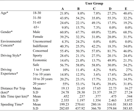
Table 1 presents a description of the participants contained within the five user groups in terms of their personal characteristics alongside a number of driving related attributes. This has been tabulated in order to determine the degree to which the groups are comparable in reference to their basic features. For all of the variables included in Table 1, appropriate hypothesis test have been employed to determine if the identified differences between groups are significant.

Reflecting on the results of these user group comparisons, it is evident that the groups used in this project display a number of visible differences from each other in terms of their personal characteristics and driving profiles. This has likely been generated as a result of the constrained nature of the project, which was unable to follow a strictly random sampling procedure. With this in mind, user group comparisons in the following analysis should be interpreted with caution. However, the user group differences identified in this study are unlikely to significantly affect how participant’s  behaviour  changed  over  time  meaning  that  temporal  variations  in  the  results, such as the degree to which a participant’s fuel consumption decreased, are  unlikely to be biased.

Table 1 Description of user groups employed in the project

User Group

A B C D E

Age* 18-30 21.8% 8.0% 7.8% 27.2% 48.6%

31-50 43.8% 54.2% 35.8% 55.3% 32.2%

51-65 24.6% 22.1% 49.1% 17.5% 19.2%

65+ 9.8% 15.7% 7.3% 0.0% 0.0%

Gender* Male 60.8% 67.7% 69.0% 72.0% 68.5%

Female 39.2% 32.3% 31.0% 28.0% 31.5%

Environmental Concern*

Unconcerned 4.3% 24.2% 0.0% 0.0% 0.0%

Indifferent 40.3% 25.5% 42.2% 18.3% 54.0% Concerned 55.4% 50.3% 57.8% 81.7% 46.0%

Driving Style* Sporty 28.6% 21.1% 27.5% 20.1% 24.4%

Economic 14.6% 21.0% 13.7% 49.9% 21.3%

Safe 56.7% 58.0% 58.8% 30.0% 54.2%

Driving Experience*

1 to 5 years 10% 11.4% 4.2% 9.6% 27%

5 to 10 years 14.8% 12.5% 3.6% 17.6% 26.6% 10 to 20 years 20.2% 23.1% 17.7% 33.2% 14.5%

20 years+ 55% 53.1% 74.4% 39.6% 31.8%

Distance Per Trip (km)*

Mean 19.13 21.65 17.65 22.73 16.27

S.D 24.78 28.30 21.57 38.27 27.24

Idle Time (per km)* Mean .452 .237 .377 .475 .544

S.D 2.355 1.197 1.354 2.463 3.872

Speeding Time* Mean 199.23 270.61 280.16 316.01 383.85

S.D 282.05 437.92 366.70 379.84 383.85

* Between group differences valid at the .000 level

3. Results and analysis

This section of the paper presents the analysis conducted on the data collected in the trial.

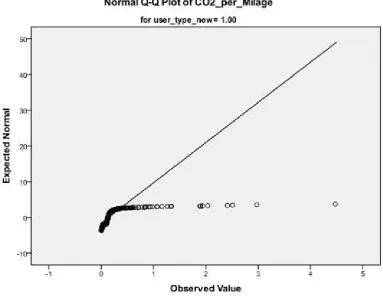
Initially the data was examined to determine whether or not it was normal or not to determine the best approach with regard to analysing data. Figure 3 indicates that the data is highly non-normal in distribution. As the data is non-normal in nature, a number of standard statistical test are no longer deemed valid. To overcome this problem, a number of non-parametric tests were conducted

Figure 3 Tests for normality

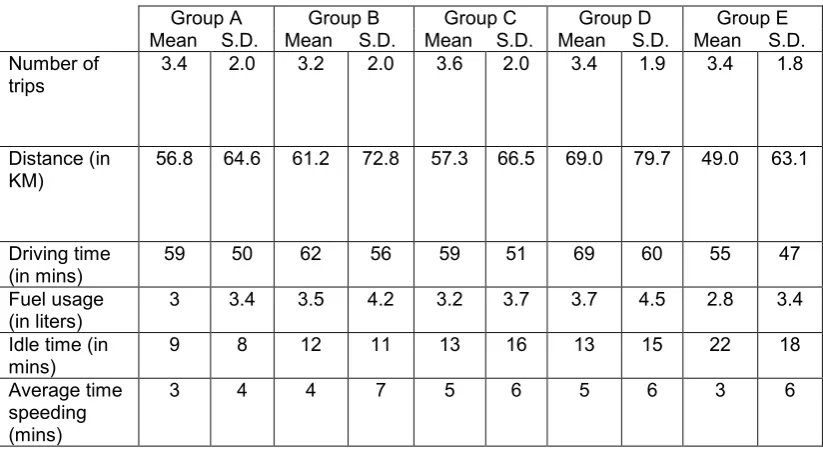
3.2 Descriptive Statistics

Table 2 Description of the data collected

Group A Group B Group C Group D Group E

Mean S.D. Mean S.D. Mean S.D. Mean S.D. Mean S.D. Number of

trips

3.4 2.0 3.2 2.0 3.6 2.0 3.4 1.9 3.4 1.8

Distance (in KM)

56.8 64.6 61.2 72.8 57.3 66.5 69.0 79.7 49.0 63.1

Driving time (in mins)

59 50 62 56 59 51 69 60 55 47

Fuel usage (in liters)

3 3.4 3.5 4.2 3.2 3.7 3.7 4.5 2.8 3.4

Idle time (in mins)

9 8 12 11 13 16 13 15 22 18

Average time speeding (mins)

3 4 4 7 5 6 5 6 3 6

3.3 Non Parametric Tests Between all Groups

For the purpose of analysis the primary metric under consideration is grams of carbon dioxide produced per kilometre driven. Table 3 displays the results of the non parametric test. Results of the Kruskal –Wallis test indicate that there are statistical differences between the observed means of the carbon dioxide emissions per kilometre, for the five experimental groups under examination.

Table 3: Non parametric test results between groups

Total N 22,231

Test Statistic 172.016

Degrees of freedom 4

Asymptotic Sig. (2 Sided test) .000

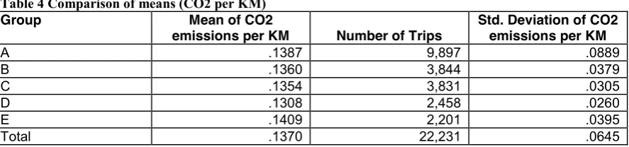
3.4 Emissions per group

Table 4 Comparison of means (CO2 per KM)

Group Mean of CO2

emissions per KM Number of Trips

Std. Deviation of CO2 emissions per KM

A .1387 9,897 .0889

B .1360 3,844 .0379

C .1354 3,831 .0305

D .1308 2,458 .0260

E .1409 2,201 .0395

Total .1370 22,231 .0645

As engines experience much greater emissions per km in the initial kilometres, due to the effects of start up emissions, it was decided to examine trips of varying distances. Table 5 presents all trips and their aver CO2 emissions per KM for trips 0-5 KM, 5-10 KM and all trips over 10KM. In all cases, as with unrestricted trips, the highest observed emissions are associated with the control group.

Table 5 Comparison of means (CO2 per KM) 0 – 5 KM in length

Group Mean of CO2

emissions per KM Number of Trips

Std. Deviation of CO2 emissions per KM

0-5KM trips

A .1336 9,778 .033

B .1347 3,820 .027

C .1347 3,812 .027

D .1303 2,445 .025

E .1398 2,190 .031

Total .1342 22,045 .030

5-10KM trips

A .1296 9,136 .025

B .1314 3,585 .022

C .1315 3,479 .023

D .1269 2,261 .019

E .1367 2,030 .027

Total .1307 20,491 .024

Trips over 10KM

A .1387 9,897 .089

B .1360 3,844 .038

C .1354 3,831 .031

D .1308 2,458 .026

E .1409 2,201 .040

Total .1370 22,231 .065

!

Table 6 Group C Emissions Reduction

User % Reduction

1 8.64

2 7.43

3 -12.10

4 10.88

5 10.26

6 14.56

7 2.15

8 10.34

9 27.49

Overall 8.85

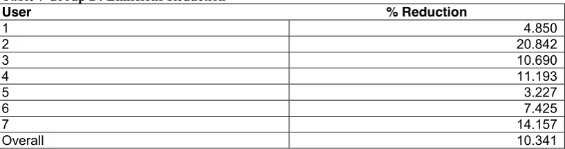
With regard to Group C average emissions reductions was observed to 8.85%, with the highest observed emissions reduction being 27.5%. The average emissions figure is somewhat skewed by participant number 3, who actually produced an emissions increase of 12%. If this participant is excluded from analysis the figure would be 11.2% Emission reductions for Group D were observed to be even lower than those observed for Group C, with an average emissions reduction of 10.3%.

Table 7 Group D: Emissions Reduction

User % Reduction

1 4.850

2 20.842

3 10.690

4 11.193

5 3.227

6 7.425

7 14.157

Overall 10.341

!

3.5 Emissions over the time period of the trial

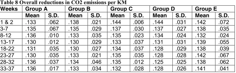
The following section reports the reductions in CO2 emissions from each of the five groups examined in the trial. In order to examine what if any reductions in CO2 occurred the emissions from the first two weeks of driving were averaged and used a baseline to compare subsequent weeks for reductions in emissions.

Table 8 Overall reductions in CO2 emissions per KM

Weeks Group A Group B Group C Group D Group E

Mean S.D. Mean S.D. Mean S.D. Mean S.D. Mean S.D.

1 & 2 .133 .062 .138 .021 .144 .006 .144 .031 .142 .072 3-7 .135 .067 .135 .029 .137 .030 .137 .027 .138 .035 8-12 .136 .010 .133 .035 .135 .023 .134 .024 .132 .024 13-17 .130 .012 .130 .029 .133 .037 .131 .031 .139 .055 18-22 .131 .035 .130 .027 .134 .037 .128 .029 .138 .039 23-27 .130 .035 .133 .021 .135 .035 .128 .028 .142 .067 28-32 .136 .037 .134 .046 .135 .012 .125 .025 .138 .062 33-37 .136 .017 .133 .034 .132 .028 .128 .026 .141 .041

In order to ascertain if drivers had different behavior on weekends compared to weekdays the dataset was divided between weekdays and weekends to determine if there was any difference. Table 9 presents the results for the weekends and Table 9 presents the results for weekdays. The findings for Group A shows that on average participants had higher average emissions on weekends. The results from Group B also show a similar trend with higher average emissions on weekends compared to weekdays. These trends are also shown for Groups C, D and E.

Table 9 Reductions in CO2 emissions - Weekends

Weeks Group A Group B Group C Group D Group E Mean S.D. Mean S.D. Mean S.D. Mean S.D. Mean S.D. 1 & 2 .134 .054 .142 .068 .135 .043 .162 .173 .136 .010 3-7 .138 .042 .143 .073 .147 .092 .142 .143 .147 .049 8-12 .137 .043 .139 .053 .129 .117 .137 .044 .135 .025 13-17 .135 .021 .133 .050 .139 .044 .130 .045 .138 .087 18-22 .137 .037 .129 .020 .139 .015 .129 .073 .144 .061 23-27 .137 .049 .129 .064 .139 .059 .128 .018 .150 .231 28-32 .138 .029 .138 .064 .133 .066 .126 .076 .138 .077 33-37 .136 .006 .140 .057 .131 .049 .130 .018 .146 .083

Table 10 Reductions in CO2 emissions - Weekdays

Weeks Group A Group B Group C Group D Group E

Mean S.D. Mean S.D. Mean S.D. Mean S.D. Mean S.D. 1 & 2 .119 .100 .134 .121 .134 .146 .133 .074 .143 .076 3-7 .133 .171 .135 .039 .137 .062 .138 .018 .136 .038 8-12 .136 .140 .132 .036 .136 .048 .138 .019 .131 .032 13-17 .125 .078 .129 .021 .132 .029 .132 .031 .138 .061 18-22 .123 .148 .124 .164 .134 .039 .127 .052 .137 .051 23-27 .120 .171 .120 .038 .134 .039 .128 .046 .138 .051 28-32 .136 .032 .136 .074 .134 .046 .125 .028 .136 .067 33-37 .135 .023 .139 .058 .132 .027 .127 .012 .139 .043

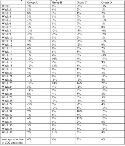
compared to the control group had higher average emissions per KM driven. The results in Table 10 show that on average each of the test groups had a greater reduction in CO2 emissions compared to the control sample. The results show that Group D performed the best with an average reduction in emissions of 6% compared to the control group. Groups A and B also had on average a 4% reduction in CO2 emissions compared to the control group with those in group C having a 3% decrease in emissions.

Table 11: Groups compared to control group

Group A Group B Group C Group D

Week 1 7% 1% -5% -3%

Week 2 8% 6% 2% 1%

Week 3 8% 3% 1% 2%

Week 4 3% 1% 0% 1%

Week 5 -7% 3% 2% -1%

Week 6 3% 1% 0% 1%

Week 7 3% 2% 0% 0%

Week 8 -3% -2% -5% -6%

Week 9 -2% -5% -2% -2%

Week 10 -12% 1% 2% 1%

Week 11 3% 4% -3% -1%

Week 12 0% 0% -2% 0%

Week 13 4% 6% 3% 2%

Week 14 7% 6% 8% 7%

Week 15 1% 4% 0% -3%

Week 16 12% 10% 6% 14%

Week 17 10% 7% 6% 9%

Week 18 12% 13% 3% 14%

Week 19 7% 6% 1% 7%

Week 20 4% 4% 3% 3%

Week 21 4% 6% 7% 11%

Week 22 -1% -1% -2% 4%

Week 23 18% 18% 14% 22%

Week 24 5% 4% -2% 11%

Week 25 14% 7% 8% 10%

Week 26 6% 4% 5% 8%

Week 27 2% 1% 0% 5%

Week 28 -7% -3% -4% 6%

Week 29 -3% 5% -2% 4%

Week 30 3% -2% 1% 10%

Week 31 7% 8% 10% 15%

Week 32 7% 8% 5% 14%

Week 33 6% 9% 13% 15%

Week 34 1% 1% 2% 6%

Week 35 5% 8% 6% 12%

Week 36 1% 0% 5% 11%

Week 37 7% 11% 6% 8%

Average reduction in CO2 emissions

4% 4% 3% 6%

3.6 Socio Economic Data

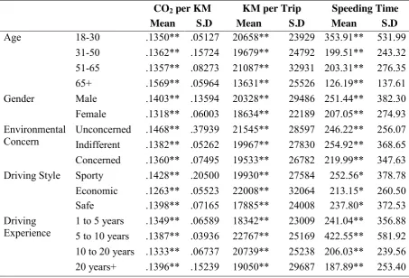
been conducted with the results presented in Table 12. The driving related variables which are explored in this analysis are CO2 emissions per kilometre, kilometres per

trip and the time spent speeding during a trip. Hypothesis testing has been utilised to determine if the differences identified are statistically significant. The results of these tests indicate that there is a substantial amount of variance identified, with all of the personal characteristics displaying significantly different averages for the driving related variables included.

In terms of CO2 emissions per kilometre, it is apparent that participants aged 65 years

and older emit significantly more compared to participants in the other age ranges and that male participants emit larger quantities compared to female participants. Participants who stated they are unconcerned about the environment tend to emit higher levels of CO2 compared to those participants who are concerned, whilst

participants who state they have a sporty driving style emit significantly higher CO2

levels than those who consider their driving to be economic. Whilst the difference observed in the CO2 emissions of participants of different levels of driving experience

is significant, there does not appear to be any substantial variation on this characteristic.

Shifting the focus to kilometres per trip, a number of interesting differences have been identified. Participants aged 65 years or older tend to drive significantly shorter distances, perhaps indicating that their car use is more orientated around local casual journeys. Female participants tend to have shorter trip lengths compared to males whilst participants who stated they are unconcerned about the environment have longer trip lengths than concerned participants. In reference to participant driving style, individuals who stated they drive in an economic manner have longer trip lengths compared to participants who state they drive in a safe manner whereas participants with the fewest years of driving experience tend to have shorter trip lengths.

Table 22 Socio-economic results from the sample

CO2 per KM KM per Trip Speeding Time

Mean S.D Mean S.D Mean S.D

Age 18-30 .1350** .05127 20658** 23929 353.91** 531.99 31-50 .1362** .15724 19679** 24792 199.51** 243.32 51-65 .1357** .08273 21087** 32931 203.31** 276.35 65+ .1569** .05964 13631** 25526 126.19** 137.61 Gender Male .1403** .13594 20328** 29486 251.44** 382.30 Female .1318** .06003 18634** 22189 207.05** 274.93 Environmental

Concern

Unconcerned .1468** .37939 21545** 28597 246.22** 256.07 Indifferent .1382** .05262 19967** 27830 254.92** 368.65 Concerned .1360** .07495 19533** 26782 219.99** 347.63 Driving Style Sporty .1428** .20500 19930** 27584 252.56* 378.78 Economic .1263** .05523 22008** 32064 213.15* 260.50 Safe .1398** .07165 17885** 24008 237.80* 372.53 Driving

Experience

1 to 5 years .1349** .06589 18342** 23009 241.04** 356.88 5 to 10 years .1387** .03936 22767** 25169 422.55** 581.92 10 to 20 years .1333** .06737 20739** 25238 206.03** 239.56 20 years+ .1396** .15239 19050** 29687 187.89** 253.40

* Between group differences valid at the .00 ** Between group differences valid at the .000

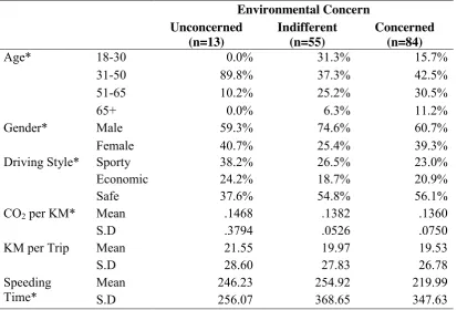
Table 13 Characteristics of project participants grouped by their stated level of environmental concern

Environmental Concern Unconcerned

(n=13)

Indifferent (n=55)

Concerned (n=84)

Age* 18-30 0.0% 31.3% 15.7%

31-50 89.8% 37.3% 42.5%

51-65 10.2% 25.2% 30.5%

65+ 0.0% 6.3% 11.2%

Gender* Male 59.3% 74.6% 60.7%

Female 40.7% 25.4% 39.3%

Driving Style* Sporty 38.2% 26.5% 23.0%

Economic 24.2% 18.7% 20.9%

Safe 37.6% 54.8% 56.1%

CO2 per KM* Mean .1468 .1382 .1360

S.D .3794 .0526 .0750

KM per Trip Mean 21.55 19.97 19.53

S.D 28.60 27.83 26.78

Speeding Time*

Mean 246.23 254.92 219.99

S.D 256.07 368.65 347.63

* Between group differences significant at the .000 level

Examining participants who stated they are unconcerned about the environment, this group tends to be populated by participants between the age of 30 and 50, with a somewhat even gender split whilst having a higher degree of individuals who either classify their driving style as sporty or economic. This finding might suggest that the desire of this group to drive in an economic manner is perhaps motivated by non-environmental issues, such as reducing vehicle operating costs. However, unconcerned participants also emit the highest quantity of CO2 emissions per

kilometer, which may indicate that the participants who are included in this group and specified a sporty driving style are more than compensating for those who stated an economic driving style.

For participants who stated they are indifferent towards the environment, this group displays a somewhat even spread over the first three age categories whilst containing a significantly higher number of males compared to the other two groups. In terms of driving style, indifferent participants hold a similar distribution to that of concerned drivers across the three options. Additionally, this participant group also tends to speed for longer periods compared to unconcerned and concerned drivers.

environmental concern. The safe driving tendencies of this group are further supported by the time spent speeding, with concerned participants having the lowest average across all three groups on this metric.

What this analysis demonstrates is that a single question which asks individuals to express their level of environmental concern proves to be an effective method of partitioning drivers into unique groups which display significant differences on a number of related characteristics. The identification of questions which allow for an effective partition of individuals might prove valuable in an attempt to find a working method which can reduce complex market segmentation solutions (Anable, 2005) into a much smaller number of key questions or variables.

4. Conclusions

An examination of the overall trend seen within the data would suggest that the provision of coaching could help to decrease emissions arising from driving. All experimental groups where some form of coaching was providing display lower emissions per kilometre values than the control group. An examination of the impact of introducing coaching to drivers was provided by Groups C and D, which received in car coaching and WEBFLEET, and WEBFLEET respectively. While both groups demonstrated decreased levels of emissions, it is not possible to ascertain whether the in car coaching significantly improved driver performance.

Acknowledgements

The authors would like to thank CURE and TomTom for their help with conducting and collecting the data for this trial. This work was sponsored by the European Commissions PEACOX Project under the Seventh Framework Programme (FP7).

References

Anable, J., 2005. “Complacent Car Addicts” or “Aspiring Environmentalists”?  Identifying travel behaviour segments using attitude theory. Transport Policy 12, 65– 78.

Barkenbus, J,. Eco-driving: An overlooked climate change initiative. Energy Policy 38, 2010, 762-769.

Beusen, B., Broekx, S., Denys, T., Beckx, C., Begraeuwe, B., Gijsbers, M., Scheepers, K., Govaerts, L., Torfs, R., Panis, L. Using on-board logging devices to study the longer-term impact of an eco-driving course. Transportation Research Part D. 14, 2009, 514-520.

Boriboonsomsin, K., Barth, M., Vu, A., Evaluation of driving behaviour and attitude towards eco-driving: A Southern California Limited Case Study. 90th Annual Meeting of the Transportation Research Board, Washington, D.C, January, 2011.

Martin, E., Boriboonsomisn, K., Chan, N., Williams, N., Shaheen, S., Barth, M. Dynamic ecodriving in Northern California: A Study of survey and vehicle operations data from an ecodriving feedback device. . 92nd Annual Meeting of the Transportation Research Board, Washington, D.C, January, 2013. Martin, E., Chan, N., Shaheen, S. Understanding how ecodriving public education

can result in reduced fuel use and greenhouse gas emissions. . 91st Annual Meeting of the Transportation Research Board, Washington, D.C, January, 2012.

Stillwater, T., Kurani, K. In-vehicle ecodriving interface: Theory, design and driver responses. 91st Annual Meeting of the Transportation Research Board, Washington, D.C, January, 2012.

Rutty, M., Matthews, L., Andrey, J., Del Matto, T. Eco-driver training within the City  of  Calgary’s  municipal  fleet:  Monitoring  the  impact.    Transportation  Research Part D. 24, 2013, 44-51.