Source and sink carbon dynamics and carbon allocation in the Amazon basin

Source and sink carbon dynamics and carbon

allocation in the Amazon basin

Christopher E. Doughty1, D. B. Metcalfe2, C. A. J. Girardin1, F. F. Amezquita3, L. Durand3, W. Huaraca Huasco3, J. E. Silva-Espejo3, A. Araujo-Murakami4, M. C. da Costa5, A. C. L. da Costa5, W. Rocha6, P. Meir7,8, D. Galbraith9, and Y. Malhi1

1

Environmental Change Institute, School of Geography and the Environment, University of Oxford, Oxford, UK,2Department of Physical Geography and Ecosystem Science, Lund University, Lund, Sweden,3_{Universidad Nacional San Antonio Abad del}

Cusco, Cusco, Peru,4Museo de Historia Natural Noel Kempff Mercado, Universidad Autónoma Gabriel René Moreno, Santa Cruz, Bolivia,5_{Instituto de Geociências, Universidade Federal do Pará, Belém, Brazil,}6_{Amazon Environmental Research Institute,}

Canarana, Brazil,7School of Geosciences, University of Edinburgh, Edinburgh, UK,8Research School of Biology, Australian National University, Canberra, ACT, Australia,9_{School of Geography, University of Leeds, Leeds, UK}

Abstract

Changes to the carbon cycle in tropical forests could affect global climate, but predicting such changes has been previously limited by lack offield-based data. Here we show seasonal cycles of the complete carbon cycle for 14, 1 ha intensive carbon cycling plots which we separate into three regions: humid lowland, highlands, and dry lowlands. Our data highlight three trends: (1) there is differing seasonality of total net primary productivity (NPP) with the highlands and dry lowlands peaking in the dry season and the humid lowland sites peaking in the wet season, (2) seasonal reductions in wood NPP are not driven by reductions in total NPP but by carbon during the dry season being preferentially allocated toward either roots or canopy NPP, and (3) there is a temporal decoupling between total photosynthesis and total carbon usage (plant carbon expenditure). This decoupling indicates the presence of nonstructural carbohydrates which may allow growth and carbon to be allocated when it is most ecologically beneficial rather than when it is most environmentally available.

1. Introduction

The net carbon fluxes in tropical forests have profound consequences for global climate, and there is uncertainty on how they are going to change under drought and climate change [Cox et al., 2013; Doughty et al., 2015;Friedlingstein et al., 2006;Meir et al., 2008], but we lack accuratefield data with which to test models that predict these consequences. Comparisons of spatial and temporal variations of aboveground measured net primary production (NPP) do not currently show close correlations with either modeled or remotely sensed NPP [Cleveland et al., 2015]. Currently, the few field observations of NPP that exist are composed mainly of aboveground NPP (litterfall and wood NPP) which are often estimated on an annual basis and extrapolated to estimate total NPP [Chave et al., 2010; Phillips et al., 1998]. However, a decrease in aboveground NPP may reflect a shift in allocation toward belowground

fine root production [Doughty et al., 2014b; Metcalfe et al., 2010b] rather than a decline in total NPP. Therefore, it is valuable to quantify all components of NPP in an ecosystem, especiallyfine root production (because it is so rarely collected).

Eddy covariance measurements can be used to estimate seasonal cycles in total photosynthesis by adding seasonal cycles in nighttime respiration to seasonal cycles in net ecosystem exchange (NEE) [Baldocchi, 2003]. However, eddy covariance towers are difficult and expensive to install in tropical forests, and adverse meteorological conditions, such as lack of nighttime turbulence, can constrain accuracy [Miller et al., 2004]. More fundamentally, eddy covariance can quantify only the net carbon flux between ecosystem and the atmosphere and cannot easily partition this flux into component processes. Eddy covariance measurements can be used to estimate the seasonality of total photosynthesis or gross primary production (GPP), and GPP estimates have shown increases toward the end of the dry season in the eastern Amazon [Doughty and Goulden, 2008;Saleska et al., 2003]. This increase may be because eastern Amazon leaves flush in the dry season, taking advantage of the increased irradiance during this period [Vanschaik et al., 1993], and because new leaves tend to fix carbon more efficiently, this increases total canopy photosynthesis [Doughty and Goulden, 2008].

Global Biogeochemical Cycles

RESEARCH ARTICLE

10.1002/2014GB005028

Special Section:

Trends and Determinants of the Amazon Rainforests in a Changing World, A Carbon Cycle Perspective

Key Points:

•Total tropical forest NPP peaks in the wet season in the humid lowlands

•Seasonal reductions in wood NPP are not driven by reductions in total NPP

•There is a temporal decoupling between GPP and carbon usage

Supporting Information:

•Text S1, Figures S1–S8, and Tables S1–S4

Correspondence to: C. E. Doughty,

[email protected]

Citation:

Doughty, C. E., et al. (2015), Source and sink carbon dynamics and carbon allocation in the Amazon basin,Global Biogeochem. Cycles,29, 645–655, doi:10.1002/2014GB005028.

Received 28 OCT 2014 Accepted 22 APR 2015

Accepted article online 23 APR 2015 Published online 25 MAY 2015

To accurately model long-term woody biomass in the tropics, GPP is only part of the story. It is important to know the percentage of total photosynthesis that goes toward growth and the percentage of total growth that goes toward wood biomass [Malhi et al., 2011]. Total autotrophic respiration plus total NPP (equal to plant carbon expenditure (PCE)) should approximately equal total GPP over long time scales and at equilibrium. However, over shorter time scales, the two may differ as forests may store carbon and only use it when it is ecologically beneficial. This carbon may be stored in the form of nonstructural carbohydrates (NSCs—long-term energy storage in the form of starch, sucrose, and hexose sugars), which may be abundant in tropical forests [Newell et al., 2002;Poorter and Kitajima, 2007;Wurth et al., 2005].

There is increasing interest in NSCs and recognition of their potential important role in tropical forests. Storage of NSCs has not been quantified often, and its role in drought responses remains unclear [Meir et al., 2015], but it may be a missing piece of the puzzle explaining seasonality of growth and potential mismatches between GPP and growth if C is stored at one point and used later. One study measured total NSC pools (wood, leaves, and roots) in a tropical forest in Panama and found that there was more than sufficient stored carbon to reflush the entire canopy [Wurth et al., 2005]. In temperate forests, one study found NSCs to be highly dynamic with concentrations of sugars and starches 2–4 times greater in the growing season than the dormant season and a mean age of the starches and sugars of about a decade based on radiocarbon dating [Richardson et al., 2013]. In an aspen stand, NSCs were an important store of carbon (15–20% of dry mass in root tissues) but did not decrease during a drought period, and therefore, the authors attributed drought-related death in aspen to hydraulic failure rather than carbon starvation [Anderegg et al., 2012]. In tropical forests, these NSCs have not been accounted for in most studies and could play a role in aiding tropical forests through drought [Doughty et al., 2015, 2014b;Meir et al., 2015]. Seasonal carbon storage in tropical forests can also be estimated by comparing “source”versus “sink” carbon, which in practice would compare eddy covariance-calculated GPP versus bottom-up derived plant carbon expenditure (PCE, the amount of carbon used for NPP andRa) [Doughty et al., 2014a;Malhi et al.,

2009;Metcalfe et al., 2010a;Palacio et al., 2014].

Recently, there have been descriptions of seasonality in aboveground NPP [Chave et al., 2010;Phillips et al., 1998], and seasonality in photosynthesis across a network of tropical forest eddy covariance towers [Restrepo-Coupe et al., 2013], but to the best of our knowledge, there are no continental scale studies of the seasonality in total NPP,Ra, and PCE in tropical forests. In recent years, we have developed a network of intensive monitoring

plots in tropical forests across Amazonia and presented site-specific descriptions of the seasonality of the components of NPP andRa[Araujo-Murakami et al., 2014;da Costa et al., 2014;del Aguila-Pasquel et al., 2014;

Doughty et al., 2014a;Girardin et al., 2014; Huasco et al., 2014;Malhi et al., 2014; Rocha et al., 2014]. In this study, we aggregate these data and show seasonal patterns of NPP, autotrophic respiration (Ra), carbon

allocation (allocation of NPP to a specific organ such as wood leaves orfine roots divided by total NPP), and plant carbon expenditure (PCE—total NPP plusRa) from 14, 1 ha plots across Amazonia that were measured

over a 2–3 year period. We then compare PCE to an estimate of total photosynthesis (GPP) as calculated using eddy covariance measurements (net ecosystem exchange minus average nighttime respiration) and a vegetation model (Joint UK Land Environment Simulator (JULES)). We test the following hypotheses:

1. Total NPP, autotrophic respiration, and PCE will have different seasonal cycles in three distinct regions of tropical forest (humid lowland, highland, and dry lowlands).

2. Allocation of carbon will vary seasonally in different biomass components over a seasonal cycle. 3. Sink or carbon usage (NPP + respiration) will not have the same seasonal pattern as source or top-down

GPP (eddy covariance or modeled GPP) over a seasonal cycle.

2. Methods

lowlands, has shallow soils and species typical of a dry deciduous forest. The other plot, which we classify as lowland humid tropical, has deep soils and species typical of the humid Amazon. For further clarity, we show the data plotted separately for each plot for all carbon and allocation terms in Figures S1–S3 and S5–S7 in the supporting information.

[image:3.612.172.574.92.344.2]

We measured total NPP and autotrophic respiration from mainly 2009 to 2011 (see Tables S1 and S2 in the supporting information for details) with most methodological details in the supporting information. Total NPP consists offine root NPP measured with ingrowth cores, wood NPP measured with dendrometers and annual censuses, and canopy NPP which quantifies leafflush by summing the monthly change in leaf area index (LAI) multiplied by site-specific specific leaf area and litter fall [Doughty and Goulden, 2008]. In our seasonal estimates of NPP, we exclude several smaller components such as branch fall, herbivory, coarse root, and small tree NPP (<10 cm) that we have included in previous annual budgets of these sites, focussing instead on the seasonality of the three major components of NPP. We estimate that these smaller terms account for ~20% of total NPP. Total autotrophic respiration consists of rhizosphere respiration determined with a soil partitioning experiment and an infrared gas analyzer (EGM-4, PP systems, Amesbury, USA), wood respiration measured using an EGM-4, and scaled to the canopy by multiplying by the plot’s woody surface area and canopy respiration measured using measured LAI and a CIRAS-2 leaf gas exchange system (PP systems, Amesbury, USA). Each component was measured every 1–3 months, except for canopy respiration which was measured only 1–2 times per plot at the leaf level, and in the case of one site (Cax), estimated from earlier single time-point measurements. We estimate total plant carbon expenditure (PCE) as the summation of total NPP and total autotrophic respiration, and it is equal to gross primary production (GPP) on longer time scales (>1 year). Detailed information on the methodology and graphs showing data from each individual carbon cycling component are available in the in the supporting information and from a series of companion papers [Araujo-Murakami et al., 2014; da Costa et al., 2014;del Aguila-Pasquel et al., 2014;Doughty et al., 2014a;Girardin et al., 2014;Huasco et al., 2014;Malhi et al., 2014;Rocha et al., 2014]. The methods are also described in detail in the online manual of the Global Ecosystems Monitoring (GEM) network (www.gem.tropicalforests.ox.ac.uk).

For each region (humid lowland, highland, and dry lowlands), we average each carbon cycle component (total NPP, autotrophic respiration, and PCE) over a 2–3 year period (2009–2011) for each month. All error bars shown in this paper are spatial errors of differences among plots (but in our companion papers, for each measurement, we provide estimates of both sampling error associated with spatial variation in the variables measured and measurement uncertainty regarding scaling localized measurements to whole-tree and whole-plot estimates). The trends across sites are reasonably consistent, and this provides some confirmation that the effects are real, but it does not eliminate the possibility that measurement artifacts across all sites are responsible for the purported effects. If there were any data gaps, wefilled them using data from a similar monthly period. There was only one instance where an entire class of data was not collected. We did not collect leaf respiration from one of the Brazilian dry lowland sites (Tanguro), and we therefore took available data from the nearby dry lowland site that had similar climate in Bolivia (Kenia) [Araujo-Murakami et al., 2014;Rocha et al., 2014].

Meteorological data were provided by eight automatic weather stations, one at each plot, which measure solar radiation (W m2), precipitation (mm mol1), air temperature (°C), and humidity (%) (Skye Instruments, Llandrindod, UK). Individual site-specific meteorological data are available in the companion papers. Statistical analysis was done using a pairedttest, pairing wet and dry season means for each year (May to October dry season versus November to April wet season) and each region (highland–N= 8 (four plots × 2 years), dry lowland–N= 9 (three plots × 3 years), and lowland–N= 14 (seven plots × 2 years)). Difference among regions was done using a one-way repeated measures analysis of variance (ANOVA). If the data did not meet the normality tests, we used the Kruskal-Wallis one-way analysis of variance on ranks, and medians were used instead of means. To calculate percent carbon allocation, we take each individual component (wood, canopy, andfine roots) and divide by the sum of these components of NPP (wood, canopy, andfine roots).

To partition how much of the seasonal variation in wood growth was caused by a shift in NPP allocation between seasons versus a shift in total NPP, we employed the following equation (results for each section of the equation shown in the last three columns of Table 1):

Wdry Wwet¼

αdry αwet*

Ndry

Nwet (1)

whereWis the wood production,αis the fraction of total NPP allocated to wood, andNis the total NPP. Thefirst term on the right represents the shift in NPP allocation to wood between dry and wet seasons and the second term represents the shift in total NPP between seasons. The whole expression is a mathematical identity and simply facilitates the partitioning of the relative importance of total NPP versus NPP allocation in determining seasonal shifts in wood production.

[image:4.612.49.573.138.196.2]

To estimate the effect of moisture expansion (of bark or xylem) on apparent tree growth during the wet season at the plot level, we separated the trees with almost no annual tree growth (woody NPP<1 kg C ha1yr1) and determined their apparent seasonal trends in diameter. For these slow growing trees, we found a mean seasonal amplitude of apparent growth peaking in April and then decreasing until October. For example, the mean estimated seasonal correction for all plots (Table S3 in the supporting information) for moisture expansion between March and November (the maximum and minimum) to be 0.04 Mg C ha1month1(see Table S3 in the supporting information for the results for all sites). We note that this approach may underestimate the moisture expansion effect because faster growing trees tend to shrink more in the dry

Table 1. Average Annual Values for Seven Humid Lowland Sites (Four in Caxiuanã, Two in Tambopata, and One in Kenia-Wet, Bolivia), Highland (Two in San Pedro, Peru and Two in Wayquecha, Peru), and Dry Lowlands (Two in Tanguro and One in Kenia-Dry, Bolivia) for GPP, NPP, Carbon Use Efficiency (CUE), Percentage Carbon Allocated to Canopy, Wood and Fine Roots, and the Percentage Ratio of Wood NPP, Wood Allocation, and Total NPP in the Dry Season Compared Relative to the Wet Season

GPP Mg C ha1yr1 NPP Mg C ha1yr1 CUE (%) % Canopy % Wood % Fine

Root

Ratio d/w Wood NPP

Ratio d/w Wood Allocation

season because they possess larger vessels. While it would be desirable, we had inadequate data to correct for moisture expansion at the detailed level of species or by tree girth.

We estimate GPP at two of the sites with two methods: (1) using data from the vegetation model Joint UK Land Environment Simulator (JULES) vegetation model [Best et al., 2011; Clark et al., 2011] parameterized for Tambopata and (2) using data from an eddy covariance tower in Caxiuanã, Brazil, over the period of 1999– 2002 [Carswell et al., 2002]. We assume that over a yearly period, total GPP from photosynthesis will approximately equal total carbon expended by NPP and autotrophic respiration (NPP +Ra= PCE). We

therefore normalize the GPP for comparison to the bottom-up estimates. JULES is closely based on the Met Office Surface Energy Scheme–Terrestrial Representation of Interactive Foliage and Flora Including Dynamics land surface scheme and was forced with high-resolution Princeton meteorological forcing, which was extracted for the grid cells (1° × 1°) corresponding to the plots [Sheffield et al., 2006]. Simulations were spun-up from bare ground to equilibrium under preindustrial CO2 (278 ppm) using the cycled meteorological drivers. From the equilibrium state, CO2was increased following observed atmospheric CO2concentrations. Soil texture and depth used in each simulation were based on in situ data. One of our ground-based plots was within the footprint of an eddy covariance tower at Caxiuanã, Para, Brazil [Carswell et al., 2002], and therefore, we compare PCE at our four, 1 ha Caxiuanã plots to light saturated net ecosystem exchange (NEE) plus nighttime respiration to estimate GPP. We use gap-filled NEE data over 3 years (1999 to 2002) subtracting average monthly nighttime respiration to calculate monthly GPP. More recent data from this tower were not available for comparison, but we assume no major differences in vegetation structure or density between the different periods. To estimate percentage monthly incoming carbon, we took monthly GPP and divided by summed annual GPP. For further details on the processing of these data, seeCarswell et al. [2002] andRestrepo-Coupe et al. [2013] [Carswell et al., 2002;Restrepo-Coupe et al., 2013].

3. Results

3.1. Meteorology and Average Site Differences

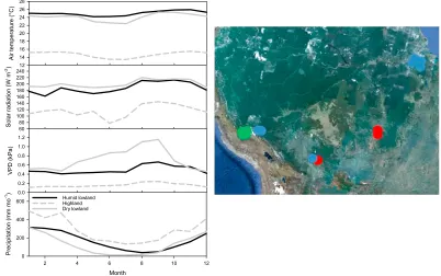
Although tropical forests are not noted for the seasonality in climate compared with other regions, each of our three regions did show aspects of seasonality in climate (Figure 1). In our lowland humid plots, there is seasonality in precipitation which is reduced in the months of June to August with a concurrent increase in solar radiation. In the lowland dry forest plots, there is high VPD and low precipitation from April to August. In the highland regions on the Andean slope, there is generally very low VPD, high precipitation, and overall low sun conditions associated with cloudiness, but solar irradiance increases from June to September. Climate trends for individual plots can be viewed in the companion papers listed in the methods.

We find clear differences in annually averaged GPP and NPP among the three regions (humid lowland, highland, and dry lowland) (Table 1). GPP is the highest at the humid lowland sites, followed by the highlands (although we note in companion papers the large difference in GPP between the 3000 m and the 1500 m sites and differences in estimates at high elevation and the dry lowlands). NPP, and by proxy carbon use efficiency (CUE), shows different trends. The highlands have the lowest NPP and CUE followed by the dry lowland and the humid lowlands. The dry lowland and the highland plots allocate their carbon, on average in very similar ways, with a larger share toward leaves compared to lowland humid plots. The lowland humid plots differ by allocating less carbon on average toward leaves and instead more towardfine roots.

3.2. Seasonality of NPP, Autotrophic Respiration, and PCE

seasonality in NPP to the humid lowland plots, but the third plot shows a seasonality that is inverse to the other two (Figure S1 in the supporting information).

There is likewise seasonality in autotrophic respiration at each of the sites, with the lowest autotrophic respiration between May and September when both total NPP and temperatures are at a minimum (Figure 2b). Total seasonality is smaller in autotrophic respiration than NPP at the humid lowland site with a difference of only 12% between the maximum and minimum monthly values. In the humid lowland sites, there is no overall significant seasonality (P>0.05, N= 14), and it is split, with the four Caxiuanã plots showing limited seasonality in autotrophic respiration and the Peruvian and Bolivian sites showing stronger seasonality (Figure S2 in the supporting information). Seasonality in autotrophic respiration at the highland (highly significant—P<0.005) and lowland dry sites vary (highly significant—P<0.005), with a difference of 22 and 24% between the maximum and minimum monthly values, respectively.

[image:6.612.219.531.92.419.2]

We add the total autotrophic respiration to the total NPP over a seasonal cycle to get an estimate of PCE (Figure 2, bottom). Humid lowland PCE displays the lowest seasonality but still significant (P<0.05,N= 14) with a 15% difference between the maximum and minimum months. The highlands (significant—P<0.05, N= 8) and dry lowland plots (highly significant—P<0.01,N= 9) show a similar seasonality, with 21–25% variability. At most sites, the minimum PCE is between ~June and July. Total PCE is dominated by autotrophic respiration, and the trends broadly match those of autotrophic respiration seasonality. The timing of peaks in PCE also vary across sites, with the highlands peaking in September, the dry lowland plots peaking in November, and the lowland humid plots peaking in January. There was variation in the

seasonality of PCE in the lowland sites mainly among the Caxiuanã sites and the other plots and in the highland plots between the midelevation (~1500 m) and the high-elevation plots (~3000 m) (Figure S3 in the supporting information). Our ANOVA results indicate that there were significant P<0.05 differences among all sites in mean PCE, NPP, andR_awhen separated for the wet and dry season values (Table S4 in the supporting information).

3.3. Carbon Allocation

[image:7.612.219.529.90.417.2]

Carbon allocation also shows strong seasonality in each region (Figure 3) with peaks in canopy allocation between July and November (dry season) across all sites. Our ANOVA results indicate there were significantP<0.05 differences in median wet and dry seasonal values among sites for wood andfine roots but not for canopy (P>0.05) (Table S4 in the supporting information). The canopy fraction of NPP, at the peak, accounts for 47% of lowland humid plot NPP, 68% of highland plot NPP, and 74% of dry lowland plot NPP. In contrast, at all sites,fine root allocation peaked in the December to January period (wet season) with allocation towardfine root growth at the peak 48% in the humid lowlands, 35% in the highland plots, and 26% in the dry lowland plots. Wood NPP allocation decreased during the dry season when leafflush was most prevalent. Allocation to wood NPP allocation peaked at 30% in the humid lowlands, 44% in the highlands, and 35% in the dry lowlands. Carbon allocation patterns varied more strongly among plots in the dry lowlands and highlands than the humid lowland plots (Figures S5–S7 in the supporting information). At the lowland humid plots, the dry season NPP was 76 ± 11% of wet season NPP, and dry season allocation to wood was only 66 ± 12% of wet season allocation; these two factors combined to result in dry season wood NPP being 51 ± 10% of wet season NPP (Table 1 and equation (1)). Therefore, allocation changes are slightly more important than changes in NPP in driving seasonality of wood growth. Allocation was more important

in the dry lowlands, with dry season NPP 76 ± 19% of wet season NPP, and dry season allocation to wood only 34 ± 20% of wet season allocation; these two factors combined to result in dry season wood NPP being 26 ± 19% of wet season NPP and allocation more than twice as important as changes in total NPP. There was little average seasonality in wood NPP at the highland site because seasonality in allocation appears to offset seasonality in NPP.

3.4. PCE Versus Photosynthesis

We compare the seasonality of PCE to GPP estimates obtained from eddy covariance measurements at Caxiuanã and from modeled GPP estimates for Tambopata (Figure 4). In the dry season, JULES predicts a decrease in photosynthesis, but the observations show that carbon usage during this period remains fairly high. This suggests a potential role for NSC to sustain high growth rates during the dry season in these forests. During the dry season, estimated carbon use (PCE) is greater than estimated total photosynthesis suggesting that the additional carbon must come from stored carbohydrate, presumably NSC. In the wet season, carbon used is less than total photosynthesis, suggesting that it is stored during these periods. We also compare total carbon used at the Caxiuanã sites to total photosynthesis as measured by an eddy covariance tower, from within the same region of Brazil (Figure 4b). We see slightly different seasonal patterns but a similar message that total photosynthesis does not appear to match total carbon used on a seasonal basis. This is not due to different weather patterns between the two study periods because the seasonality of weather in our plots is the same as that at the tower site (Figure S8 in the supporting information).

4. Discussion

[image:8.612.217.532.93.318.2]

Our data highlight three trends: (1) there is differing seasonality of total NPP with more carbon-limited sites (highland and dry lowlands) peaking in the dry/sunny season and lowland humid sites peaking in the wet season and (2) wood NPP (stem growth) decreases in the dry season in lowland humid and dry lowland plots. This shift is more caused by seasonality in allocation rather than seasonality in NPP, particularly in the dry lowland plots, and (3) at the sites we are able to compare withflux tower or model data, there is some evidence of a temporal decoupling between total photosynthesis and total carbon usage. This result suggests the important role that sugar pools such as NSC may play in tropical forests, with plants able to draw in NSC reserves to maintain NPP in the dry season [Richardson et al., 2013;Wurth et al., 2005].

The difference in seasonality of NPP may be related to the carbon dynamics of the plots. For instance, annual mean carbon allocation toward leaves is greater at the highland and dry lowlands plots than the humid lowland plots (~50% versus ~40%). Total GPP is also lower at the highland and dry lowlands plots than the humid lowland plots (30 versus 36 Mg C ha1yr1%) [Araujo-Murakami et al., 2014;Doughty et al., 2014a; Girardin et al., 2014]. This indicates that the carbon assimilation in highland and dry forest sites may be limited by either water (dry lowlands) or temperature and light constraints (highlands) [Bloom et al., 1985; van de Weg et al., 2014]. July through October is when solar radiation at all sites begins to peak, and September is also a peak in NPP in all three regions. Therefore, the humid lowlands, which appear less carbon limited, can continue peak growth beyond the sunniest conditions and into the cloudier wet season. However, reduced carbon uptake during the cloudier wet season may reduce carbon uptake sufficiently to cause the more carbon-limited dry and highland sites to minimize growth (Figure 2). Seasonality in both autotrophic respiration and PCE was less than seasonality in NPP in all regions; however, the seasonal differences are reduced when canopy respiration is removed (35% versus 41–50%) (Figure S4 in the supporting information). Autotrophic respiration can be described as a function of aQ₁₀temperature dependency of maintenance respiration combined with the metabolic costs of growth [Amthor, 2000; Cannell and Thornley, 2000]. Both growth and temperature have a minimum near May and June, and we also see a reduction in autotrophic respiration at this point. Therefore, as expected, our data lend some support to the notion that seasonality in autotrophic respiration is correlated to both temperature and total growth rates.

Our data showed strong seasonal differences in allocation at all plots. More specifically, allocation toward leaves was highest during periods when incoming solar irradiance is maximized, and allocation toward wood andfine roots was higher during other periods of the year. This trade-off appears dominant at all three regions of interest. This is interesting because traditionally, it has been thought that wood growth slows during the dry season primarily in response to reduced photosynthesis under drier conditions [Brienen and Zuidema, 2005; Phillips et al., 1998], but our data suggest that at the humid lowland sites, allocation is slightly more important and more than twice as important as growth in the dry sites for controlling seasonality of wood NPP. Why does leaf production peak in the dry/sunny season? It may be a direct abiotic optimization to build new, high photosynthetic capacity leaf material when light availability is highest or it may be the result of biotic pressures with reduced pathogen or fungus load in dry season conditions, making the dry season an optimum time to produce young, unprotected leaves [Givnish, 1999].

For the sites we examined, seasonality in total photosynthesis does not match seasonality in PCE (Figure 4), although large error bars in our data add caution to our interpretation. Sugars arefixed by photosynthesis when conditions are favorable for photosynthesis, and they are then transported throughout the tree through the phloem [Kuptz et al., 2011]. Previous studies have found that these sugar stores in a forest in Panama are roughly 16 Mg C ha1, which is more than enough carbon to refoliate an entire canopy [Wurth et al., 2005]. There are seasonal differences in NSC concentrations, and previous studies of NSCs in tropical forest seedlings found that a fourfold difference between dry season maxima and wet season minima in branch wood tissue [Newell et al., 2002]. There are also differences in NSCs between moist and dry forests with moist forest species having higher NSC concentrations than dry forest species [Poorter and Kitajima, 2007]. However, more data are still needed to test for generality of these trends in other tropical forests, especially for total NPP. Seasonality patterns in NPP appear instead driven by when it is most advantageous for the tree to invest in a particular organ. For instance, irradiance increases between April and August in much of the humid lowland tropics and trees appear to invest carbon in

flushing new leaves. Later in the year, they invest in wood and roots, presumably to gain height and acquire soil resources.

steady despite decreased photosynthesis [Doughty et al., 2015, 2014b], and therefore, NSCs must allow growth to continue during the drought period. However, with severe enough drought, mortality will occur, possibly when all available NSCs are utilized [Meir et al., 2015; Metcalfe et al., 2010b; P. Meir et al., Threshold responses to soil moisture deficit by trees and soil in tropical rain forests: Insights from field experiments, submitted toBioScience, 2015]. Therefore, the quantity of NSC contained in forests may hold the key to resilience to drought and it must be better quantified in future studies. Having a better estimate of this number may allow us to better predict how resilient tropical forests will be to future climate changes.

References

Amthor, J. S. (2000), The McCree-de Wit-Penning de Vries-Thornley respiration paradigms: 30 years later,Ann. Bot. London,86(1), 1–20. Anderegg, W. R. L., J. A. Berry, D. D. Smith, J. S. Sperry, L. D. L. Anderegg, and C. B. Field (2012), The roles of hydraulic and carbon stress in a

widespread climate-induced forest die-off,Proc. Natl. Acad. Sci. U.S.A.,109(1), 233–237.

Araujo-Murakami, A., et al. (2014), The productivity, allocation and cycling of carbon in forests at the dry margin of the Amazon forest in Bolivia,Plant Ecol. Divers.,7(1–2), 55–69.

Baldocchi, D. D. (2003), Assessing the eddy covariance technique for evaluating carbon dioxide exchange rates of ecosystems: Past, present and future,Global Change Biol.,9(4), 479–492.

Best, M. J., et al. (2011), The Joint UK Land Environment Simulator (JULES), model description—Part 1: Energy and waterfluxes,Geosci. Model Dev.,4(3), 677–699.

Bloom, A. J., F. S. Chapin, and H. A. Mooney (1985), Resource limitation in plants—An economic analogy,Annu. Rev. Ecol. Syst.,16, 363–392. Brienen, R. J. W., and P. A. Zuidema (2005), Relating tree growth to rainfall in Bolivian rain forests: A test for six species using tree ring analysis,

Oecologia,146(1), 1–12.

Cannell, M. G. R., and J. H. M. Thornley (2000), Modelling the components of plant respiration: Some guiding principles,Ann. Bot. London, 85(1), 45–54.

Carswell, F. E., et al. (2002), Seasonality in CO2and H2Oflux at an eastern Amazonian rain forest,J. Geophys. Res.,107(D20), 43-1–43-16, doi:10.1029/2000JD000284.

Chave, J., et al. (2010), Regional and seasonal patterns of litterfall in tropical South America,Biogeosciences,7(1), 43–55, doi:10.5194/bg-7-43-2010. Clark, D. B., et al. (2011), The Joint UK Land Environment Simulator (JULES), model description—Part 2: Carbonfluxes and vegetation

dynamics,Geosci. Model Dev.,4(3), 701–722, doi:10.5194/gmd-4-701-2011.

Cleveland, C. C., P. Taylor, K. D. Chadwick, K. Dahlin, C. E. Doughty, Y. Malhi, W. K. Smith, B. W. Sullivan, W. R. Wieder, and A. R. Townsend (2015), A comparison of plot-based, satellite and Earth system model estimates of tropical forest net primary production,Global Biochem. Cycles, 29, doi:10.1002/2014GB005022.

Cox, P. M., D. Pearson, B. B. Booth, P. Friedlingstein, C. Huntingford, C. D. Jones, and C. M. Luke (2013), Sensitivity of tropical carbon to climate change constrained by carbon dioxide variability,Nature,494(7437), 341–344, doi:10.1038/nature11882.

da Costa, A. C. L., et al. (2014), Ecosystem respiration and net primary productivity after 8–10 years of experimental through-fall reduction in an eastern Amazon forest,Plant Ecol. Divers.,7(1–2), 7–24, doi:10.1080/17550874.2013.798366.

del Aguila-Pasquel, J., et al. (2014), The seasonal cycle of productivity, metabolism and carbon dynamics in a wet aseasonal forest in north-west Amazonia (Iquitos, Peru),Plant Ecol. Divers.,7(1–2), 71–83, doi:10.1080/17550874.2013.798365.

Doughty, C. E., and M. L. Goulden (2008), Seasonal patterns of tropical forest leaf area index and CO2exchange,J. Geophys. Res.,113, G00B06, doi:10.1029/2007JG000590.

Doughty, C. E., et al. (2014a), The production, allocation and cycling of carbon in a forest on fertile terra preta soil in eastern Amazonia compared with a forest on adjacent infertile soil,Plant Ecol. Divers.,7(1–2), 41–53, doi:10.1080/17550874.2013.798367.

Doughty, C. E., et al. (2014b), Allocation trade-offs dominate the response of tropical forest growth to seasonal and interannual drought, Ecology,95(8), 2192–2201, doi:10.1890/13-1507.1.

Doughty, C. E., D. B. Metcalfe, C. A. J. Girardin, K. Halladay, A. C. L. da Costa, and Y. Malhi (2015), Drought impact on forest carbon dynamics andfluxes in Amazonia,Nature,519, 78–82, doi:10.1038/nature14213.

Friedlingstein, P., et al. (2006), Climate-carbon cycle feedback analysis: Results from the (CMIP)-M-4 model intercomparison,J. Clim.,19(14), 3337–3353, doi:10.1175/JCLI3800.1.

Girardin, C. A. J., et al. (2014), Productivity and carbon allocation in a tropical montane cloud forest in the Peruvian Andes,Plant Ecol. Divers., 7(1–2), 107–123, doi:10.1080/17550874.2013.820222.

Givnish, T. J. (1999), On the causes of gradients in tropical tree diversity,J. Ecol.,87(2), 193–210.

Huasco, W. H., et al. (2014), Seasonal production, allocation and cycling of carbon in two mid-elevation tropical montane forest plots in the Peruvian Andes,Plant Ecol. Divers.,7(1–2), 125–142, doi:10.1080/17550874.2013.819042.

Kuptz, D., F. Fleischmann, R. Matyssek, and T. E. E. Grams (2011), Seasonal patterns of carbon allocation to respiratory pools in 60-yr-old decid-uous (Fagus sylvatica) and evergreen (Picea abies) trees assessed via whole-tree stable carbon isotope labeling,New Phytol.,191(1), 160–172. Malhi, Y., et al. (2009), Comprehensive assessment of carbon productivity, allocation and storage in three Amazonian forests,Global Change

Biol.,15(5), 1255–1274, doi:10.1111/j.1365-2486.2008.01780.x.

Malhi, Y., C. Doughty, and D. Galbraith (2011), The allocation of ecosystem net primary productivity in tropical forests,Philos. Trans. R. Soc. London, Ser. B,366(1582), 3225–3245.

Malhi, Y., et al. (2014), The productivity, metabolism and carbon cycle of two lowland tropical forest plots in south-western Amazonia, Peru, Plant Ecol. Divers.,7(1–2), 85–105, doi:10.1080/17550874.2013.820805.

Meir, P., D. B. Metcalfe, A. C. L. Costa, and R. A. Fisher (2008), The fate of assimilated carbon during drought: Impacts on respiration in Amazon rainforests,Philos. Trans. R. Soc. London, Ser. B,363(1498), 1849–1855.

Meir, P., M. Mencuccini, and R. Dewar (2015), Drought-related tree mortality: Addressing the gaps in understanding and prediction,New Phytol., doi:10.1111/nph.13382.

Metcalfe, D. B., et al. (2010a), Impacts of experimentally imposed drought on leaf respiration and morphology in an Amazon rain forest, Funct. Ecol.,24(3), 524–533.

Metcalfe, D. B., et al. (2010b), Shifts in plant respiration and carbon use efficiency at a large-scale drought experiment in the eastern Amazon, New Phytol.,187(3), 608–621.

Acknowledgments

Miller, S. D., M. L. Goulden, M. C. Menton, H. R. da Rocha, H. C. de Freitas, A. M. E. S. Figueira, and C. A. D. de Sousa (2004), Biometric and micrometeorological measurements of tropical forest carbon balance,Ecol. Appl.,14(4), S114–S126.

Newell, E. A., S. S. Mulkey, and S. J. Wright (2002), Seasonal patterns of carbohydrate storage in four tropical tree species,Oecologia,131(3), 333–342.

Palacio, S., G. U. Hoch, A. Sala, C. Korner, and P. Millard (2014), Does carbon storage limit tree growth?,New Phytol.,201(4), 1096–1100. Phillips, O. L., et al. (1998), Changes in the carbon balance of tropical forests: Evidence from long-term plots,Science,282(5388), 439–442. Poorter, L., and K. Kitajima (2007), Carbohydrate storage and light requirements of tropical moist and dry forest tree species,Ecology,88(4),

1000–1011.

Restrepo-Coupe, N., et al. (2013), What drives the seasonality of photosynthesis across the Amazon basin? A cross-site analysis of eddyflux tower measurements from the Brasilflux network,Agric. For. Meteorol.,182, 128–144.

Richardson, A. D., M. S. Carbone, T. F. Keenan, C. I. Czimczik, D. Y. Hollinger, P. Murakami, P. G. Schaberg, and X. M. Xu (2013), Seasonal dynamics and age of stemwood nonstructural carbohydrates in temperate forest trees,New Phytol.,197(3), 850–861.

Rocha, W., D. B. Metcalfe, C. E. Doughty, P. Brando, D. Silverio, K. Halladay, D. C. Nepstad, J. K. Balch, and Y. Malhi (2014), Ecosystem productivity and carbon cycling in intact and annually burnt forest at the dry southern limit of the Amazon rainforest (Mato Grosso, Brazil),Plant Ecol. Divers.,7(1–2), 25–40.

Saleska, S. R., et al. (2003), Carbon in amazon forests: Unexpected seasonalfluxes and disturbance-induced losses,Science,302(5650), 1554–1557.

Sheffield, J., G. Goteti, and E. F. Wood (2006), Development of a 50-year high-resolution global dataset of meteorological forcings for land surface modeling,J. Clim.,19(13), 3088–3111.

van de Weg, M. J., P. Meir, M. Williams, C. Girardin, Y. Malhi, J. Silva-Espejo, and J. Grace (2014), Gross primary productivity of a high elevation tropical montane cloud forest,Ecosystems,17(5), 751–764.

Vanschaik, C. P., J. W. Terborgh, and S. J. Wright (1993), The phenology of tropical forests: Adaptive significance and consequences for primary consumers,Annu. Rev. Ecol. Syst.,24, 353–377.