Interactive, tree-based graph visualization

(1)

Rochester Institute of Technology

RIT Scholar Works

Theses

Thesis/Dissertation Collections

2006

Interactive, tree-based graph visualization

Andrew Pavlo

Follow this and additional works at:

http://scholarworks.rit.edu/theses

This Thesis is brought to you for free and open access by the Thesis/Dissertation Collections at RIT Scholar Works. It has been accepted for inclusion in Theses by an authorized administrator of RIT Scholar Works. For more information, please [email protected].

Recommended Citation

(2)

Interactive, Tree-Based Graph Visualization

Andy Pavlo

March 17, 2006

Abstract

(3)

1 Introduction

Many real world problems can be modeled by graphs. By using graph

visual-ization [34, 39, 71] to represent entities and relationships in these problems,

one can see patterns that may be hard to detect nonvisually [45, 47, 67].

This is because humans are highly attuned to extracting information from

a visual representation of a graph [5]. Graph visualization is important

in many research areas of computer science, including software engineering

[13, 14, 60], database design [1, 12], and networking [2, 3, 9, 26].

A major concern in graph visualization is how to create meaningful and

useful representations of graphs automatically. Prior usability studies have

shown that minimizing the number edge crossings in a graph enhances its

readability [39, 58, 70]. However, it is usually impossible to draw complex

graphs without crossings.

Our research is thus concerned with how to address the problems of

edge crossings in graph drawings. We look to trees as an inspiration: (1)

tree structures occur in nature, (2) trees can always be drawn without edge

crossings, and (3) trees explicitly convey connectivity and distance

rela-tionships between elements of a graph. We developed a drawing algorithm

that creates radial vertex-centric drawings of graphs using spanning trees

extracted by breadth-first search. By reducing a graph to a spanning tree

view, users can perceive a coherent segment of the graph’s structure without

being overwhelmed. In each drawing, the root of the tree is placed at the

center of the viewing plane surrounded by its children vertices in a circle.

The subtree rooted at each child in the graph is drawn on a series of

overlap-ping circles. The graph’s layout in the drawing has a recursive, self-similar

structure found in natural trees.

(5)

to visualize a graph. First, the view of the tree is heavily dependent on the

root chosen; it is difficult to define the properties of a root vertex that will

result in an informative spanning tree drawing. Second, removing edges

from a graph to extract a spanning tree removes information.

To rectify these problems, we created an interactive visualization system

on top of our drawing algorithm that allows users to explore a graph by

viewing a sequential number of spanning tree drawings of the graph rooted

at different vertices. An interactive environment helps mitigate the loss of

information by reintroducing it over time via user interaction, graph

anima-tion, and multiple graph drawings. Users can select any vertex to become

the root of a breadth-first spanning tree used in a vertex-centric drawing.

We also developed an animation algorithm to generate smooth transitions

as users select new drawings for viewing. Allowing users to view a graph

in many different spanning tree layouts can facilitate the discovery of what

makes one tree layout better than another.

A large collection of work exists on how to create drawings for graphs [8,

7, 27, 46, 52], including using three-dimensional images [40, 43, 44, 71]. Our

system only creates two-dimensional drawings; creating a three-dimensional

image does not alleviate the problems of edge crossings since the drawings

are always projected down into two-dimensions. Previous research also uses

graph drawings in an interactive environment to enhance users’

understand-ing of a graph [33, 35, 41, 50, 54, 72, 73]. Interactive systems often use

graph animation to transition the visualization display to a new view that

reflects changes made to the graph [10, 17, 21, 25, 29, 30, 37, 38, 53, 73].

Usability studies have also been conducted to help understand how humans

perceive graphs [39, 49, 51, 58, 70].

(6)

method for visualizing rooted trees [20, 41, 48, 66, 72, 73]. These approaches

often construct drawings using concentric circles emanating from a focal

point in the graph [20, 73]. Our drawing algorithm also uses circles to

organize vertices but each circle is centered at the root of different subtrees

in the graph and not the root of the entire tree. Other radial layout drawing

algorithms use a similar approach to ours but instead position vertices on the

entire length of circles and place subtree circles within one another [48, 72].

In our drawings, only the root’s circle is used entirely for the placement of

its children and no circle is completely contained inside another.

Previous research on interactive systems visualize graphs in

spanning-tree-based layouts, but many of these systems require users to explicitly

provide a single tree decomposition of a graph as its input and do not let

users return to a view of the original graph [40, 46, 50]. In contrast, our

system does not limit users to a single spanning tree drawing, and lets users

switch back to view the full graph drawing at anytime.

To validate our drawing and animation algorithms, we conduct four

ex-periments on random graphs that measure two aspects of graph

visualiza-tions. We measure the number of edge crossings that occur during three

transition scenarios and the edge lengths of sets of sibling vertices in static

drawings. For comparison, we implement the radial graph drawing and

an-imation algorithms from Yee, Fisher, Dhamija, and Hearst’s Gnutellavision

graph visualization system and run the experiments under the same

condi-tions [73]. One nice property of our graph drawings is that sibling vertices

are always equidistant to their parent. In our experimental analysis, we

eval-uate the degree to which Yee et al.’s algorithms fail to create drawings with

this property. Our data shows that our algorithms are able to transition

(7)

Our system can also transition between multiple drawings of the same tree

with no crossings but Yee et al.’s system cannot.

This thesis is organized in the following manner. In Section 2 we provide

an overview of the key graph theory concepts used in our work. In Section

3 we discuss graph drawings and graph drawing algorithms. In Section

4 we discuss graph animation and graph animation algorithms. Section 5

contains a brief overview of user interaction facilitates in graph visualization

systems. In Section 6 we discuss the specifics of our graph visualization

system including our context-free radial graph drawing and graph animation

algorithms. Lastly, in Section 7 we present our results from the experimental

analysis of our work.

2 Graph Theory

The definitions that follow are adopted from Diestel [18].

A graph Gis a pair (V, E) whereV is a set called the vertices ofGand

E is a set of two-element subsets ofV called theedges ofG. For a graphG,

the vertex set ofGis sometimes denoted asV(G) and its edge set as E(G).

For an edge {u, v} ∈E, the two vertices u and v are the endpoints of

{u, v},uandvare said to beadjacent to each other, andu(orv) and{u, v}

are said to beincident to each other. Thedegreeof a vertexuis the number

of edges incident tou. The order of a graph is the total number of vertices

within the graph.

For a graph G, a graph G0

is a subgraph of G if V(G0

) ⊆ V(G) and

E(G0₎ _⊆ _E₍_G_{). A graph} _G _is _complete _{if an edge exists in} _G _{for every}

unique pair of vertices of G.

A path is a non-empty graph P = (V, E) where V ={v0, v1, v2, . . . , vk}

(8)

r

v

(a)

r

v

(b)

r

v

[image:8.612.136.466.121.259.2]

(c)

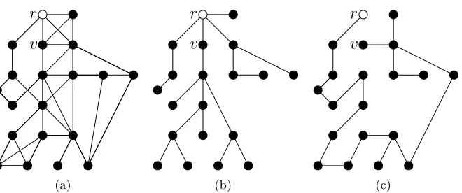
Figure 1: For a given graphGin Figure 1(a), Figure 1(b) contains a breadth-first spanning tree rooted atr extracted fromG, and Figure 1(c) contains a depth-first spanning tree rooted at r extracted from G.

is a cycle if the edge {vk, v0} is added to V(P). A graph that contains no

cycles as subgraphs isacyclic. A graph that has every unique pair of vertices

in some path in the graph is connected.

A tree is an acyclic, connected graph. Every tree with n vertices has

exactly n−1 edges. The vertices of a tree with a degree 1 are called its

leaves. Arooted tree is a tree where one vertex is designated as the root of

the graph. The depth of a vertex v in a tree rooted at r is the number of

edges in the path fromr tov. Theheight of a rooted tree is the number of

edges in the longest path from the root to some leaf vertex in the tree. A

vertexuin a rooted tree is theparent of vertexv if and only ifuis adjacent

to v and the depth of u in the tree is exactly one less than the depth of v.

If u is the parent of v, then v is a child of u and its siblings are the set of

all other children vertices of u. This relationship between a parent vertex

and its children is one-to-many: a vertex can only have one parent but it

can have many children.

Aspanning treeof a graphGis a tree where its vertices are exactly all the

vertices of Gand its edges are a subset of the edges ofG. Every connected

(9)

using traversal algorithms, such as depth-first or breadth-first search. The

breadth-first spanning tree in Figure 1(b) and the depth-first spanning tree

in Figure 1(c) illustrate how different traversal algorithms extract different

trees for the same graph shown in Figure 1(a). Breadth-first spanning trees

are particularly useful in graph theory and computer science because they

preserve the distance from the root vertex to any other vertex: the shortest

path distance from vertex v to the root r in Figure 1(b) is the same as it

is in the original graph in Figure 1(a), however, v’s shortest path distance

from v to r is much greater in Figure 1(c) than in Figure 1(a) and Figure

1(b).

A graph drawing represents pictorially the structure of a graph by placing

vertices at points on a plane and representing edges with curves between

these points [18]. More formally, a drawing Γ :V(G)∪E(G) → R2 ∪2R2

for a graphGis a function that maps each vertexv∈V(G) to a point Γ(v)

and each edge {u, v} ∈E(G), where u, v ∈ V (G), to a open Jordan curve

Γ({u, v}) with endpoints Γ(u) and Γ(v) [8].

Two graphs G = (V, E) and G0

= (V0_{, E}0

) are said to be isomorphic if

there exists a bijectionϕ:V →V0 _{such that for all} _{u, v} _∈_V_, _{_{u, v}_{} ∈}_E _⇔

{ϕ(u), ϕ(v)} ∈ E0_{. That is,} _G _and _G0 _{are isomorphic if they contain the}

same number of vertices connected by edges in the same way.

3 Graph Drawings

The art and science of graph drawing is matching problem domains with

algorithms and heuristics for producing visual representations of graphs.

In Section 3.1, we discuss three types of graph drawing parameters that

describe how a graph is drawn. In Section 3.2, we examine three examples of

(10)

and edges in a graph drawing.

3.1 Graph Drawing Parameters

Graph drawing parameters describe the visual characteristics of a graph

drawing. A graph drawing algorithm can use these parameters to produce

drawings that help users identify relevant attributes of a graph and facilitate

quick recognition of its important properties [8]. Graph drawing parameters

can accommodate the differences in spatial memory, reasoning abilities, and

visual predilections that users may have [63]. This may limit the scope of

a graph drawing system, and as such, many graph drawing parameters can

only be used for specific kinds of graphs or produce better results for graphs

of a certain type [8].

We now consider Battista, Eades, Tamassia, and Tollis’s division of graph

drawing parameters into three categories [8]: (1) general conventions for the

geometric representation of a graph (Section 3.1.1), (2) layout aesthetics

for producing a readable drawing (Section 3.1.2), and (3) constraints that

subgraphs in drawing may be required to satisfy (Section 3.1.3).

3.1.1 Drawing Conventions

Drawing conventions are application-dependant criteria that a graph

draw-ing must satisfy. When defined, conventions specify how vertices and edges

are represented in a graph drawing. Below we include a list of drawing

con-ventions from Battista et al. [8]. Figure 2 illustrates the differences of three

drawings of the same graph using different drawing conventions.

Straight Line: Edges must be drawn as a single line segment without any bends.

(11)

[image:11.612.137.473.124.228.2]

(a) Straight Line (b) Polyline (c) Grid Drawing

Figure 2: Three drawings of the same graph using different drawing conven-tions. The small circles at edge bends in Figure 2(b) and Figure 2(c) are added for emphasis.

Grid Drawing: Vertices must be positioned only at integer Cartesian co-ordinates on the drawing plane.

Planar Drawing: No two edges are allowed to intersect or overlap in the drawing.

Orthogonal Drawing: The graph must be drawn as a polyline grid draw-ing where the edges are only allowed to bend at right angles and are

comprised of alternating horizontal and vertical segments.

3.1.2 Aesthetics

Aesthetics are measurable properties used to evaluate the quality of a graph

drawing [6, 64]. Research suggests that if a drawing algorithm strongly

adheres to one or more carefully chosen aesthetic goals, it can create more

meaningful drawings [39, 58, 70]. Included below is Battista et al.’s list of

common graph drawing aesthetics [8]. When developing a graph drawing

algorithm, one seeks to optimize the presence of a particular aesthetic by

either minimizing or maximizing the measurable quality of the aesthetic.

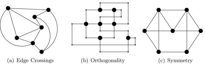
Figure 3 shows three drawings of the same graph that emphasize different

(12)

[image:12.612.129.464.123.228.2]

(a) Edge Crossings (b) Orthogonality (c) Symmetry

Figure 3: Three drawings of the same graph that adhere to different aes-thetic goals. The drawing in Figure 3(a) is constructed to minimize the number of edge crossings. The drawing in Figure 3(b) is constructed to maximize the orthogonal properties of the graph. The drawing in Figure 3(c) is constructed to maximize the symmetrical nature of the graph.

Planarity / Edge Crossings: The number of edge crossings in the draw-ing.

Area: The total area of a drawing.

Edge Length: Measuring the variance, the maximum length, or the sum total of edge lengths for all vertices or sets of vertices in a drawing.

Edge Bends: The number of separate line segments in a polyline edge.

Angular Resolution: Measuring the size of the angle between edges inci-dent to the same vertex.

Symmetry: Measuring the symmetrical properties of a graph drawing.

Orthogonality: Measuring the orthogonal nature of the graph drawing.

It is not always possible to optimize certain aesthetics within a graph

drawing. For instance, not every graph admits a planar drawing and when

no planar drawings exist it can be difficult to even find layouts that minimize

edge crossings. One might attempt to turn a graph into a planar graph by

(13)

a graph in order to make it planar. However, the problem of determining

for a given numberkand a graphGwhether it is possible to makeGplanar

by removing fewer thank of its edges is NP-hard [31].

Furthermore, as hard as it can be to optimize one aesthetic in a graph

drawing, it is often more difficult or impossible to simultaneously optimize

two or more [8]. A graph drawing algorithm must establish priorities for

the aesthetics that it uses because aesthetics may conflict. For instance,

although the drawings in Figure 3 depict the same graph, the drawing in

Figure 3(b) contains edge crossings but the drawing in Figure 3(a) does not.

It is a NP-hard problem in a straight-line graph drawing on an orthogonal

grid to minimize crossings while trying to minimize the total number of

edge bends [32]. An algorithm’s preference of one aesthetic over others will

influence the visual properties of the drawings it generates.

Purchase conducted studies on the effectiveness of various graph drawing

aesthetics [58]. Her experiments test which aesthetics best predicts a user’s

ability to answer questions about a graph. For each aesthetic, two graph

drawings were created; one having a strong presence of the aesthetic, and

the other a weak presence. Users were asked simple questions about each

drawing, such as what is the shortest path between two vertices. The

reac-tion times and error rates for the quesreac-tions determine how well a drawing

aesthetic improves a user’s ability to discern information from a graph.

Purchase concluded that the most significant factor for improving both

reaction times and error rates for graph drawings is minimizing the number

of edge crossings [58]. Additionally, minimizing the number of edge bends

substantially improved error rates and maximizing perceptual symmetry

slightly improved reaction times. Maximizing the orthogonal structure of

(14)

did not appear to have a significant effect on a user’s performance.

Ware, Purchase, Colpoys, and McGill extended Purchase’s work and

studied the impact of multiple aesthetics within a single graph drawing

instead of testing drawings representing the extremes of an aesthetics as

Purchase did [70]. Ware et al.’s also found that minimizing the number of

edge crossings in a graph drawing has the greatest positive impact on users.

A study by Huang and Eades used an eye tracking system to observe users’

eye movement patterns when viewing a graph drawing [39]. Like Ware et al.,

their results show that minimizing the number of crossings improves a user’s

ability to make judgments about a graph.

3.1.3 Drawing Constraints

Unlike drawing conventions and aesthetics, which are rules and criteria

ap-plied to the entire graph drawing, graphical drawing constraints are rules

that refer to specific subgraphs and subdrawings [8]. Constraints often

spec-ify the position of elements based on semantic information about the graph.

For instance, a constraint might specify that the most important vertex of

a graph is positioned at a particular location in the drawing. The list below

from Battista et al. contains commonly used constraints for drawing

algo-rithms [8]. Figure 4 shows three drawings of the same graph conforming to

different drawing constraints.

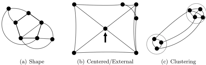
Centered Placement: Place a specific vertex at the center of the drawing.

External Placement: Place specific vertices at the outer areas of the drawing.

Clustered: Position vertex subsets close together.

(15)

[image:15.612.127.460.123.228.2]

(a) Shape (b) Centered/External (c) Clustering

Figure 4: Three drawings of the same graph using different graph drawing constraints. In the drawing in Figure 4(a), a subgraph forms the shape of a pentagon. In the drawing in Figure 4(b), a single vertex is placed at the center of the drawing (indicated by the arrow), while all other vertices are placed on the external edges of the drawing plane. The drawing in Figure 4(c) contains two subgraph clusters of vertices positioned together (indicated by the circle outlines).

Shape: Draw a subgraph in a pre-defined shape. Vertices can be positioned on the outline of the shape or edges can be drawn to conform to the

shape.

3.2 Drawing Algorithms

A drawing algorithm reads the description of a graph as its input, calculates

the positions of the graph’s elements on a viewing plane using graph drawing

parameters as guidelines, and outputs a drawing [8]. There are many

differ-ent classes of drawing algorithms [7]. We now examine a force-directed

lay-out algorithm that creates drawings using a physical system model (Section

3.2.1), a hyperbolic layout algorithm that creates fisheye-distorted drawings

(Section 3.2.2), and a radial layout algorithm that creates

(16)

3.2.1 Force-Directed Layout

A force-directed drawing algorithm creates graph drawings by simulating

repulsive and attractive forces [19]. Each vertex is assigned a repulsive force

and an initial position, and each edge is given an attractive force between

its endpoints. The resulting drawing represents a layout of the vertices and

edges in a locally minimal energy state. Eades’ original implementation of

the force-directed algorithm models vertices as electrically charged particles

that repel other vertices and edges as metal springs that pull adjacent

ver-tices toward one another [19]. Each spring’s pulling force becomes greater

as adjacent vertices repel each other, causing the spring to stretch. These

opposing forces cause non-adjacent vertices to move away from each other

while adjacent vertices are held close together. The simulation eventually

converges to an equilibrium state, where the pull at each vertex from the

springs is equivalent to the repulsion of the vertices. Other, more complex

force-directed models have been developed to use a more accurate

represen-tation of Hooke’s law for the behavior of springs [42], and reduce energy

factors through simulated annealing [16].

3.2.2 Hyperbolic Layout

Hyperbolic layout algorithms embed a graph’s elements in hyperbolic space

to produce drawings that have a distinct “fisheye” appearance. Like

Eu-clidean space, hyperbolic space consists of points, lines, planes and surfaces.

In hyperbolic space, however, there are many lines through a given point

which do not intersect a given line [15, 56]. A hyperbolic graph layout

algo-rithm creates a new drawing by first constructing a layout of the graph in

hyperbolic space, and then projecting this layout on to the Euclidean plane

(17)

[image:17.612.209.386.128.305.2]

r

Figure 5: A hyperbolic layout graph drawing for a tree rooted atr(adapted from [46]). In hyperbolic drawings, a graph’s elements are represented in space proportional to their distance to the root vertex; as vertices are posi-tioned further away from the root they become vanishingly small.

in space proportional to their distance from origin of the drawing; as an

ele-ment gets farther away from the origin, it is represented by smaller amounts

of space. An example of a hyperbolic layout graph drawing is shown in

Figure 5.

This distorted view of the graph is useful for viewing large hierarchies and

data sets [34]. Lamping, Rao, and Pirolli’s hyperbolic graph visualization

system generates two-dimensional drawings for subsections of the World

Wide Web [46]. Munzner expanded on their approach to project the graph

onto a three-dimensional viewing plane [50]. More recently, the Walrus

visualization tool by Hyun produces stunning hyperbolic visualizations for

trees with over a million vertices [40].

3.2.3 Radial Layout

Radial layout graph drawing algorithms are a well known method for

(18)

v

r

[image:18.612.134.462.125.298.2]

(a) (b)

Figure 6: A radial layout graph drawing of a tree rooted atr (Figure 6(a)) and the division levels ofv’s annulus wedge (Figure 6(b)).

6(a), the root vertex of a tree is positioned at the center of the drawing

with descendant vertices situated on concentric circles emanating from it.

For a tree T with a height k, the layers of concentric circles are labeled as

C1, C2, . . . , Ck and each vertex is placed on circle Ci, where i is the depth

of the vertex in the rooted tree [20, 59]. Using a defined heuristic, a radial

layout drawing algorithm allocates each vertex space in the drawing, known

as itsannulus wedge. This wedge confines the layout of a vertex’s subtree to

particular area in the drawing. A vertex’s annulus wedge is divided among

its descendants at subsequent levels in the subtree (Figure 6(b)).

For a tree T rooted at a vertexr, the radial positionsalgorithm (page

18) outputs a new radial layout graph drawing Γ forT. The algorithm first

places the root vertex at the center of the viewing plane and allocates it an

annulus wedge of the entire drawing (360◦

). This space is divided among

the root’s descendants: the annulus wedge for a child vertexc ofv is based

on the number of leaf vertices in the subtree rooted atcproportional to the

number of leaf vertices in the subtree rooted at v. Each vertex is placed at

(19)

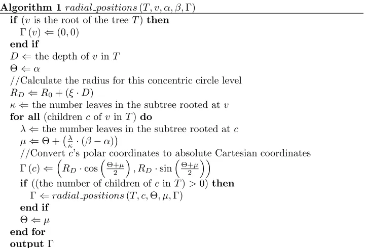
Algorithm 1radial positions(T, v, α, β,Γ)

if (v is the root of the treeT)then

Γ (v)⇐(0,0)

end if

D⇐the depth ofv in T

Θ⇐α

//Calculate the radius for this concentric circle level RD⇐R0+ (ξ·D)

κ⇐the number leaves in the subtree rooted atv

for all(childrencofv inT)do

λ⇐the number leaves in the subtree rooted atc

µ⇐Θ + λ

κ ·(β−α)

//Convertc’s polar coordinates to absolute Cartesian coordinates Γ (c)⇐RD·cos

Θ+µ

2

, RD·sin

Θ+µ

2

if ((the number of children ofcin T)>0)then

Γ⇐radial positions(T, c,Θ, µ,Γ)

end if

Θ⇐µ

[image:19.612.118.478.129.374.2]

end for outputΓ

Figure 7: Given a rooted treeT, a vertexv∈V (T), and the anglesα andβ

that definev’s annulus wedge, the algorithm calculates the position of every child vertex c ofv in a new graph drawing Γ. R0 is the user-defined radius

of the innermost concentric circle. ξ is the user-defined delta angle constant for the drawing’s concentric circles. The initial values for α and β for the root’s annulus wedge are 0◦

and 360◦

, respectively.

depth in the tree. The algorithm continues down each subtree until positions

for all of the graph’s vertices in the new drawing Γ are calculated.

Yee et al.’s Gnutellavision graph visualization tool uses theradial positions

algorithm to provide an overview of a peer-to-peer network [73]. In their

system, users select a host from the network to be the root of a

spanning-tree-based drawing. The concentric circles in their drawings represent the

network distance from the root to all other hosts; Each vertex is placed on

a circle corresponding to its shortest network distance to the root. A new

view of the network is constructed every time the user selects a new focal

point vertex.

(20)

[image:20.612.123.476.125.249.2]

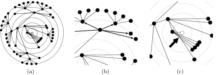
(a) (b) (c)

Figure 8: A radial layout graph drawing of the same tree from Figure 6, but with a different root vertex as the focal point. Figure 8(b) illustrates how sibling vertices have variable edge lengths to their parent, and Figure 8(c) highlights edge crossings in the drawing.

that help in creating sequences of drawings where a new drawing bears

some resemblance to the previous [73]. For example, their algorithm

man-dates that the direction of the edge between a newly selected root vertex

to its parent from the previous drawing is preserved. The new drawing also

preserves the rotational ordering of children vertices around their parent

from the previous drawing. Yee et al. believe that these features of their

system help users relate one drawing of a graph to the next.

However, like with any graph drawing algorithm, the drawings generated

by radial layout algorithms do have some drawbacks. Although the use of

concentric circles does make it easier for users to ascertain the depth of a

vertex in a tree, these circles confine vertices to positions that may not be

optimal and can make it difficult for users to visually distinguish siblings

from their parent. This is because sibling vertices may be spread out widely

on their corresponding circle, and thus the lengths of the edges to their

parent are dramatically different. For example, the drawings in Figure 8

depict the same tree from Figure 6 but based on a different root vertex. In

Figure 8(b), the edges marked by arrows illustrate edges for sibling vertices

(21)

can still allow edge crossings, even if the graph is planar (Figure 8(c)). As

the aesthetic usability studies have shown in Section 3.1.2, these flaws can

degrade the readability of a graph.

We now examine how graph animation aids in the visualization of graphs.

4 Graph Animation

In a graph animation, each frame in the animation sequence is a single graph

drawing that contains a subtle change from the previous drawing in the

sequence. When the frames are viewed in succession at an adequate speed,

the slight changes from one frame to the next is perceived as movement.

The entire animation sequence creates the illusion of the graph moving from

one layout to another.

Animation is an important feature in interactive graph visualization

sys-tems. Graph drawings in such system are susceptible to change by users and

outside stimuli, and users need to be informed of these changes in a way that

does not overwhelm them. Instead of instantaneously updating a drawing

for every change that occurs, a well-designed animated transition can

facili-tate visual continuity over multiple drawings of a graph [17, 29, 30]. Graph

animation should provide a smooth, continuous movement of a graph as a

means for revealing structural differences between two drawings while

pre-serving users’ mental maps [29]. A transition that is both visually appealing

and easy to follow helps users relate two separate graph drawings to one

an-other [21, 29].

Our discussion of graph animation used in visualization systems is as

follows. In Section 4.1, we discuss mental maps as they relate to graph

ani-mation. In Section 4.2, we discuss graph animation algorithms and present

(22)

4.1 Viewer Mental Map

Amental mapis a cognitive model of the spatial relationships between graph

elements that users form when viewing a graph [4, 22, 49, 65]. The concept

of a mental map is important to graph animation research because one seeks

to create a transition between multiple drawings of a graph that preserves

users’ mental maps. A good graph animation should not hinder users from

applying pre-existing knowledge about a graph to the new drawing. If it

is too difficult to relate a new drawing to the previous, users may have to

exert effort for each new drawing to regain familiarity with the graph [22].

Eades, Lai, Misue, and Sugiyama propose models for evaluating how well

two graph drawings resemble each other as an indicator for whether users

will be able to maintain mental map continuity when a visualization system

switches from one drawing to another [22]. For graph animation, Friedrich

and Eades propose models and metrics for how well an animation algorithm

transitions a graph, however, they do not conduct any experiments [29]. To

our knowledge, these metrics have not been used in human experiments.

4.2 Animation Algorithms

Given a graph and two drawings, which we call the initial and new layouts

of the graph, a graph animation algorithm generates a series of drawings,

called frames, of the graph that viewed sequentially, provides the illusion

of a smooth, continuous transition from the initial layout to the new

lay-out. As with graph drawing, animation algorithms are typically tailored to

emphasize the characteristics of the graph that are most important to the

intended audience [49].

One simple class of graph animation algorithms creates intermediate

(23)

ver-tices in the initial and new layouts [28, 38]. Although such algorithms may

work well on graphs with few elements, they are not practical for graphs

where hundreds of vertices may need to move great distances. This kind of

transition causes vertices to congregate together at particular locations in

the drawing, creating large swarms. These swarms reduce a user’s ability

to maintain his or her mental map of the graph; it is difficult to determine

which vertex came from which position when they are densely grouped

to-gether.

Alternative methods devised for generating animated graph transitions

seek to avoid the drawbacks found in the previous linear interpolation

exam-ple. We now describe three more sophisticated methods. First, in Section

4.2.1 we discuss an animation algorithm that creates rigid-body motion for

graphs. Next, we discuss a derivative work in Section 4.2.2 that generates

similar movements for individual subgraphs rather than a single movement

for the entire graph. Finally, in Section 4.2.3 we discuss an animation

algo-rithm for radial layout graph drawings.

4.2.1 Rigid-Body Animation

To alleviate vertex swarming problems that often occur in a transition

de-rived from a linear translation of Cartesian coordinates, Friedrich and Eades’

animation algorithm generates transition sequences that move a graph as a

solid object instead of as a collection of individual vertices moving

sepa-rately and erratically [29]. Such an approach is motivated by the belief that

the human brain is predisposed to follow uniform movements of objects [51].

The transition is divided into separate rigid motion and force-directed layout

stages. The graph first moves as a rigid object to position that is close to

(24)

algo-rithm then completes the transition using a force-directed simulation where

vertices are attracted to their destinations (instead of adjacent vertices).

Additionally, Friedrich and Eades use visual cues to help users anticipate

the animation better. When vertices or edges are to be removed from the

drawing during a transition, they gradually fade from view before the graph

begins to move. Likewise, when new vertices or edges are being added to the

drawing, they gradually fade into view only after the graph has reached its

final destination. Friedrich and Eades remark that the removal and addition

of graph elements before and after the transition reduces the amount of

visual distractions to users [29].

4.2.2 Clustered Movement Animation

Friedrich and Eades’ rigid-body animation is effective when a graph’s

ver-tices are uniformly distributed. The algorithm, however, performs poorly

for graphs that contain subgraphs whose optimal movement conflict with

the average optimal movement of the entire graph [30]. For example, even

if only a small part of a graph is altered, rigid-body animation algorithm

moves all vertices in the graph as a result. A derivative animation algorithm

by Friedrich and Houle adopts the same rigid-body-motion techniques from

Friedrich and Eades’ previous work, but apply it individually to subgraphs

[30]. Their algorithm uses clustering heuristics to identify subgraphs to share

uniform motion. The resulting animation sequences transition a graph as

separate components, each with its own unique movement. Users mentally

group subgraphs as separate objects and can follow the movements more

(25)

4.2.3 Radial Graph Animation

There are different animation methods for radial layout graph drawings

[41, 73]. Although many of the same animation criteria still apply, radial

layout transitions can have additional goals of maintaining vertex rotational

ordering and preserving the boundaries of subtrees.

Given a rooted treeT, a vertexv∈V (T), a time stepsin the animation

sequence, an initial drawing Γ1 of T and a new drawing Γ2 of T generated

by the graph drawing algorithm in Section 3.2.3, theradial transition

al-gorithm (page 25) computes the positions of v’s children at time step s

and outputs an intermediate drawing frame Γs. The algorithm calculates

the graph’s movement by interpolating the polar coordinates of vertices’

positions from Γ1 to Γ2. To generate all the intermediate frames for an

ani-mation, one would invoke this algorithm from time steps 1 toS, whereS is

the last frame in the animation sequence.

This animation algorithm creates two distinct types of motion for the

vertices of T. The root of the tree moves in a straight-line path from its

original position in Γ1 to the center of the new drawing. All other

non-root vertices move along radial paths to their new positions in Γ2. The

algorithm’s interpolation of vertices’ polar coordinates creates smooth

tran-sitions for radial graph drawings while avoiding occlusion problems that

can occur using a linear translation of Cartesian coordinates [73]. This

movement prevents vertices from amassing at the center of the drawing and

occluding one another.

Yee et al.’s Gnutellavision application uses the radial transition

algo-rithm to generate animated transitions when users select a vertex to become

the focal point of a new vertex-centric perspective of the Gnutella network

(26)

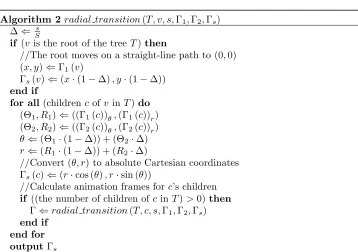
Algorithm 2radial transition(T, v, s,Γ1,Γ2,Γs)

∆⇐ s

S

//The root moves on a straight-line path to (0,0) (x, y)⇐Γ1(v)

Γs(v)⇐(x·(1−∆), y·(1−∆))

end if

(Θ1, R1)⇐((Γ1(c))_θ,(Γ1(c))_r)

(Θ2, R2)⇐((Γ2(c))_θ,(Γ2(c))_r)

θ⇐(Θ1·(1−∆)) + (Θ2·∆)

r⇐(R1·(1−∆)) + (R2·∆)

//Convert (θ, r) to absolute Cartesian coordinates Γs(c)⇐(r·cos (θ), r·sin (θ))

//Calculate animation frames forc’s children

Γ⇐radial transition(T, c, s,Γ1,Γ2,Γs)

[image:26.612.118.476.241.493.2]

end if end for outputΓs

Figure 9: Given a rooted treeT, a vertexv ∈V (T), the initial drawing Γ1for T, a new drawing Γ2 ofT, and the current time stepsin the animation, the

algorithm calculates the positions ofv’s children at time stepsand outputs an intermediate frame Γs. For any pointp~in a Cartesian coordinate system,

let (~pθ, ~pr) denote the polar coordinates of ~p. Let ∆ be the interpolation

(27)

algorithm’s interpolation factor (Section 6.2.3). Although only informal

hu-man experiments were conducted to validate this variable speed approach

in radial graph animations, Yee et al. claim users’ prefer exploring graphs

with this feature.

We now discuss user interactivity as it applies to graph visualization

systems.

5 User Interaction

Interactive visualization systems can often help users explore a graph more

easily than a single, static drawing. Herman, Melan¸con, and Marshall’s

survey of graph visualization discusses some of the more prevalent user

in-teraction techniques and facilities in graph visualization systems [34]. We

would now like to highlight three important concepts from their work.

5.1 Zooming and Panning

Herman et al. first discuss two user interaction capabilities found in many

visualization systems: zooming and panning. Visualization zooming can be

either geometric or semantic. Geometric zooming scales a visualization

sys-tem’s viewing plane to create either coarse overviews or detailed perspectives

of graphs. Semantic zooming alters the information content of a graph’s

el-ements according to some heuristic. Panning is simply a translation of the

viewing plane for a graph drawing.

5.2 Focus+Context

The focus+context graph visualization scheme creates drawings where an

area of interest in a graph is enlarged while other portions are shown with

(28)

focal point in greater detail and/or representing it with more geometric

space in the drawing [41]. Users interact with the visualization system by

changing the parameters that govern the focus+context distortion.

Herman et al. splits focus+context graph visualization implementations

into two categories: (1) the distortion is applied to a graph drawing after

it is generated, and (2) the distortion is integrated into the graph drawing

algorithm [34]. An example of applying the distortion after the drawing is

generated is the popular fisheye distortion technique [61, 62]. This approach

imitates a wide-angle lens to enlarge the area surrounding the focal point

in a display and shows peripheral areas of the graph with decreasing detail.

The drawback to this implementation, according to Herman et al., is that

because the distortion is applied after the drawing is generated, aesthetic

adherence may be degraded. Other visualization paradigms implement the

focus+context distortion directly in the graph drawing algorithm, such as

the hyperbolic layout algorithm in Section 3.2.2. This type of approach

allows systems to better control the effects of a focus+context distortion on

the drawing and mitigate the loss of aesthetic fulfillment.

5.3 Incremental Exploration

Inincremental exploration visualization systems, large graphs are displayed

in small portions instead overwhelming users with a single view of the entire

graph [34, 36, 38, 73]. These system create a “visible” window for a drawing

that allows users to explore subsections of the graph by moving the focus of

this window. Since the entire graph no longer needs to be known or

consid-ered all at once, incremental exploration systems are often more responsive

and computationally efficient.

(29)

37, 38, 53]. Eklund, Sawers, and Zeiliger’s NESTOR application creates

subgraph views of the World Wide Web; users are shown subsections of

the graph based on their web browsing histories [23]. Huang, Eades, and

Wang’s visualization system creates similar drawings but extend the visible

subgraph to include neighboring web pages that the user might visit [38].

6 Interactive Spanning Tree Visualization

Our graph visualization system allows users to explore the structure and

properties of a graph via multiple spanning-tree-based drawings. Given a

graph, the system first displays a force-directed layout of the entire graph,

using Eades’ simulation model of charged particles for vertices and metal

springs for edges [19]. A user then click on any vertex of the drawn graph.

A spanning tree rooted at the selected vertex is extracted from the graph

using breadth-first search. The system computes a drawing for the graph

based on this spanning tree, and then uses animation to transition from the

full graph drawing to this new drawing. Once this transition is complete,

users can select a new root vertex for a different layout or return to the full

graph view.

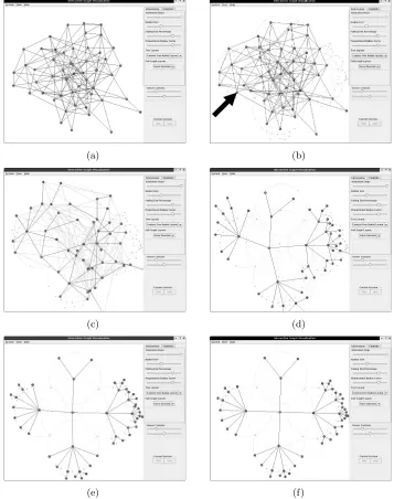
The screen captures in Figure 10 demonstrate how our visualization

sys-tem generates a force-directed layout drawing for the full graph, and then

transitions to a spanning tree drawing. The screen captures in Figure 11

demonstrate how our system generates a different spanning-tree-based

draw-ing rooted at a different vertex for the same graph in Figure 10, and then

transitions from the original drawing to the new drawing.

We now present our work on creating our graph visualization system in

two parts. First, in Section 6.1 we present our graph drawing algorithm,

(30)

we present our animation algorithm, which generates smooth, continuous

transitions between two graph drawings.

6.1 Context-Free Radial Layout

Given a graph G, a user-selected vertex r ∈ V (G), and an initial graph

drawing Γ for G, our graph drawing algorithm generates a new drawing of

G based on a spanning tree rooted at r extracted from G. We call our

algorithm “context free” because the placement of children, relative to the

frame of reference of the parent, only depends on the parent’s position.

We use this term loosely; drawing schemes that also have this property,

called shape grammars, have been studied more rigorously by other authors

[55, 57].

Our visualization system creates a new drawing for a graph G with an

initial drawing Γ in three stages. First it extracts a spanning treeTrooted at

r from G using breadth-first search. Using this tree, the system calculates

the graph’s vertices’ relative polar coordinates from their positions in Γ.

Based on these initial positions, the system then calculates the vertices’

relative polar coordinates in the new drawing. Instead of using concentric

circles where one circle is used for positioning all the vertices for a given

depth in the tree (Section 3.2.3), our algorithm creates drawings using a

series of overlapping circles that we call containment circles. Each

non-leaf vertexv ∈V (T) is given its own containment circle centered at v and

only v’s children are positioned on this circle. This approach enables the

drawing algorithm to position sibling vertices close together and emphasize

the parent-child relationships in the tree.

Before discussing the specifics of our new drawing method in Section

(31)

(a) (b)

(c) (d)

[image:31.612.118.475.138.590.2]

(e) (f)

(32)

(a) (b)

(c) (d)

[image:32.612.118.475.144.596.2]

(e) (f)

(33)

Algorithm 3initialLayoutAngleAndDelta(T, v,Υ1,Ω)

κ⇐The number of children ofv

//The root is allocated 360◦_{for its annulus wedge}

Ψ⇐ 360

κ

ϑ⇐the sum of all of the root’s children’s angles in Υ1

//Θ is the position of the root’s first child

Θ⇐ 1

κ·

ϑ−Ψ·κ·(κ+1) 2

else

//Calculate the bounding angles (α, β) forv’s annulus wedge of size Ω α⇐θ+ 360−1₂Ω

β⇐α+ Ω

//v’s annulus wedge is divided evenly between its children Ψ⇐ (β−α)

κ

//The initial angle Θ is the angle in the center of the first division Θ⇐α+1₂Ψ

end if

[image:33.612.118.476.278.500.2]

output(Θ,Ψ)

Figure 12: Given a rooted treeT, a vertexv∈V (T), and the initial drawing polar coordinate mapping Υ1, the algorithm outputs the angle position Θ

(34)

drawings.

6.1.1 Graph Drawing Parameters

Graph drawing parameters describe the visual characteristics of a graph

drawing (Section 3.1). The only convention our graph drawings follow is that

a graph’s edges are drawn as straight-line segments. The drawings adhere

to three aesthetic goals: (1) minimize the number of edge crossings, (2)

minimize the total angular difference between the root’s children’s positions

from the initial drawing to the new drawing, and (3) maximize the angular

resolution of parent-child edges. Our drawings conform to two constraints:

(1) the root vertex is placed at the center of the drawing, and (2) vertices

are equidistant to their parent vertex in the tree.

6.1.2 Layout Algorithm

Our context-free radial layout graph drawing algorithm computes a new

drawing for a spanning tree extracted from a graph. Instead of using

ab-solute Cartesian coordinates to position vertices, our algorithm computes a

mapping Υ :V (T) →(θ, r), where (θ, r) are polar coordinates for a vertex

v∈V (T) andT is a spanning tree extracted from a graphG. Our drawing

algorithm computes a mapping Υ1for the vertices’ coordinates in the initial

drawing Γ of a graph and a mapping Υ2 for the vertices’ coordinates in the

new drawing being generated. We use a polar coordinate system because

our animation algorithm computes animation sequences where vertices move

on radial paths by interpolating coordinates from Υ1 to Υ2 (Section 6.2.2).

One only needs Υ2 to convert the vertices’ polar coordinates to Cartesian

coordinates to generate the new static drawing of the graph.

(35)

Algorithm 4calculateP olarCoordsRelativeT oP arent(T, v, p, R,Ω,Γ,Υ1,Υ2) if (v is the root of the treeT)then

Υ1(v)⇐((Γ (v))_θ,(Γ (v))_r)

Υ2(v)⇐((Γ (v))_θ,0) end if

if ((the number of children ofv inT)>0) then

//Calculatev’s childrens’ polar coordinates relative tov’s position in Γ

Υ1(c)⇐((Γ (c)−Γ (v))_θ−(Υ1(v))_θ,(Γ (c)−Γ (v))_r) end for

//Calculate the initial angle Θ and the delta angle Ψ forv’s children (Θ,Ψ)⇐initialLayoutAngleAndDelta(T, v,Υ1,Ω)

if ((the number of children ofv inT) = 1)then

λ⇐ R

2 else

λ= 2R·sin Ψ₂

end if

//Calculatev’s childrens’ positions in the new drawing Υ2

for all(childrencofvinT, chosen according to the counterclockwise rotational ordering in Υ1of the children ofv)do

Υ2(c)⇐(Θ, R)

(Υ1,Υ2)⇐calculateP olarCoordsRelativeT oP arent(T, c, v, λ,Ω,Γ,Υ1,Υ2)

Θ⇐Θ + Ψ

end for end if

[image:35.612.117.478.216.535.2]

output(Υ1,Υ2)

Figure 13: Given a rooted tree T, a vertex v ∈ V (T), v’s parent vertex

p ∈ V (T), the radius R of v’s containment circle, and the initial graph drawing Γ, the algorithm calculates the relative radial coordinates of every child vertexc of v in the initial drawing mapping Υ1 and the new drawing

mapping Υ2. For any point ~p in a Cartesian coordinate system, let (~pθ, ~pr)

(36)

Algorithm 5initialLayoutAngleAndDelta(T, v,Υ1,Ω)

κ⇐The number of children ofv

//The root is allocated 360◦_{for its annulus wedge}

Ψ⇐ 360

κ

ϑ⇐the sum of all of the root’s children’s angles in Υ1

//Θ is the position of the root’s first child

Θ⇐ 1

κ·

ϑ−Ψ·κ·(κ+1) 2

else

//Calculate the bounding angles (α, β) forv’s annulus wedge of size Ω α⇐θ+ 360−1₂Ω

β⇐α+ Ω

//v’s annulus wedge is divided evenly between its children Ψ⇐ (β−α)

κ

//The initial angle Θ is the angle in the center of the first division Θ⇐α+1₂Ψ

end if

[image:36.612.118.476.279.500.2]

output(Θ,Ψ)

Figure 14: Given a rooted treeT, a vertexv∈V (T), and the initial drawing polar coordinate mapping Υ1, the algorithm outputs the angle position Θ

(37)

drawing Γ for T, the calculateP olarCoordsRelativeT oP arent algorithm

(page 34) computes the positions ofv’s children in the new drawing in four

parts: (1) if v is the root of T, position v at the center of the drawing,

(2) calculate v’s children’s relative polar coordinates in Υ1 based on the

children’s positions in Γ, (3) allocate a containment circle and an annulus

wedge to position v’s children in the new drawing, and (4) calculate v’s

children’s relative polar coordinates in Υ2 such that they are positioned

evenly onv’s containment circle within the bounds ofv’s annulus wedge.

First, the algorithm positions the root at the center of the new drawing

at (0,0). The root’s coordinates in Υ1 are derived by converting Γ (v) to

absolute polar coordinates. The root’s polar coordinate radius in Υ2 is set

at zero, but its polar coordinate angle is the same as in Υ1. This ensures

that the root moves on a straight-line path towards the origin of the drawing

during the animated transitions in our system (Section 6.2).

After the root’s coordinates are calculated in both Υ1 and Υ2, the

algo-rithm calculatesv’s children vertices’ polar coordinates in Υ1based on their

positions in Γ. For a child vertex c of v, c’s polar coordinate radius is the

Euclidean distance from Γ (c) to Γ (v) and its angle is relative tov’s position

in Γ.

Next, the system calculates the initial angle Θ for the first child of v,

and the delta angle Ψ separating v’s children on v’s containment circle in

the new drawing. For a tree T, a vertex v ∈ V (T), the initial drawing

mapping Υ1 forT, and the user-defined size of all non-root annulus wedges

Ω, theinitialLayoutAngleAndDeltaalgorithm (page 35) calculates relative

position of v’s annulus wedge and outputs the angle set (Θ,Ψ).

Ifv is the root of the tree,v’s annulus wedge is the entire angle space of

(38)

such that the angular difference from the root’s children’s positions in Υ1

to their positions in the new drawing is minimized. Although other layout

configurations may result in lower overall movement for the entire graph, our

algorithm only considers minimizing the rotational movement of the root’s

children.

Ifv is not the root of the tree,v’s annulus wedge is a portion ofv’s

con-tainment circle. The user-defined angle Ω specifies the size of v’s annulus

wedge, and the anglesα and β denote where on v’s containment circle the

wedge begins and ends. In order to adhere to our aesthetic goal of

maxi-mizing the angular resolution of parent-child edges, Ω is always less than or

equal to 180◦ _{(Ω is fixed at 180}◦ _{in the examples in Figure 15 and Figure}

16). The size of Ω influences the visual characteristics of the graph drawing:

smaller annulus wedges produce tighter and more narrow subtree layouts,

while larger wedges causes trees to fan out and use more space. The center

point ofv’s annulus wedge is the center of the arc onv’s containment circle

that is outside ofv’s parent’s circle. The size ofv’s annulus wedge is always

less than the size of this outer arc, and thusv’s children are not positioned

at overlapping circles’ intersection points (otherwise vertices would occlude

other vertices in neighboring circles). TheinitialLayoutAngleAndDelta

al-gorithm calculates the angles α and β using the angle from v to its parent

as the relative 0◦ _{in space on}_v_{’s containment circle.}

The vertexv’s annulus wedge is now divided into equal-sized portions for

each ofv’s children. Each child vertex is allocated the same amount of space

on v’s containment circle regardless of the size of its subtree. The initial

angle Θ is the center angle for the first subdivision of v’s annulus wedge.

The delta angle Ψ is the angular size of these annulus wedge subdivisions.

(39)

v’s entire annulus wedge.

Next, thecalculateP olarCoordsRelativeT oP arentalgorithm computes

the radius λof the containment circles for the next level of children in the

subtree. This radius λ is passed as the input for R in the next recursive

iteration of the drawing algorithm. If the number of children of v > 1,

then λ is the length of the chord from Θ to Θ +Ψ₂

on v’s containment

circle. If the number of children ofv= 1, thenλis R₂; this ensures that the containment circles in the drawing get progressively smaller as vertices are

positioned further away from the root.

The algorithm now iterates throughv’s children based on their

counter-clockwise rotational ordering in Υ1, and assigns each child a position in Υ2.

Like their coordinates in Υ1,v’s children’s positions in Υ2 are relative tov’s

position, but are now based onv’s new position in Υ2. For each child vertex

c of v, c’s polar coordinate radius in Υ2 is R, which is passed as input to

the algorithm, andc’s angle in Υ2 is Θ, which is incremented by Ψ for each

child. If v is the root of the tree, then the initial value for R is defined by

the user.

The drawing algorithm continues recursively down each subtree in a

depth-first fashion until all the vertices’ polar coordinates in Υ1 and Υ2 are

calculated. ThecalculateP olarCoordsRelativeT oP arentalgorithm runs in

O(n) time.

Figure 15 and Figure 16 provide a visual example of how our drawing

algorithm constructs a new spanning-tree-based drawing for a graph.

6.2 Animated Tree Transition

In our interactive graph visualization system, we provide animated

(40)

Ψ

Θ

R

r

(a)

v

r

(b)

α β

Ω

λ v

r

(c)

Θ

α+ Ψ

α v

r

[image:40.612.148.447.159.473.2]

(d)

Figure 15: The above diagram illustrates how our graph drawing algorithm constructs a new drawing for a treeT rooted atr. In Figure 15(a), the root is first placed at the center of the drawing along with its containment circle with a radius of R. The root’s annulus wedge is divided into three equal portions of size Ψ and its first child is positioned at Θ. In Figure 15(b), the root’s children are positioned on its containment circle. Next, in Figure 15(c) each of the root’s children is allocated a separate containment circle with a radius of λ. The algorithm then allocates space in the drawing to positionv’s children. v’s annulus wedge of size Ω is centered on the arc of

(41)

Ω

β

α

v

r

(a)

v

r

(b)

λ=R

2

R

(c)

v

r

(d)

[image:41.612.142.459.166.518.2]

(42)

present our graph animation algorithm that computes a sequence of frames

to transition any graph drawing to one of our spanning-tree-based drawings.

In Section 6.2.1, we first outline the particular goal we seek to

accom-plish with our graph animation algorithm. In Section 6.2.2, we discuss the

implementation specifics of our algorithm. In Section 6.2.3, we discuss two

auxiliary visual cues we incorporate into our system to further help users

maintain continuity during transitions.

6.2.1 Animation Goal

The principles of our animation algorithm are guided by previous graph

drawing aesthetic studies that suggest users are better able to comprehend

drawings that minimize the number of edge crossings [39, 58, 70]. Although

we are not aware of research that measures the effectiveness of drawing

aesthetics as applied to graph animation, we believe that the results of

these studies are certainly applicable to our work. Thus, the main goal in

our transitions from one drawing to another is to minimize the number of

crossings.

This goal is difficult to achieve because it is not a trivial task to

gen-erate an animation sequence for tree drawings with no edge crossings. For

example, the radial layout animation algorithm in Section 4.2.3 produces

crossings even when transitioning between two drawings of the same tree.

Rather than try to prevent all crossings, our animation algorithm is

de-signed to prevent two specific types: (1) crossings between sibling vertices,

and (2) crossings between the edge of a vertex to its parent with one of its

edges to its children. Our visualization system eliminates these crossings

because vertices’ positions are calculated relative to their parent and the

(43)

initial drawing.

In preventing these crossings, our algorithm does not calculate

move-ments simply by choosing the shortest path to move a vertex from one point

to another. We believe that the benefits of avoiding an edge crossing

out-weigh any increased movement in the animation.

6.2.2 Animation Algorithm

Our graph animation algorithm computes a series of frames that transition

a graph from an initial layout to a new drawing generated by our drawing

algorithm in Section 6.1.2. Given rooted tree T, a vertex v ∈ V (T), v’s

parent vertex p ∈ V (T), a time step s in the animation sequence, and

an initial drawing mapping Υ1 and a new drawing mapping Υ2 for T, the

transition algorithm (page 43) computes the positions of v’s children in

the animation sequence at time step s, and outputs a graph drawing frame

Γs. This frame is calculated by interpolating each vertex’s relative polar

coordinates from Υ1 to Υ2 using the parent’s position at the current time

step as a frame of reference. To generate all the intermediate frames for the

animation, one would invoke our algorithm from time steps 1 toS, where S

is the last frame in the animation sequence.

The algorithm first calculates the straight-line path movement of the root

vertex from its position in Υ1 to the center of the drawing at (0,0). The

difference between this straight-line movement and the radial movement of

all other vertices creates a visual contrast that allows users to easily identify

the new root of the tree.

Now the animation algorithm computes v’s children’s positions in Γs.

For a child vertex c of v, the algorithm first calculates c’s relative polar

(44)

in-Algorithm 6transition(T, v, p, s,Υ1,Υ2,Γs)

∆⇐ s

S

//The root moves on a straight-line path to (0,0) (θ, r)⇐Υ1(c)

(x, y)⇐((r·(1−∆))·cos (θ),(r·(1−∆))·sin (θ)) Γs(v)⇐(x, y)

ϕ⇐((0,0)−Γs(v))θ

else

(x, y)⇐Γs(v)

ϕ⇐(Γs(p)−Γs(v))_θ

end if

(Θ1, R1)⇐Υ1(c)

(Θ2, R2)⇐Υ2(c)

//Calculatec’s relative polar coordinates for this time-step θ⇐(Θ1·(1−∆)) + (Θ2·∆)

r⇐(R1·(1−∆)) + (R2·∆)

//Convert (θ, r) to absolute Cartesian coordinates for frame Γs

Γs(c)⇐(x+ (r·cos (θ+ϕ)), y+ (r·sin (θ+ϕ)))

//Calculate animation frames forv’s children

Γs=transition(T, c, v, s,Υ1,Υ2,Γs)

[image:44.612.117.476.210.523.2]

end if end for outputΓs

Figure 17: Given a rooted tree T, a vertex v ∈ V (T), v’s parent vertex

p∈V (T), the current time step sin the animation, and an initial drawing mapping Υ1 and a new drawing mapping Υ2, the algorithm calculates the

positions of v’s children at time steps and outputs an intermediate frame Γs. For any point~pin a Cartesian coordinate system, let (p~θ, ~pr) denote the

polar coordinates of~p. Let ∆ be the interpolation factor at time steps. Let

(45)

terpolation factor at time steps. These polar coordinates are then offset by

the reference angleϕandv’s position in Γs. If vis the root of the tree, then

ϕis the angle from Γs(v) to the center of the drawing at (0,0). Ifv is not

the root of the tree, thenϕ is the relative angle of v’s parent in Γs using v

as a point of reference. Ifchas children of its own, the algorithm recursively

invokes itself to calculate the positions for the vertices in the subtree rooted

at c.

The algorithm finishes once positions for all the vertices in the graph are

calculated for Γs. Thetransitionalgorithm runs inO(n) time.

Figure 18 and Figure 19 provide a step-by-step example of the how

ani-mation sequences are calculated by our aniani-mation algorithm.

6.2.3 Auxiliary Visual Enhancements

A graph drawing transition may visually overwhelm users with information

[29]. Although good graph animation alleviates many problems, additional

visualization techniques can further help users maintain their mental

conti-nuity between drawings. We now summarize the auxiliary visual

enhance-ments we use to improve the usefulness of the transitions created by our

animation algorithm.

First, we adopt the slow-in, slow-out timing used by Yee et al.’s

Gnutellav-ision system for the movements of vertices [73]. Variable speed approaches

such as this provide adequate visual constancy for users. This type of

move-ment mimics the acceleration and deceleration of massive objects in the real

physical world, which research suggests that the human brain is pre-disposed

to understand more easily [51]. To achieve this effect, our animation

algo-rithm calculates the interpolation factor ∆ from the curve of the arctangent

(46)

v

r

(a)

R2

R1

v

r

(b)

Θ1

Θ2

v

r

[image:46.612.132.436.167.492.2]

(c) (d)

Figure 18: The above diagram is an example of how our graph animation algorithm generates an animated transition for a treeT rooted atrto a new graph drawing. The algorithm first calculates the straight-line movement of the root, shown in Figure 18(a), from its initial position to the center of the drawing (denoted by the cross). The movement of vertex v is derived by interpolating from the radiiR1 to R2, shown in Figure 18(b), and from the

angles Θ1 to Θ2, shown in Figure 18(c). v’s movement is also based on its

(47)

(a)

r v

(b)

c1

c2

c4

c3

v

(c)

c3 c2

c1

c4

(d)

Figure 19: (Continued from Figure 18) The root’s children vertices move to their positions in the new drawing, shown in Figure 19(a) and Figure 19(b). The movements ofv’s children verticesc1,c2,c3, andc4’s are derived

[image:47.612.129.396.203.521.2]

(48)

in the animation and let S be the total number of steps in the animation

sequence:

∆⇐ 1

2

tan−1 s·10

S −5

tan−1₍₅₎

!

+1

2 (1)

Using this method of interpolation provides a “slow-start” movement

in the animation, allowing users to anticipate the general paths of vertices

in the ensuing transition. The movement of the graph accelerates to the

midpoint of the transition, and then decelerates as vertices reach their final

positions in the new drawing. With this timing, users are presented with a

transition that seems neither too fast nor too slow.

The second visual enhancement is the fading in and out of graph elements

used by Friedrich and Eades [29]. Our implementation differs from Friedrich

and Eades in that we fade elements during the transition, rather than before

and after. We believe that including transient edges during the animation

may allow users to study a graph more carefully; by having graph elements

gradually materialize and disappear as the graph moves, users also may be

able see the structural differences between two graph drawings with greater

ease.

The calculation of the fading factor during an animation sequence is

different for the two types of transition scenarios in our visualization system.

When transitioning from a spanning tree drawing back to the full graph, the

fading factor is based on a fixed delta for a finite time period. Because our

force-directed algorithm implementation is non-deterministic, we are unable

to fade relative to when the simulation will reach equilibrium.

The fading factor for spanning-tree-to-spanning-tree transitions in our

animation algorithm is relative to the current time step in the animation

Interactive, tree-based graph visualization

Rochester Institute of Technology

RIT Scholar Works

Theses

Thesis/Dissertation Collections

2006

Interactive, tree-based graph visualization

Andrew Pavlo

Follow this and additional works at:

http://scholarworks.rit.edu/theses

Recommended Citation

Interactive, Tree-Based Graph Visualization

Contents

1

Introduction

2

Graph Theory

3

Graph Drawings

v

r

4

Graph Animation

5

User Interaction

6

Interactive Spanning Tree Visualization